


1 Introduction
Hydrodynamic instabilities are ubiquitous to transport in porous media. Viscous fingering (VF) is one of these instabilities, which is observable while displacing a less-mobile fluid by another more-mobile fluid through porous media, and it plays critical roles in enhanced oil recovery through miscible flooding/solvent drive (Lake Reference Lake1989), chromatography separation (Guiochon et al. Reference Guiochon, Felinger, Shirazi and Katti2008), pattern formation (Li et al. Reference Li, Lowengrub, Fontana and Palffy-Muhoray2009), medicines (Bhaskar et al. Reference Bhaskar, Garik, Turner, Bradley, Bansil, Stanley and LaMont1992),  $\text{CO}_{2}$ sequestration (Moortgat Reference Moortgat2016; Amooie, Soltanian & Moortgat Reference Amooie, Soltanian and Moortgat2017; Li et al. Reference Li, Cai, Li, Li and Chen2019), diffusion-limited aggregation (Witten & Sander 1981), mixing (Jha, Cueto-Felgueroso & Juanes Reference Jha, Cueto-Felgueroso and Juanes2011) and bacterial colonies (Callan-Jones, Joanny & Prost Reference Callan-Jones, Joanny and Prost2008).
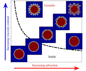
While advection is necessary for VF, diffusion stabilises this instability in miscible systems. For a given pressure gradient, the advection velocity is uniform in a rectilinear flow, whereas in a radial flow the velocity is inversely proportional to the radial distance from the point of fluid injection. The effects of diffusion on stabilisation of miscible fingering instabilities both in the linear and nonlinear regimes have been well understood mainly in the context of rectilinear displacement flows (Homsy Reference Homsy1987; Pramanik & Mishra Reference Pramanik and Mishra2015). In radial VF, the effects of diffusion at the initial stages of the displacement have been studied by Tan & Homsy (Reference Tan and Homsy1987), who concluded that the dispersion is strong enough to completely suppress the instability when the Péclet number  ${\sim}O(1)$; otherwise, the displacement is always unstable. On the other hand, Chui, de Anna & Juanes (Reference Chui, de Anna and Juanes2015) observed shut down of the overall flow instability emerging from the dominance of diffusion over advection at the later stages of the flow. More recently, the diffusion-driven transition between the two regimes of VF has been captured (Videbæk & Nagel Reference Videbæk and Nagel2019). Thus, there are many facets of the competition between advection and diffusion in radial flows. In contrast to this, Bischofberger, Ramachandran & Nagel (Reference Bischofberger, Ramachandran and Nagel2014) claimed that the viscosity ratio sets the velocity of the interface and three regimes of instability are obtained, for which the effects of diffusion are irrelevant. In this article, we show that the diffusion can never be neglected when dealing with miscible fluids. Initial stable displacement is the characteristic of dominant diffusion, which is equilibrated by advection at a later stage that is identified as the transition to an unstable state dominated by advection.
Further, we ask: can we control the competition between advection and diffusion to suppress the miscible radial VF? Diffusion, being an inherent property that depends on the displacing and displaced fluids, is difficult to tune; however, the advection can be suitably modified. Many studies focused on controlling VF (Dias et al. Reference Dias, Alvarez-Lacalle, Carvalho and Miranda2012; Zheng, Kim & Stone Reference Zheng, Kim and Stone2015; Yuan et al. Reference Yuan, Zhou, Wang, Zeng, Knorr and Imran2019) utilised time-dependent strategies to control advection. However, we achieve the same by merely modifying the initial configuration of radial displacement flow. We consider different initial finite volumes of the displacing fluid in the porous medium, which is represented by an initial radial distance ( $r_{0}$) of the interface from the centre of the porous medium. The effects of competition between advection and diffusion on the controllability of VF are parametrised in terms of
  $r_{0}$ and are explained through linear stability analysis (LSA) and compared with the corresponding nonlinear simulations (NLSs), supported by the result of a diligently designed experiment.
2 Mathematical model
The fluids considered are Newtonian, miscible, non-reactive with  $\unicode[STIX]{x1D707}_{l},\unicode[STIX]{x1D707}_{m}$ as viscosity of the less- and the more-viscous fluid, respectively. The non-dimensional governing equations for the flow in a two-dimensional (2-D) homogeneous porous medium are constituted by the Darcy’s law and the transport equation for the solute concentration
  $c$,
$c$,
 $$\begin{eqnarray}\displaystyle & \displaystyle \unicode[STIX]{x1D735}\boldsymbol{\cdot }\boldsymbol{u}=0, & \displaystyle\end{eqnarray}$$
 $$\begin{eqnarray}\displaystyle & \displaystyle \boldsymbol{u}=-\frac{1}{\unicode[STIX]{x1D707}(c)}\unicode[STIX]{x1D735}p,\quad \unicode[STIX]{x1D707}(c)=\text{e}^{(1-c)M}, & \displaystyle\end{eqnarray}$$
 $$\begin{eqnarray}\displaystyle & \displaystyle \unicode[STIX]{x2202}_{t}c+\boldsymbol{u}\boldsymbol{\cdot }\unicode[STIX]{x1D735}c=\frac{1}{Pe}\unicode[STIX]{x1D6FB}^{2}c, & \displaystyle\end{eqnarray}$$
 where  $p$ is the hydrodynamic pressure and
  $\boldsymbol{u}=(u,v)$ is the Darcy velocity vector. We use
  $t_{f}$, the total time of fluid injection, as the characteristic time, and
  $\sqrt{Qt_{f}}$ as characteristic length, where
  $Q$ is the gap-averaged flow rate. Consequently, we obtain two non-dimensional parameters: the Péclet number,
  $Pe=Q/D$, and the log-mobility ratio,
  $M=\ln (\unicode[STIX]{x1D707}_{m}/\unicode[STIX]{x1D707}_{l})$, where the molecular diffusion coefficient
  $D$ of
  $c$ in the solvent fluid is assumed to be a constant.

Figure 1. (a) Schematic of the computational domain  $\unicode[STIX]{x1D6FA}=[-L/2,L/2]\times [-L/2,L/2]$, with
  $L=3$ used for LSA and NLS. The centre of the domain is chosen as the origin of the cartesian coordinate system and the source of the less-viscous fluid initially occupying a circle of radius
  $r_{0}$. Here
  $M>0$. (b) Temporal evolution of
  $\ln (E(t))$ for
  $r_{0}=0.1$ to 0.3 with an increment 0.05. The onset time of instability is marked by ▫. The initial diffusion is prevalent for a longer time for a larger
  $r_{0}$ and, hence, the onset is delayed.
We consider a 2-D square domain  $\unicode[STIX]{x1D6FA}$ in the cartesian coordinates with the origin as the source of the less-viscous fluid (see figure 1a for computational domain). The initial condition associated with above equations is
  $\boldsymbol{u}(\boldsymbol{x},t=0)=\boldsymbol{x}/(2\unicode[STIX]{x03C0}|\boldsymbol{x}|^{2})$ and
 $$\begin{eqnarray}c(\boldsymbol{x},t=0)=\left\{\begin{array}{@{}ll@{}}1,\quad & 0\leqslant |\boldsymbol{x}|^{2}\leqslant r_{0}^{2}\\ 0,\quad & \text{otherwise},\end{array}\right.\end{eqnarray}$$
 where  $\boldsymbol{x}=(x,y)$, and
  $r_{0}$ is the non-dimensional radius of the initial circle occupied by less-viscous fluid.
3 Linear stability analysis
We perform LSA to identify the effects of diffusion at the initial stages of the displacement and the onset of VF. Assume the base state velocity is  $\boldsymbol{u}_{b}(\boldsymbol{x})=\boldsymbol{x}/(2\unicode[STIX]{x03C0}|\boldsymbol{x}|^{2})$, and the base state concentration
  $c_{b}$ is the solution of (2.3) for the initial condition (2.4). An analytical solution for this initial boundary value problem is not attainable. Following the analysis of Tan & Homsy (Reference Tan and Homsy1987) and Riaz, Pankiewitz & Meiburg (Reference Riaz, Pankiewitz and Meiburg2004), we search the base state concentration in terms of similarity variables, which is a powerful, well-established technique to solve partial differential equations (PDEs). However, similarity solutions to PDEs are almost always independent of any specific initial condition (Ball & Huppert Reference Ball and Huppert2019). Owing to this and the fact that the novelty of our work in this article is to find stability in miscible VF in terms of the initial condition of the displacement flow, a base state solution in terms of similarity variables is inappropriate. We use the method of lines to numerically compute
  $c_{b}$. Spatial derivatives are discretised using sixth-order compact finite differences (Lele Reference Lele1992) and the resulting initial value problem is solved using a third-order Runge–Kutta method. The velocity field is solved in the form of a stream function
  $\unicode[STIX]{x1D713}(x,y)$, defined as
  $u=\unicode[STIX]{x2202}_{y}\unicode[STIX]{x1D713}$,
  $v=-\unicode[STIX]{x2202}_{x}\unicode[STIX]{x1D713}$.
We introduce an infinitesimal perturbation ( $\unicode[STIX]{x1D713}^{\prime }$,
  $c^{\prime }$) such that
  $\unicode[STIX]{x1D713}=\unicode[STIX]{x1D713}_{b}+\unicode[STIX]{x1D713}^{\prime }$,
  $c=c_{b}+c^{\prime }$ (
 $\left|\unicode[STIX]{x1D713}^{\prime }\right|$,
  $\left|c^{\prime }\right|\ll 1$), where
  $\unicode[STIX]{x1D713}_{b}$ is the stream-function corresponding to
  $\boldsymbol{u}_{b}$. The corresponding linearised equations are solved for
  $\unicode[STIX]{x1D713}^{\prime }$,
  $c^{\prime }$ using the hybrid compact finite differences and the pseudo-spectral method. No flux boundary condition for
  $c^{\prime }$ and
  $\unicode[STIX]{x1D713}^{\prime }=0$ are used at the outflow boundary. The present LSA works as an alternative approach to study time-dependent linear system arising in miscible VF. Our interest does not lie in the wavelength selection like many other LSAs (Hota, Pramanik & Mishra Reference Hota, Pramanik and Mishra2015a), but in capturing initial diffusion and its effect on the onset of instability. However, it must be noted that our LSA is also applicable for wavelength selection (Hota, Pramanik & Mishra Reference Hota, Pramanik and Mishra2015b).

Figure 2. Natural logarithm of energy amplification as a function of time for (a)  $M=1$,
  $Pe=5000$, and (b)
  $M=3$,
  $Pe=1000$.
Recall that both  $c_{b}$ and
  $c^{\prime }$ evolve temporally. Therefore, the growth of
  $c^{\prime },\unicode[STIX]{x1D713}^{\prime }$ are relative to those of
  $c_{b},\unicode[STIX]{x1D713}_{b}$, and we quantify them at each instant of time. We define the energy ratio
 $$\begin{eqnarray}R(t)=E_{K}(c^{\prime },\boldsymbol{u}^{\prime })/E_{K}(c_{b},\boldsymbol{u}_{b}),\end{eqnarray}$$
 where  $E_{K}(c,\boldsymbol{u})=\int _{\unicode[STIX]{x1D6FA}}[c^{2}+\boldsymbol{u}^{2}]\,\text{d}\unicode[STIX]{x1D6FA}$ represents the kinetic energy at time
  $t$. The energy amplification,
 $$\begin{eqnarray}E(t)=R(t)/R(t=0),\end{eqnarray}$$
 is the ratio of the energy at time  $t$ to its value at
  $t=0$ (Matar & Troian Reference Matar and Troian1999). The nature of amplification as a function of time decides stability. An increasing or decreasing
  $E(t)$ indicates a relative growth or decay of the perturbations, while the presence of an extremum, if any, is of particular importance. A minimum indicates transition from a diffusion-dominating regime to an advection-dominated regime, which eventually implies the triggering of instability, whereas a maximum exhibits transient growths (Hota et al. Reference Hota, Pramanik and Mishra2015a). Figure 1(b) shows the natural logarithm of energy amplification as a function of time. Evidently,
  $\ln (E(t))$ is a non-monotonic function with a minimum occurring for each
  $r_{0}>0.1$. The minimum captures the competition between advection and diffusion in the linear regime. Up to the point of minimum, the disturbances are stabilised by the diffusive base state. The larger
  $r_{0}$, the later the point of minimum is obtained, indicating a delayed onset owing to the dominance of diffusive forces for a longer time. Similar qualitative results have been verified for various
  $M$ and
  $Pe$ as shown in figure 2. Therefore, our LSA captures controllability of VF owing to the competition between the two forces.
4 Nonlinear simulations

Figure 3. Density plots of concentration at  $t=1$ for
  $r_{0}=0.1$ and various
  $M$,
$M$,  $Pe$.
$Pe$.

Figure 4. (a) Temporal evolution of concentration contour  $c=0.5$ for
  $Pe=5000$,
  $M=1$ with
  $t=0$ (black), 0.5 (blue) and 1 (red). Increasing
  $r_{0}$ abates the instability as evident from the less-distorted contours at the same time for larger
  $r_{0}$. (b) Temporal evolution of normalised
  $I(t)$. Maiden deviation of the solid line (
 $M=1$) from the dashed line (
 $M=0$) marks the onset of instability.

Figure 5. (a) The  $M{-}Pe$ parameter space divided into stable and unstable regions for each
  $r_{0}$. The ordered pair
  $(Pe,M)$ below a curve corresponding to a given
  $r_{0}$ is associated with a stable displacement for the corresponding
  $r_{0}$. Inset: Plot of
  $\unicode[STIX]{x1D6FF}(t=1)$ versus
  $M$ for
  $r_{0}=0.1$. (b) Boundary between stable and unstable zones in the normalised
  $M_{c}$–
 $Pe_{c}$ parameter space.
To support the estimates of LSA that the instability is delayed as  $r_{0}$ increases, we perform NLS. We solve the coupled nonlinear equations (2.1)–(2.4) using a hybrid scheme based on compact finite differences and pseudo-spectral methods. This method has been used extensively to study instabilities in porous media (Chen et al. (Reference Chen, Huang, Wang and Miranda2010), Sharma et al. (Reference Sharma, Pramanik, Chen and Mishra2019), and references therein). We perform NLS for five different values of
  $r_{0}$, and for each
  $r_{0}$, we consider
  $M\in [0,3]$ and
  $Pe\in [500,10^{4}]$. A range of fingering dynamics from intense fingering to no instability at all are visible in the density plots of the concentration in figure 3 for
  $r_{0}=0.1$ on varying
  $M$,
$M$,  $Pe$. Similar results are also observed for other
  $r_{0}$. Further, we explore the effect of
  $r_{0}$ on the fingering dynamics. A comparison of the concentration contours at a given time for the two radii in figure 4(a) clearly depicts that fingering instability is abated as
  $r_{0}$ increases. Thus, the NLSs support the instability control predicted by LSA and indicate the existence of stable displacements despite an unfavourable viscosity contrast (i.e. when a less-viscous fluid displaces a more-viscous fluid) and high
  $Pe$.
$Pe$.
For each simulation, we compute the interfacial length (Mishra, Martin & De Wit Reference Mishra, Martin and De Wit2008),
 $$\begin{eqnarray}I(t)=\int _{\unicode[STIX]{x1D6FA}}|\unicode[STIX]{x1D735}c|\,\text{d}\unicode[STIX]{x1D6FA},\end{eqnarray}$$
 which measures the temporal variation of the concentration gradient. In figure 4(b), we plot  $I(t)$ normalised with its value at
  $t=0$, for
  $Pe=5000$. For
  $M=0$, we analytically calculate
  $I(t)=2\sqrt{\unicode[STIX]{x03C0}(t+\unicode[STIX]{x03C0}r_{0}^{2})}:=I_{0}(t)$ (say); in the absence of VF,
  $I(t)$ must coincide with
  $I_{0}(t)$. Further, we define
  $\unicode[STIX]{x1D6FF}(t)=|I(t)-I_{0}(t)|/I_{0}(t)$ and plot
  $\unicode[STIX]{x1D6FF}(t=1)$ versus
  $M$ for
  $r_{0}=0.1$,
  $Pe=3000,5000$ in the inset of figure 5(a). It is observed that
  $\unicode[STIX]{x1D6FF}(t=1)=0$ for
  $0\leqslant M\leqslant 0.75$ and
  $0\leqslant M\leqslant 0.575$, respectively, for
  $Pe=3000$ and 5000. This indicates
  $I(t)$ coincides with
  $I_{0}(t)$ even up to the final time for these parameters. Thus, for
  $M\in [0,0.75]$, the displacement is stable despite an unfavourable viscosity contrast for
  $Pe=3000$,
  $r_{0}=0.1$. Consequently, we use the value at the final time,
  $\unicode[STIX]{x1D6FF}(t=1)$, to classify the parameter set as stable or unstable. If
  $\unicode[STIX]{x1D6FF}(t=1)>0$, the corresponding parameter set (
 $r_{0}$,
  $M$,
$M$,  $Pe$) is identified as unstable; otherwise, it is identified as stable. Here
  $M=0.75$ and 0.575 lie on the boundary of the stable/unstable zone for
  $Pe=3000$ and
  $5000$, respectively, when
  $r_{0}=0.1$. Accordingly, for each
  $r_{0}$, we summarise the instability in the
  $Pe{-}M$ parameter space in figure 5(a). This indicates that for a fixed
  $M$, there is a critical Péclet number (or, similarly for a fixed
  $Pe$, there is a critical log-mobility ratio) for the occurrence of instability. The existence of a critical parameter for fingering instability in radial source flow with a point source (i.e.,
  $r_{0}=0$) has already been identified using LSA (Tan & Homsy Reference Tan and Homsy1987) and experiments (Bischofberger et al. Reference Bischofberger, Ramachandran and Nagel2014; Videbæk & Nagel Reference Videbæk and Nagel2019). Videbæk & Nagel (Reference Videbæk and Nagel2019) provide critical parameters that determine transition in the fingering patterns on account of diffusion. On the other hand, we are concerned with the transition between stability and instability, which arises due to competition between advection and diffusion. We would also like to emphasise that the initial condition in our study is different from that of Videbæk & Nagel (Reference Videbæk and Nagel2019).
Another quantification of the competition between advection and diffusion is sought in terms of  $I(t)$. An
  $I(t)$ identical to
  $I_{0}(t)$ indicates diffusion is the dominating force. We define
  $t=t_{on}$ as onset time of fingering in the nonlinear regime if
  $I(t)>I_{0}(t)$, for all
  $t$ satisfying
  $t_{on}\lesssim t<1$. Up to
  $t=t_{on}$, diffusion dominates advection and stabilises the displacement. For a larger
  $r_{0}$, the advection becomes weaker, consequently,
  $t_{on}$ is more for
  $r_{0}=0.15$, the larger radius shown in figure 4(b). Furthermore, from NLS we observe that
  $t_{on}$ increases with
  $r_{0}$ and the stable region spans over a larger range of both
  $M$ and
  $Pe$. It is noteworthy that the boundary between the stable and unstable regions follow a scaling relation
  $M_{c}=\unicode[STIX]{x1D6FC}(r_{0})Pe_{c}^{-\unicode[STIX]{x1D6FD}}$, with
  $0.52\lesssim \unicode[STIX]{x1D6FD}\lesssim 0.59$. We observe that for
  $\unicode[STIX]{x1D6FC}(r_{0})=30(1+10r_{0})$, the parameter pair (
 $M_{c},Pe_{c}$) lying on the boundary between the stable and the unstable regions can be well approximated by the relation
  $M_{c}=\unicode[STIX]{x1D6FC}(r_{0})Pe_{c}^{-0.55}$ (figure 5b). Therefore, using this scaling relation we can approximate the stability of radial flows in homogeneous porous media.
5 Experiments

Figure 6. Schematic of the experimental set up, showing the concentric pipes to inject the two fluids.
Our numerical results are further validated through state-of-the-art experiments. We used a radial Hele-Shaw cell with a gap width  $b=0.5~\text{mm}$. A hypodermic syringe needle (1.2 mm diameter and 40 mm length) bent in an L-shape and carefully embedded into a pipe was used to fill the two fluids in the Hele-Shaw cell. One may envision it as an annulus of L-shape pipe in straight outer pipe. The outer pipe is filled with more-viscous fluid while the inner pipe is filled with less-viscous fluid. This avoids the hassle of (a) changing the pipes for different fluids and (b) having a hole in each glass plate. A syringe pump (Cole-Parmer-D201253) was used for injecting the less-viscous fluid. Images were captured with a Sony FDR-AX40 camera. A schematic of the experimental set up is shown in figure 6. Aqueous glycerol (50 Vol.
  $\%$) solution with viscosity 6.8 mPa s was used as the less-viscous displacing fluid. The displaced more-viscous fluid was prepared with different percentage by volume of glycerol solution as listed in table 1. The viscosity of different aqueous glycerol solution was measured by a rheometer (Anton-Paar: MCR-702) and found to be in agreement with the calculated value through the mathematical formulation given by Cheng (Reference Cheng2008) and Volk & Kähler (Reference Volk and Kähler2018).
Table 1. Aqueous glycerol solution with different percentage by volume for making more-viscous fluid.

To obtain the initial circle of radius  $\bar{r}_{0}$, the less-viscous fluid was injected at a constant flow rate
  $Q_{1}~\unicode[STIX]{x03BC}\text{l}~\text{s}^{-1}$ for
  $t_{1}$ s in the Hele-Shaw cell, which was initially filled with the more-viscous fluid. The initial volume of the injected less-viscous fluid,
  $Q_{1}t_{1}~\text{ml}$, was chosen so that it leads to a stable displacement of the more-viscous fluid until the invading fluid occupies a circular region of radius
  $\bar{r}_{0}~\text{mm}$. Recall that during this stable displacement, the interface between the two fluids experiences diffusive spreading proportional to a length
  $\sqrt{Dt_{1}}$, which also contributes in
  $\bar{r}_{0}$; we measure
  $\bar{r}_{0}=\sqrt{Dt_{1}}+\sqrt{Q_{1}t_{1}/(\unicode[STIX]{x03C0}b)}$. Here,
  $D=10^{-9}~\text{m}^{2}~\text{s}^{-1}$ is the molecular diffusion coefficient of glycerol in water (D’Errico et al. Reference D’Errico, Ortona, Capuano and Vitagliano2004). We fixed
  $t_{1}=100$ s so that the amount of diffusion is the same for all the experiments and different
  $\bar{r}_{0}$ is obtained by varying
  $Q_{1}$ only. For example,
  $\bar{r}_{0}=15$, 18 and 20 mm were obtained by using
  $Q_{1}=3.3868$, 4.9121 and
  $6.086~\unicode[STIX]{x03BC}\text{l}~\text{s}^{-1}$, respectively.
As soon as the required dimensional radius  $\bar{r}_{0}$ was reached, the flow rate was increased to
  $Q^{\ast }$ and the less-viscous fluid was continuously injected at this flow up to a final time fixed for all the experiments. We repeated a series of experiments with
  $Q^{\ast }\in [0.05,0.5]~\text{ml}~\text{s}^{-1}$,
  $M\in [0,2.053]$, and capture suppression of the fingering instability for different values of
  $Q^{\ast }$ and
  $M$ qualitatively similar to NLS. No instability was observed for many
  $Q^{\ast }$ suggesting that there always exists a stable zone for each
  $\bar{r}_{0}$ as predicted by NLS for a range of
  $Pe$ and shown in figure 5. The experimental images at various time for
  $\bar{r}_{0}=18~\text{mm}$ and different
  $M$ and
  $Q^{\ast }$ are shown in figure 7. The effect of
  $Pe$ or
  $Q^{\ast }$ on the fingering dynamics is evident. For
  $Q^{\ast }=0.1~\text{ml}~\text{s}^{-1}$, the interface is slightly distorted near the final time, while
  $Q^{\ast }=0.5~\text{ml}~\text{s}^{-1}$ shows VF instability. In addition, increasing
  $M$ results in longer fingers and early onset as evident by comparing figures 7(a) and 7(b). The less-viscous fluid is dyed with Brilliant blue (BLENDS Ltd) food coloring dye to provide the visible contrast or optical observation to distinguish the two fluids. The amount of dye used is
  $0.01~\text{g}~\text{ml}^{-1}$ in the solution and has a negligible effect on viscosity.

Figure 7. Images from the experiments at different times for  $\bar{r}_{0}=18~\text{mm}$: (a)
  $M=2.053$,
  $Q^{\ast }=0.1~\text{ml}~\text{s}^{-1}$, (b)
  $M=2.053$,
  $Q^{\ast }=0.5~\text{ml}~\text{s}^{-1}$ and (c)
  $M=1.521$,
  $Q^{\ast }=0.5~\text{ml}~\text{s}^{-1}$. Pipes used for injecting the two fluids are also visible in the images. The black circle at the centre is the adhesive used for fixing the pipes to the Hele-Shaw cell.
The controlling effect of the initial radius  $r_{0}$ for
  $Q^{\ast }=0.4~\text{ml}~\text{s}^{-1}$ and
  $M=1.521$ is depicted in figure 8. We only show one quarter of the experimental images processed in MATLAB for better clarity. In addition, the validity of the control measure is justified on comparing with the experimental images for the point source (
 $r_{0}=0$) in figure 8(a). For visualisation purposes, we show the contours (plotted using the in-built command imcontour in MATLAB) of one quarter of the experimental images in figure 9(a). A delayed onset and reduced fingering corresponding to
  $\bar{r}_{0}=20~\text{mm}$ compared with
  $\bar{r}_{0}=15~\text{mm}$ for
  $Q^{\ast }=0.4~\text{ml}~\text{s}^{-1}$, and
  $M=1.521$ are evident. This supports the fact that the larger the
  $\bar{r}_{0}$, the weaker the advection and, hence, the initial competition between advection and diffusion determines the instability.

Figure 8. Experimental images at  $t=0$, 4800, 8000 and 9600 ms for
  $\bar{r}_{0}=$ (a) 0 (point source), (b) 15, (c) 18 and (d) 20 mm. Tip splitting and shielding are observable for
 $\bar{r}_{0}=0$ and are significantly absent for
  $\bar{r}_{0}\neq 0$. An abated instability with an increase in
  $\bar{r}_{0}$ is evident. A delay in instability is clearly visible on comparison of the snapshots for different
  $\bar{r}_{0}$. Here
  $Q^{\ast }=0.4~\text{ml}~\text{s}^{-1}$ and
  $M=1.521$.

Figure 9. (a) Contours at  $t=0$, 4000, 6000, 8000 and 9600 ms of the experimental images (shown in figures 8b and 8d for
  $\bar{r_{0}}=15~\text{mm}$ and
  $\bar{r_{0}}=20~\text{mm}$, respectively), showing the controlling effect of finiteness in terms of reduced and delayed instability. (b) Circularity as a function of time showing a delayed occurrence of distortions for larger
  $\bar{r}_{0}$.
We use ImageJ (Schneider, Rasband & Eliceiri Reference Schneider, Rasband and Eliceiri2012) to quantify the experimental results. To avoid the noise induced by the presence of the injection pipes in the images, we utilise half of the experimental domain in our analysis. For the validity of the control measure, the experiments should capture the initial radial displacement in the form of a circular displacing front. Circularity is used as a measure of the extent up to which the displacement front is circular (Escala et al. Reference Escala, De Wit, Carballido-Landeira and Muñuzuri2019). We define the circularity as
 $$\begin{eqnarray}C(t)=2\unicode[STIX]{x03C0}A(t)/P^{2}(t),\end{eqnarray}$$
 where  $A(t)$ and
  $P(t)$ correspond to the area and the perimeter of the region occupied by the less-viscous fluid, respectively, so that
  $C(t)=1$ for a semi-circle. For
  $P(t)$, we consider only the length of the curved surface since the diameter does not contribute to
  $C(t)$. Subject to experimental errors,
  $C(t)$ close to
  $1$ but constant over a range of time implies a circular displacing front. The maiden deviation of the circularity from the constant value indicates distortions at the front and it marks the triggering of the instability. Here
  $M=0$ works as the ideal radial source flow as no instability is observed as a result of equal viscosity of the two fluids. Hence,
  $C(t)$ for
  $M=0$ is used as the reference constant value for each
  $\bar{r}_{0}$. We found that
  $C(t)$ for
  $M\neq 0$ deviates from the constant value after some initial time for each
  $\bar{r}_{0}$ and the time of deviation is larger for larger
  $\bar{r}_{0}$ (see figure 9b for
  $Q^{\ast }=0.4~\text{ml}~\text{s}^{-1}$). In other words, the instability is triggered later for a larger
  $\bar{r}_{0}$. This confirms the qualitative agreement of the experiments with LSA and NLS. The proposed control measure can be used to control VF in a wide variety of radial source flows with miscible fluids.
6 Discussion and conclusion
Depending upon the application, controlling fingering instabilities is of paramount importance, for instance, instability can increase mixing while it is detrimental to oil recovery or separation processes. VF in immiscible systems are controllable by modifying the geometry (Bongrand & Tsai Reference Bongrand and Tsai2018; Pihler-Puzović et al. Reference Pihler-Puzović, Peng, Lister, Heil and Juel2018), using time-dependent strategies (Dias et al. Reference Dias, Alvarez-Lacalle, Carvalho and Miranda2012; Zheng et al. Reference Zheng, Kim and Stone2015), which may be directly inapplicable in miscible VF (Huang & Chen Reference Huang and Chen2015). In this article, we have investigated a stability mechanism in miscible VF by utilising the competition between the advective and diffusive forces.
Our theory takes care of the fact that the diffusive relaxation of the circular edge of the less-viscous inner fluid remains the same for all  $r_{0}$ considered. This has been implemented by choosing the initial condition (2.4), which clearly indicates that there is no initial diffusive relaxation present in the model. The dominance of diffusion over weaker advection for larger
  $r_{0}$ is responsible for stability. On the other hand, in experiments, we inject the less-viscous fluid for 100 s at different flow rate
  $Q_{1}~\unicode[STIX]{x03BC}\text{l}~\text{s}^{-1}$ to achieve different
  $\bar{r}_{0}$. In this way, the diffusive relaxation of the edges of the circular region happens the same for all different initial conditions. This ensures that diffusion-dominating advection due to the weakening of the latter for larger
  $\bar{r}_{0}$ causes stability. To understand the stability by analyzing the competition between advection and diffusion, we have used energy amplification in LSA, interfacial length in NLSs and circularity in the experiments.
Using LSA and NLS, we have obtained a criterion to control radial miscible VF and have shown that the radius of the initial circular region containing the displacing fluid is a control parameter. No modification in the geometry or a continuous variation in the flow rate is required unlike in many other earlier studies of immiscible VF (Dias et al. Reference Dias, Alvarez-Lacalle, Carvalho and Miranda2012; Zheng et al. Reference Zheng, Kim and Stone2015). Our theoretical results have been compared with experiments that are in qualitative agreement with the numerical results.
Time-dependent strategies, such as changing the flow rate in a rectilinear configuration (Yuan et al. Reference Yuan, Zhou, Wang, Zeng, Knorr and Imran2019) or varying the gap width of the Hele-Shaw cell in a radial configuration (Chen et al. Reference Chen, Huang, Wang and Miranda2010), have been attempted numerically in the context of miscible VF. Nevertheless, these studies lack sufficient evidence for the complete suppression of instability and have not validated experimentally. In contrast, we have successfully generated a stable radial experiment in accordance with our stability analysis and numerical simulations.
LSA predicts a delayed onset of instability with increasing  $r_{0}$, whereas NLSs predict a critical log-mobility ratio
  $M_{c}$ up to which there is no instability, dividing the
  $M{-}Pe$ plane into stable and unstable zones for each
  $r_{0}$. The log-mobility ratio and Péclet number on the boundary of the stable and unstable zones scale as
  $M_{c}=30(1+10r_{0})Pe_{c}^{-0.55}$. The stable zone increases with increasing
  $r_{0}$. Taking
  $r_{0}\rightarrow 0$ we approximate the critical
  $Pe$ for a point source radial flow, which, for a mobility ratio of 3, is
  ${\approx}65.8$, that is of the same order as estimated from linear stability by Tan & Homsy (Reference Tan and Homsy1987). For fixed values of
  $Pe$ and
  $M$, it is concluded that a stable displacement for a given
  $r_{0}$ ensures a stable displacement for all larger
  $r_{0}$ despite a favourable viscosity gradient. On the other hand, an unstable displacement for a given
  $r_{0}$ indicates a stronger and early instability for all smaller
  $r_{0}$ keeping
  $M$ and
  $Pe$ fixed. This corresponds to weakening of advection with an increase in the distance from the source. Experiments performed demonstrate the validity and the applicability of the proposed control strategy.
In addition to helping to understand the intrinsic properties of fundamental hydrodynamic instabilities (Paterson Reference Paterson1981; Tan & Homsy Reference Tan and Homsy1987; Bischofberger et al. Reference Bischofberger, Ramachandran and Nagel2014) and pattern formation (Witten & Sander 1981; Li et al. Reference Li, Lowengrub, Fontana and Palffy-Muhoray2009), our results suggest that the controllability of miscible VF in a radial configuration could be important in predicting the effectiveness of enhanced oil recovery by polymer flooding (Lake Reference Lake1989) and in various other similar configurations.
Acknowledgements
M.M. acknowledges the financial support from SERB, Government of India through project grant no. MTR/2017/000283. S.P. acknowledges the support of the Swedish Research Council grant no. 638-2013-9243. C.-Y.C. is thankful to ROC (Taiwan) Ministry of Science and Technology, for financial support through grant no. MOST 107-2221-E-009-070-MY3. V.S. acknowledges NCTU Taiwan Elite Internship Program for the financial support to visit C.-Y.C.
Declaration of interests
The authors report no conflict of interest.


