


1 Introduction
Historically, the macroscopic governing equations of fluid dynamics, i.e. the well-known Navier–Stokes equations, were derived from the basic principles of continuity of mass and momentum, with the assumption that the fluid at the macroscopic scale is a continuous substance (Batchelor Reference Batchelor2000). Note that the general form of the Navier–Stokes equations is essentially not closed, as the stress tensor is unknown except that a constitutive relation is assumed a priori. For Newtonian fluids, a reasonable assumption is that the stress tensor is linearly proportional to the local strain rate. For complex fluids or non-equilibrium flows, the constitutive relation is not so straightforward and usually depends on phenomenological models.
Although the Navier–Stokes equations have been widely applied to describe fluid flows, it is commonly believed that they fail in the description of flows at large Knudsen numbers ( $Kn>0.1$), where the non-equilibrium gas effect plays an important role (Bird Reference Bird1994). The Knudsen number is defined as the ratio between the molecular mean free path, i.e. the average distance travelled by one molecule between two subsequent collisions, and the characteristic chord length of the system, e.g. the chord length of an airfoil or the diameter of a cylinder. For non-equilibrium gas flows such as micro-flows and near-space flights, the Knudsen numbers are prone to be larger than 0.1, and thus a reliable set of equations above the Navier–Stokes level is highly desirable.
Theoretically, the macroscopic transport equations for non-equilibrium gas flows can be derived from the Boltzmann equation, which describes the microscopic behaviour of gases from a statistical point of view by accounting for molecular movements and collisions. One classical method for the derivation of macroscopic equations is the Chapman–Enskog method (Chapman & Cowling Reference Chapman and Cowling1990), which expands the distribution function around equilibrium state in a series of the Knudsen number. To the first order of Knudsen number, the Navier–Stokes equations are reproduced, while expansions to the second and third orders of Knudsen number give rise to the so-called Burnett and super-Burnett equations, respectively. Another method is Grad’s moment method (Struchtrup Reference Struchtrup2005), which expands the distribution function in Hermite polynomials, the coefficients of which are linear combinations of the moments. In Grad’s seminal work, he truncated the distribution function at the third order in Hermite polynomials and derived the well-known 13 moment equations (Struchtrup Reference Struchtrup2005). Afterwards, a lot of efforts have been made in this research direction, including the regularized 13 moment equations (Struchtrup & Torrilhon Reference Struchtrup and Torrilhon2003) and the regularized 26 moment equations (Gu & Emerson Reference Gu and Emerson2009; Gu et al. Reference Gu, Barber, John and Emerson2019). The applicability of these derived macroscopic governing equations to moderate non-equilibrium gas flows has been well validated, while the applicability to highly non-equilibrium gas flows is still limited and obscure.
Advances in machine learning (Jordan & Mitchell Reference Jordan and Mitchell2015; Duraisamy, Iaccarino & Xiao Reference Duraisamy, Iaccarino and Xiao2019; Brunton, Noack & Koumoutsakos Reference Brunton, Noack and Koumoutsakos2020) and data science (Marx Reference Marx2013; Brunton & Kutz Reference Brunton and Kutz2019) have provided engineers and scientists across all disciplines new opportunities for data-driven discovery, which has been referred to as the fourth paradigm of scientific discovery (Hey, Tansley & Tolle Reference Hey, Tansley and Tolle2009). Particularly, many concepts and methods from statistical learning can be employed to develop accurate models for complex dynamical systems directly from data. Methods for data-driven discovery of dynamical systems include equation-free modelling (Kevrekidis et al. Reference Kevrekidis, Gear, Hyman, Kevrekidid, Runborg and Theodoropoulos2003), artificial neural networks (Gonzalez, Rico & Kevrekidis Reference Gonzalez, Rico and Kevrekidis1998) and automated inference of the dynamics (Daniels & Nemenman Reference Daniels and Nemenman2015), just to name a few. In this series of developments, a seminal breakthrough was made by Bongard & Lipson (Reference Bongard and Lipson2007) and Schmidt & Lipson (Reference Schmidt and Lipson2009), who used symbolic regression to determine a nonlinear dynamic system from data directly. The disadvantage of symbolic regression is that it is usually expensive and prone to overfitting.
More recently, sparsity (Tibshirani Reference Tibshirani1996; Loiseau & Brunton Reference Loiseau and Brunton2018) has been used to determine, in a highly efficient computational manner, the governing equations of a dynamical system. Significant progress in this direction has been made by Brunton, Proctor & Kutz (Reference Brunton, Proctor and Kutz2016), who combined a sparsity-promoting technique and machine learning with nonlinear dynamical systems to discover ordinary differential equations (ODEs) from noisy measurement data. In particular, the sparse regression avoids overfitting by selecting parsimonious models that balance model accuracy with complexity. Only those terms that are most informative about the dynamics are selected as part of the discovered ODEs. Afterwards, Rudy et al. (Reference Rudy, Brunton, Proctor and Kutz2017) extended this method to handle spatio-temporal data or high-dimensional measurements and to discover the governing partial differential equations (PDEs) of the system. The algorithm they proposed is called PDE functional identification of nonlinear dynamics (PDE-FIND), which is computationally efficient, robust and has been successfully applied to a variety of canonical problems including fluid dynamics governed by Navier–Stokes equations. Note that a similar algorithm to PDE-FIND has also been proposed by Schaeffer (Reference Schaeffer2017) independently.
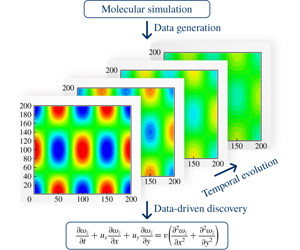
In the applications of PDE-FIND provided in the original work of Rudy et al. (Reference Rudy, Brunton, Proctor and Kutz2017), the data used to derive the PDEs were virtually generated by the numerical solutions of the associated governing equations. A more convincing demonstration would consider data from experimental observations or numerical simulations, which are independent of the derived governing equations. In this work, we generate spatio-temporal data of flow fields through a popular molecular simulation method, specifically, the direct simulation Monte Carlo (DSMC) method. DSMC method employs a large number of representative molecules to model gas flows. Note that, in the DSMC method, there is no need to assume any macroscopic governing equations a priori. The macroscopic quantities, such as density and velocity, are obtained by sampling molecular information and making an average at the computational cells. Theoretically, DSMC has been proved to be a particle method for solving the Boltzmann equation (Wagner Reference Wagner1992). Based on the spatio-temporal data obtained by DSMC, we derive the macroscopic governing equations for a variety of fluid flows using the PDE-FIND method.
Our ultimate objective is to develop general macroscopic governing equations for a wide range of non-equilibrium gas flows based on the data generated by DSMC, for which applicability to the whole range of Knudsen number flows has been validated. As a first step, in this work we focus on data-driven discovery of macroscopic governing equations at the Navier–Stokes level, i.e. in the continuum regime, where the theoretical macroscopic governing equations have been well established. The purpose is to verify that the data-driven discovery combined with molecular simulations is an alternative method to derive governing equations in fluid dynamics, besides the Chapman–Enskog expansion from the Boltzmann equation. To the best of our knowledge, this is the first time that macroscopic governing equations are derived by molecular simulations combined with a machine learning method.
The remainder of this paper is organized as follows. In § 2, we first describe the DSMC method for generating data, and then introduce the methodology for data-driven discovery, i.e. the PDE-FIND algorithm. In § 3, a variety of benchmark cases are provided to check the validity of our strategy for data-driven discovery of macroscopic governing equations, including the momentum equation, diffusion equation, Fokker–Planck equation and vorticity transport equation. Conclusions are given in § 4.
2 Methodology
2.1 DSMC method
The direct simulation Monte Carlo method was first proposed by Bird in the 1960s and is a stochastic particle-based algorithm to solve the Boltzmann equation by approximating the continuous molecular velocity distribution function with a discrete number of simulation molecules (Oran, Oh & Cybyk Reference Oran, Oh and Cybyk1998; Zhang et al. Reference Zhang, John, Pfeiffer, Fei and Wen2019a). Figure 1 is a schematic of the DSMC method, where each simulation molecule displayed by a blue sphere is randomly selected from a large number of real molecules. These simulation molecules are tracked as they move with their velocities, collide with other molecules and reflect from boundaries within a computational domain. Macroscopic gas properties are obtained by sampling corresponding molecular information and making an average at the computational cells, which are marked by red dashed lines in figure 1. Specifically, density ( $\unicode[STIX]{x1D70C}$) and macroscopic velocity (
 $u$) are given by,
 $$\begin{eqnarray}\displaystyle & \displaystyle \unicode[STIX]{x1D70C}=\frac{\displaystyle \mathop{\sum }_{i=1}^{N}m_{i}}{\unicode[STIX]{x1D6FF}V}, & \displaystyle\end{eqnarray}$$
 $$\begin{eqnarray}\displaystyle & \displaystyle u=\frac{\displaystyle \mathop{\sum }_{i=1}^{N}C_{i}}{N}, & \displaystyle\end{eqnarray}$$
 where  $m_{i}$ and
  $C_{i}$ are molecular mass and molecular velocity, respectively,
  $\unicode[STIX]{x1D6FF}V$ is the volume of the computational cell and
  $N$ is the number of molecules in the computational cell for sampling and averaging. To reduce statistical errors, a time average and ensemble average are usually used.

Figure 1. Schematic diagram of DSMC method.
For any application of the DSMC method, the first step is initializing simulation molecules according to the density distribution in the computational domain, and the following steps implement two sequential processes in each calculated time interval, i.e. molecular motions and inter-molecular collisions, which are assumed uncoupled during one time step. The molecular motions are implemented in a deterministic way, that is, every molecule moves ballistically from its original position to a new position, and the displacement is equal to the product of its velocity times the time step. If the predicted new position of one molecule crosses any boundary of the computational domain, an appropriate boundary condition needs to be applied. Specifically, the time at which the molecule hits the wall is first identified according to the distance between the molecule and the boundary divided by the molecular velocity, and then the molecular velocity reflected from the boundary is determined by the imposed gas–wall interaction model, such as specular, diffuse and Maxwell reflection models. Afterwards, the molecule moves according to its new reflected velocity within the remaining time of one calculating time step.
The inter-molecular collisions in the DSMC method are implemented in a probabilistic way, which is inherently different from other deterministic methods such as molecular dynamics. Several algorithms for the modelling of inter-molecular collisions have been proposed within the framework of DSMC. The most widely used model now is the no-time-counter (NTC) technique proposed by Bird (Reference Bird1994). In the NTC method, molecules in the same cells are randomly chosen as collision partners. The probability of selecting a collision pair is proportional to the relative speed between these two selected molecules. The post-collision velocities of molecules depend on the molecular model employed, which plays an important role for the accurate modelling of the real gas flows. The DSMC method allows for the introduction of phenomenological models such as the hard sphere (HS) and variable hard sphere models (Bird Reference Bird1994). For the argon gas at a fixed temperature used in this work, we employ the simplest HS model to describe interactions between gaseous molecules. Specifically, the molecular diameter is set to  $d=3.659\times 10^{-10}~\text{m}$, which is determined by the Chapman–Enskog theory and has been proven to give a correct prediction of viscosity.
The DSMC method was first applied to the simulation of high-speed gas flows in the context of aerospace engineering. Afterwards, the DSMC method has been successfully extended to investigate a variety of gas flows at the molecular level, such as micro-flows (Sun & Boyd Reference Sun and Boyd2002), flow instability (Stefanov, Roussinov & Cercignani Reference Stefanov, Roussinov and Cercignani2002; Zhang & Fan Reference Zhang and Fan2009; Zhang, Fan & Fei Reference Zhang, Fan and Fei2010; Manela & Zhang Reference Manela and Zhang2012) and even turbulence (Gallis et al. Reference Gallis, Bitter, Koehler, Torczynski, Plimpton and Papadakis2017; Zhang et al. Reference Zhang, Tian, Yao and Fei2019b). Theoretically, the DSMC method can be applied to simulate the whole regime of gas flows. It should be emphasized that, for an accurate simulation using the DSMC method, the time step needs to be smaller than the molecular mean collision time, and the cell sizes for the selection of collision pairs need to be smaller than the molecular mean free path (Alexander, Garcia & Alder Reference Alexander, Garcia and Alder1998; Garcia & Wagner Reference Garcia and Wagner2000).
2.2 PDE-FIND method
We employ the PDE-FIND algorithm proposed by Rudy et al. (Reference Rudy, Brunton, Proctor and Kutz2017) to derive the macroscopic governing equations based on the spatio-temporal results obtained by the DSMC method. Here, we just provide a brief description of the basic algorithm of the PDF-FIND method, and we refer readers to the original paper and supplementary materials (Rudy et al. Reference Rudy, Brunton, Proctor and Kutz2017) for details.
The spatial and temporal evolution of flow fields such as the velocity  $u(x,t)$ are obtained through DSMC calculations. We assume that the evolution of the flow field satisfies a PDE in terms of a general form as
 $$\begin{eqnarray}u_{t}=N(u,u_{x},u_{xx},\ldots )=\mathop{\sum }_{j=1}^{d}N_{j}(u,u_{x},u_{xx},\ldots )\unicode[STIX]{x1D709}_{j},\end{eqnarray}$$
 where  $N(\cdot )$ is a complex nonlinear function that can be expanded as a sum of simple monomial basis functions
  $N_{j}$ of
  $u$ and its derivatives multiplied by the corresponding coefficient
  $\unicode[STIX]{x1D709}_{j}$. The derivatives of the data with respect to time and space can be obtained using either a finite difference or polynomial interpolation method. Generally, the polynomial interpolation method performs better than the finite difference method if the data are associated with noise. Considering that the data generated from DSMC have inherent noise as DSMC is a stochastic particle method, the polynomial interpolation method is employed in this work to determine the derivatives.
Given a dataset comprising of  $m$ time steps and
  $n$ grid points, the data and their derivatives are constructed to form a linear problem as follows:

In (
2.4), each row represents an observation of the dynamics at a specific point in time and space, and  $\unicode[STIX]{x1D709}$ is a vector of coefficients which need to be determined. If we assume
  $\unicode[STIX]{x1D6E9}$ on the right-hand side of (
) is an over complete library, which has sufficient potential terms, then the dynamics of the system should be well described by the assumed governing equation. Theoretically, the candidate functions have arbitrary options including any order of nonlinearities and partial derivatives. Considering the characteristics of the fluid dynamics problems studied in this work, the highest-order term in  $\unicode[STIX]{x1D6E9}$ is composed of the third power of
  $u$ multiplied by the third derivative of
  $u$. For the sake of clarity, here, we list all the candidate functions considered for a one-dimensional problem, that is,
  $1,u,u^{2},u^{3},u_{x},uu_{x},u^{2}u_{x},u^{3}u_{x},u_{xx},uu_{xx},u^{2}u_{xx},u^{3}u_{xx},u_{xxx},uu_{xxx},u^{2}u_{xxx}$ and
  $u^{3}u_{xxx}$.
The key point in PDE-FIND is to select a sparse subset of active terms from the candidate functions, in other words, to determine the values of the vector of coefficients  $\unicode[STIX]{x1D709}$. If the coefficient of one specific term is non-zero, then the corresponding candidate function is selected. For an unbiased representation of the dynamics, one straightforward method for determining
  $\unicode[STIX]{x1D709}$ is to solve the least-squares problem. However, as reported by Rudy et al. (Reference Rudy, Brunton, Proctor and Kutz2017), the least-squares solution may be inaccurate even only with numerical round-off errors. In particular,
  $\unicode[STIX]{x1D709}$ tends to have non-negligible values, suggesting a PDE with all the prescribed functional forms in the library. In this way, the derived PDE is too complicated to be used, although it is mathematically correct. More importantly, the least-squares problem is essentially poorly conditioned for regression problems. Numerical error in computing the derivatives of the data could be magnified when inverting
  $\unicode[STIX]{x1D6E9}$. On the other hand, sparse regression has been demonstrated to be an efficient method, ensuring that the coefficients of the candidate functions which do not appear in the governing equations are exactly zero (Brunton et al. Reference Brunton, Proctor and Kutz2016). Recently, Rudy et al. (Reference Rudy, Brunton, Proctor and Kutz2017) proposed utilizing sparse regression to approximate the solution of
  $\unicode[STIX]{x1D709}$ as follows:
 $$\begin{eqnarray}\unicode[STIX]{x1D709}=\underset{\hat{\unicode[STIX]{x1D709}}}{\text{arg}\,\text{min}}\Vert \unicode[STIX]{x1D6E9}\hat{\unicode[STIX]{x1D709}}-\boldsymbol{U}_{t}\Vert _{2}^{2}+\unicode[STIX]{x1D706}\Vert \hat{\unicode[STIX]{x1D709}}\Vert _{0}.\end{eqnarray}$$
 This means that the prescribed terms only show up in the derived PDE if their effect on the error  $\Vert \unicode[STIX]{x1D6E9}\hat{\unicode[STIX]{x1D709}}-\boldsymbol{U}_{t}\Vert$ is greater than their addition to
  $\Vert \hat{\unicode[STIX]{x1D709}}\Vert _{0}$. The
  $\ell ^{0}$ term, i.e. the last term on the right-hand side of (2.5), makes this problem np-hard.
Specifically, the convex relaxation of the  $\ell ^{0}$ optimization problem in (2.5) can be written as
 $$\begin{eqnarray}\unicode[STIX]{x1D709}=\underset{\hat{\unicode[STIX]{x1D709}}}{\text{arg}\,\text{min}}\Vert \unicode[STIX]{x1D6E9}\hat{\unicode[STIX]{x1D709}}-\boldsymbol{U}_{t}\Vert _{2}^{2}+\unicode[STIX]{x1D706}\Vert \hat{\unicode[STIX]{x1D709}}\Vert _{1}.\end{eqnarray}$$
 This convex optimization problem can be solved by the least absolute shrinkage and selection operator (LASSO) (Tibshirani Reference Tibshirani1996). However, previous studies demonstrated that LASSO tends to have difficulty in finding a sparse basis if the columns in the matrix  $\unicode[STIX]{x1D6E9}$ are correlated. Recently, Rudy et al. (Reference Rudy, Brunton, Proctor and Kutz2017) proposed an alternative method, called the sequentially threshold least-squares (STLS) method. In STLS, a least-squares predictor is obtained and a hard threshold is performed on the regression coefficients. The process is repeated recursively on the remaining non-zero coefficients.
As reported by Rudy et al. (Reference Rudy, Brunton, Proctor and Kutz2017), STLS performed better than LASSO in most cases but still has the challenge of correlation in the data. In order to overcome this problem, ridge regression with an  $\ell ^{2}$ regularizer has been proposed by Rudy et al. (Reference Rudy, Brunton, Proctor and Kutz2017) to replace the least squares in STLS, that is,
 $$\begin{eqnarray}\hat{\unicode[STIX]{x1D709}}=\underset{\unicode[STIX]{x1D709}}{\text{arg}\,\text{min}}\Vert \unicode[STIX]{x1D6E9}\unicode[STIX]{x1D709}-\boldsymbol{U}_{t}\Vert _{2}^{2}+\unicode[STIX]{x1D706}\Vert \unicode[STIX]{x1D709}\Vert _{2}^{2}=(\unicode[STIX]{x1D6E9}^{\text{T}}\unicode[STIX]{x1D6E9}+\unicode[STIX]{x1D706}I)^{-1}\unicode[STIX]{x1D6E9}^{\text{T}}\boldsymbol{U}_{t}.\end{eqnarray}$$
This method is called sequential threshold ridge regression (STRidge) (Rudy et al. Reference Rudy, Brunton, Proctor and Kutz2017). A variation of test cases in the recent works Rudy et al. (Reference Rudy, Brunton, Proctor and Kutz2017, Reference Rudy, Alla, Brunton and Kutz2019) have demonstrated that STRidge has the best empirical performance. Note that a different threshold tolerance would result in a different level of sparsity in the final solution. To find the best tolerance, predictors are trained for varying tolerances and their performances are evaluated.
3 Results and discussion
3.1 Shear flow and momentum equation
We simulate two-dimensional unbounded flow of argon gas at standard conditions, i.e. pressure  $p=1.01\times 10^{5}\;\text{Pa}$ and temperature
  $T=273\;\text{K}$. According to the equation of state for perfect gases, the number density is
  $n=2.69\times 10^{25}~\text{m}^{-3}$. The computational domain is a square of side length
  $L=100\unicode[STIX]{x1D706}$, where
  $\unicode[STIX]{x1D706}$ is the molecular mean free path with the definition of
  $\unicode[STIX]{x1D706}=1/(\sqrt{2}\unicode[STIX]{x03C0}d^{2}n)$ for HS gas molecules. Consequently, the Knudsen number (
 $Kn=\unicode[STIX]{x1D706}/L$) is 0.01, and the flow can be considered to be in the continuum regime. Periodic boundary conditions are assumed in both directions. This means that, in the process of molecular movements, one molecule that gets through a specific boundary will re-enter the computational domain from the opposite boundary.
The whole computational domain is divided into  $256\times 256$ cells, and in each cell approximately 4000 simulation molecules are randomly distributed at the initial time, with one simulation molecule representing approximately
  $4\times 10^{6}$ real molecules. The initial thermal velocities of the simulation molecules are sampled randomly from a Maxwell distribution function at 273 K. The computational time step is set to
  $0.1\unicode[STIX]{x1D70F}$, where
  $\unicode[STIX]{x1D70F}$ is the molecular mean collision time with the definition of
  $\unicode[STIX]{x1D70F}=\unicode[STIX]{x1D706}/\overline{c}$. Note that
  $\overline{c}$ is the molecular mean speed, i.e.
  $\overline{c}=\sqrt{8kT/\unicode[STIX]{x03C0}m}$, where
  $k$ and
  $m$ are the Boltzmann constant and molecular mass, respectively. For the sake of clarity, the length scale and the time scale are normalized by the mean free path
  $\unicode[STIX]{x1D706}$ and the mean collision time
  $\unicode[STIX]{x1D70F}$, respectively. Correspondingly, the velocity and kinematic viscosity coefficient can be normalized by
  $\unicode[STIX]{x1D706}/\unicode[STIX]{x1D70F}$ and
  $\unicode[STIX]{x1D706}^{2}/\unicode[STIX]{x1D70F}$, respectively. In the following description, all the non-dimensional quantities are denoted with a superscript asterisk, for instance,
  $y^{\ast }$ represents the non-dimensional coordinate in the vertical direction.
To simulate a velocity decay process caused by viscous shear stress, we impose a spatially periodic macroscopic velocity field with a form of  $\boldsymbol{u}^{\ast }=u_{0}^{\ast }(1-\cos (2\unicode[STIX]{x03C0}y^{\ast }/L^{\ast }))\boldsymbol{e}_{\boldsymbol{x}}$ at the initial time, where
  $u_{0}^{\ast }=0.13$, and
  $\boldsymbol{e}_{\boldsymbol{x}}$ is the unit vector in the
  $x$ direction. For each simulation molecule, its initial velocity is a sum of two parts, i.e. the imposed macroscopic velocity and the random thermal velocity. In the simulation process, we obtain the macroscopic velocities for each cell by sampling of the molecular velocities in a short time period (10 mean collision times) and output the velocities on-the-fly, that is, at the time instants
  $t^{\ast }=0,10,20,\ldots ,1000$. Figure 2(a) shows the initial macroscopic velocity field generated in DSMC simulations. It can be seen from figure 2(a) that the flow is along the horizontal direction, and the amplitude of the horizontal velocity is uniform in the horizontal direction and only changes in the vertical direction. Note that fluctuations in the velocity field are caused by the molecular thermal motions, which are inevitable due to molecular thermal velocities in molecular simulations. To reduce the statistical fluctuations to an acceptable level, we make an average along the horizontal direction and focus on the changes in the vertical direction. Figure 2(b) shows the temporal evolution of the distribution of the horizontal velocity along the vertical direction. It can be seen that the initial distribution in terms of the cosine function gradually becomes smoother over time due to viscous dissipation.

Figure 2. (a) The velocity contours at the initial time obtained by DSMC simulations; (b) temporal evolution of the velocity distribution along the vertical direction.
We employ the values of the horizontal velocity at the discretized space–time points, i.e. 256 computational cells and 100 time instants, to construct the input dataset. Using the PDE-FIND method, we derive the governing equation in a parsimonious form, as shown in table 1. The coefficient of the term on the right-hand side is approximately 0.49 with a tolerance of  $\pm 0.01$. Note that, for the one-dimensional incompressible shear flow studied here, the non-dimensional Navier–Stokes equation can be simplified as follows:
 $$\begin{eqnarray}\frac{\unicode[STIX]{x2202}u^{\ast }}{\unicode[STIX]{x2202}t^{\ast }}=\unicode[STIX]{x1D708}^{\ast }\frac{\unicode[STIX]{x2202}^{2}u^{\ast }}{\unicode[STIX]{x2202}y^{\ast 2}},\end{eqnarray}$$
 where  $\unicode[STIX]{x1D708}^{\ast }$ is the non-dimensional viscosity coefficient. According to the Chapman–Enskog theory, the viscosity coefficient for a HS gas at the first-order approximation reads as (Chapman & Cowling Reference Chapman and Cowling1990)
 $$\begin{eqnarray}\unicode[STIX]{x1D708}=\frac{5\unicode[STIX]{x03C0}}{32}\unicode[STIX]{x1D706}\overline{c}=\frac{5\unicode[STIX]{x03C0}}{32}\frac{\unicode[STIX]{x1D706}^{2}}{\unicode[STIX]{x1D70F}}.\end{eqnarray}$$
 Therefore, the non-dimensional viscosity coefficient  $\unicode[STIX]{x1D708}^{\ast }$ is
  $5\unicode[STIX]{x03C0}/32\approx 0.49$. Comparing the derived governing equation with the theoretical counterpart in table 1, we can conclude that the derived governing equation not only has the expected form determined from the theoretical counterpart, but also gives an accurate estimation of the viscous coefficient.
Table 1. Governing equation for one-dimensional incompressible shear flow of argon gas.

It should be noted that the PDE-FIND method is sensitive to noisy data, and the data generated by molecular simulations inevitably have statistical fluctuations or errors. According to the theory of statistical mechanics, the fractional error of the velocity is inversely proportional to the square root of the sampling size (Hadjiconstantinou et al. Reference Hadjiconstantinou, Garcia, Bazant and He2003), that is,
 $$\begin{eqnarray}E_{u}\approx \frac{1}{\sqrt{N}Ma},\end{eqnarray}$$
 where  $N$ is the sampling size, and
  $Ma$ is the Mach number. Note that, in the preceding case of shear flow, there are approximately 4000 simulation molecules in each computational cell. To reduce fraction errors, we employ a short-time average (100 calculating time steps) and spatial average (256 computational cells in the horizontal direction) to obtain the temporal evolution of the velocity field in the vertical direction. Specifically, for each computational cell, the sampling size is
  $4000\times 100\times 256\approx 10^{8}$, and thus the fraction error at the initial time (
 $Ma\approx 0.3$) according to (3.3) is approximately
  $0.03\,\%$. As the simulation progresses, the macroscopic velocities and the Mach number decrease due to viscous dissipation, and hence the fraction error increases continuously. In this numerical case, the maximum fraction error of the viscosity coefficient in the derived equation is approximately
  $2\,\%$, as shown in table 1.
We run three other cases of the shear flow with different sampling sizes of  $10^{5}$,
  $10^{6}$ and
  $10^{7}$ for each computational cell, and the fractional errors of the velocity fields at the initial time are
  $1.0\,\%$,
  $0.3\,\%$ and
  $0.1\,\%$, respectively. If the initial fractional error is as large as
  $1.0\,\%$, we cannot obtain an expected governing equation. For the next two cases, the PDE-FIND method can derive governing equations in the right forms based on DSMC data, and the maximum fraction errors of the viscosity coefficient in the derived equations are
  $6.0\,\%$ and
  $4.0\,\%$, respectively. It is demonstrated that the accuracy of the derived governing equation using the PDE-FIND method is quite sensitive to noisy data. To obtain an expected derived equation, the fraction errors of the data generated by the molecular simulations must be reduced to an acceptable level.

Figure 3. (a) The density contours of species-A at the initial time obtained by DSMC simulations; (b) temporal evolution of density distribution of species-A along the vertical direction.
Table 2. Governing equation for the diffusion of argon gas.

3.2 Diffusion problem and diffusion equation
The simulation model for diffusion is also at the standard conditions, and it has the same geometry and boundary conditions as those employed for the shear flow in § 3.1. The differences are that two species of gas are employed to mimic the diffusion process, and the initial macroscopic velocity in the computational domain is set to zero uniformly. For the sake of simplicity, the two species are virtually like argon gas with the same molecular diameters, but are denoted as species-A and species-B. The initial distribution of non-dimensional densities for species-A and species-B are  $\unicode[STIX]{x1D70C}_{A}^{\ast }=0.5(1-\cos (2\unicode[STIX]{x03C0}y^{\ast }/L^{\ast }))$ and
  $\unicode[STIX]{x1D70C}_{B}^{\ast }=0.5(1+\cos (2\unicode[STIX]{x03C0}y^{\ast }/L^{\ast }))$, respectively. Figure 3(a) shows the density contours of species-A at the initial time. In the whole simulation process, the macroscopic velocity is always zero and the total density of the two species remains uniform in the computational domain, while the respective densities of species-A and species-B change with space and time. Therefore, the simulation model can be considered as a pure diffusion problem.
To reduce the statistical fluctuations, we also make an average of the density along the horizontal direction. Figure 3(b) shows the temporal evolution of the density distribution of species-A along the vertical direction. It is shown that the initial density distribution tends to be evenly distributed as the simulation proceeds due to the diffusion mechanism. Using the density of species-A at the discretized 256 computational cells and 100 time instants as the input dataset, we employ the PDE-FIND method to derive the corresponding governing equation, as shown in table 2. The coefficient of the term on the right-hand side is approximately 0.59 with a tolerance of  $\pm 0.01$. It is known that the non-dimensional diffusion equation with a constant diffusion coefficient is,
 $$\begin{eqnarray}\frac{\unicode[STIX]{x2202}\unicode[STIX]{x1D70C}^{\ast }}{\unicode[STIX]{x2202}t^{\ast }}=D^{\ast }\frac{\unicode[STIX]{x2202}^{2}\unicode[STIX]{x1D70C}^{\ast }}{\unicode[STIX]{x2202}y^{\ast 2}}.\end{eqnarray}$$
According to the Chapman–Enskog theory, the diffusion coefficient for a HS gas at the first-order approximation reads as (Chapman & Cowling Reference Chapman and Cowling1990)
 $$\begin{eqnarray}D=\frac{3\unicode[STIX]{x03C0}}{16}\unicode[STIX]{x1D706}\overline{c}=\frac{3\unicode[STIX]{x03C0}}{16}\frac{\unicode[STIX]{x1D706}^{2}}{\unicode[STIX]{x1D70F}}.\end{eqnarray}$$
 Therefore, the non-dimensional diffusion coefficient is  $3\unicode[STIX]{x03C0}/16\approx 0.59$. It can be concluded from the results shown in table 2 that the form of the derived governing equation for the diffusion problem agrees well with the theoretical diffusion equation, and gives an accurate estimation of the diffusion coefficient.
The advantage of molecular simulations like the DSMC method is that they not only can obtain the macroscopic quantities by sampling and averaging, but also provide molecular information such as the velocities and positions in detail. Our previous studies (Zhang et al. Reference Zhang, Fan and Fei2010; Zhang & Önskog Reference Zhang and Önskog2017; Zhang et al. Reference Zhang, Tian, Yao and Fei2019b) have demonstrated that on a time scale larger than the molecular mean collision time, the characteristics of molecular motion conform to Brownian motion. Therefore, it is intriguing to investigate whether the diffusion equation can be derived directly from molecular movements. To this end, in the simulation case of the diffusion problem, we randomly select 100 representatives from all the simulation molecules and record their positions every  $10\unicode[STIX]{x1D70F}$. Figure 4(a) shows one representative simulation molecule’s trajectory, that is, the position versus time, which seems like Brownian motion qualitatively.
In order to analyse the characteristics of molecular motions quantitatively, we first determine the molecular displacements  $\unicode[STIX]{x0394}y^{\ast }$ over any time interval
  $\unicode[STIX]{x0394}t^{\ast }$ based on 100 trajectories of selected simulation molecules, and then we obtain the probability density function of displacements by taking a statistical average for a specific time interval, i.e.
  $f(\unicode[STIX]{x0394}y^{\ast },\unicode[STIX]{x0394}t^{\ast })$, as shown in figure 4(b). It can be seen that the probability density functions conform to a normal distribution, and their variance increases with the time interval. These are virtually the typical characteristics of Brownian motion.

Figure 4. (a) A single trace of molecular motion; (b) probability density function of molecular displacements for different time intervals.
Using  $f(\unicode[STIX]{x0394}y^{\ast },\unicode[STIX]{x0394}t^{\ast })$ as the input dataset, we further employ the PDE-FIND method to derive the governing equation of the probability density function, as shown in table 3. Note that the mathematical symbol (delta) in front of
  $y^{\ast }$ and
  $t^{\ast }$ is dismissed for the sake of simplicity. According to the theory of stochastic processes, the Brownian motion can be described by the Wiener process using a Langevin-type equation, or equivalently, by a Fokker–Planck-type equation in terms of the probability density function. Specifically, the non-dimensional Fokker–Planck equation for Brownian motion with a constant diffusion coefficient and without any macroscopic velocities reads as,
 $$\begin{eqnarray}\frac{\unicode[STIX]{x2202}f}{\unicode[STIX]{x2202}t^{\ast }}=D^{\ast }\frac{\unicode[STIX]{x2202}^{2}f}{\unicode[STIX]{x2202}y^{\ast 2}},\end{eqnarray}$$
 where  $D^{\ast }$ is the non-dimensional diffusion coefficient, which has the same physical meaning as that in the diffusion equation and has the value of 0.59 for HS gas molecules. Comparing the two equations shown in table 3, we can conclude that the molecular motions in DSMC, over a time scale larger than the molecular collision time, can be described using a Fokker–Planck-type equation, with a well-defined diffusion coefficient based on kinetic theory.
Table 3. Governing equation for the molecular diffusion of argon gas.

3.3 Taylor–Green vortex and vorticity transport equation
The above two cases in §§ 3.1 and 3.2 are virtually one-dimensional as there are no gradients in the horizontal direction, and in the following we study one real two-dimensional problem of fluid dynamics. It is well known that, for two-dimensional incompressible viscous flow, the non-dimensional Navier–Stokes equations read as,
 $$\begin{eqnarray}\left.\begin{array}{@{}c@{}}\displaystyle \frac{\unicode[STIX]{x2202}u^{\ast }}{\unicode[STIX]{x2202}x^{\ast }}+\frac{\unicode[STIX]{x2202}v^{\ast }}{\unicode[STIX]{x2202}y^{\ast }}=0,\\ \displaystyle \frac{\unicode[STIX]{x2202}u^{\ast }}{\unicode[STIX]{x2202}t^{\ast }}+u^{\ast }\frac{\unicode[STIX]{x2202}u^{\ast }}{\unicode[STIX]{x2202}x^{\ast }}+v^{\ast }\frac{\unicode[STIX]{x2202}u^{\ast }}{\unicode[STIX]{x2202}y^{\ast }}=-\frac{\unicode[STIX]{x2202}p^{\ast }}{\unicode[STIX]{x2202}x^{\ast }}+\unicode[STIX]{x1D708}^{\ast }\left(\frac{\unicode[STIX]{x2202}^{2}u^{\ast }}{\unicode[STIX]{x2202}x^{\ast 2}}+\frac{\unicode[STIX]{x2202}^{2}u^{\ast }}{\unicode[STIX]{x2202}y^{\ast 2}}\right),\\ \displaystyle \frac{\unicode[STIX]{x2202}v^{\ast }}{\unicode[STIX]{x2202}t^{\ast }}+u^{\ast }\frac{\unicode[STIX]{x2202}v^{\ast }}{\unicode[STIX]{x2202}x^{\ast }}+v^{\ast }\frac{\unicode[STIX]{x2202}v^{\ast }}{\unicode[STIX]{x2202}y^{\ast }}=-\frac{\unicode[STIX]{x2202}p^{\ast }}{\unicode[STIX]{x2202}y^{\ast }}+\unicode[STIX]{x1D708}^{\ast }\left(\frac{\unicode[STIX]{x2202}^{2}v^{\ast }}{\unicode[STIX]{x2202}x^{\ast 2}}+\frac{\unicode[STIX]{x2202}^{2}v^{\ast }}{\unicode[STIX]{x2202}y^{\ast 2}}\right).\end{array}\right\}\end{eqnarray}$$
 Note that the length scale and the time scale are also normalized by the mean free path and the mean collision time, respectively;  $u^{\ast }$ and
  $v^{\ast }$ are the non-dimensional velocities in the horizontal and vertical directions, respectively. By defining the vorticity
  $\overrightarrow{\unicode[STIX]{x1D714}}=\unicode[STIX]{x1D735}\times \overrightarrow{v}$ and taking the curl of the Navier–Stokes equations, we can obtain the non-dimensional vorticity equation for two-dimensional incompressible flows as follows:
 $$\begin{eqnarray}\frac{\unicode[STIX]{x2202}\unicode[STIX]{x1D714}_{z}^{\ast }}{\unicode[STIX]{x2202}t^{\ast }}+u^{\ast }\frac{\unicode[STIX]{x2202}\unicode[STIX]{x1D714}_{z}^{\ast }}{\unicode[STIX]{x2202}x^{\ast }}+v^{\ast }\frac{\unicode[STIX]{x2202}\unicode[STIX]{x1D714}_{z}^{\ast }}{\unicode[STIX]{x2202}y^{\ast }}=\unicode[STIX]{x1D708}^{\ast }\left(\frac{\unicode[STIX]{x2202}^{2}\unicode[STIX]{x1D714}_{z}^{\ast }}{\unicode[STIX]{x2202}x^{\ast 2}}+\frac{\unicode[STIX]{x2202}^{2}\unicode[STIX]{x1D714}_{z}^{\ast }}{\unicode[STIX]{x2202}y^{\ast 2}}\right),\end{eqnarray}$$
 where  $\unicode[STIX]{x1D714}_{z}^{\ast }$ is the non-dimensional vorticity component in the
  $z$ direction, and
  $\unicode[STIX]{x1D714}_{x}^{\ast }=\unicode[STIX]{x1D714}_{y}^{\ast }=0$. In the community of fluid dynamics, the Taylor–Green vortex is widely used as a benchmark case in validating solvers and formulations in numerical computations, as it has an exact analytical solution to (3.7) and (3.8), that is,
 $$\begin{eqnarray}\left.\begin{array}{@{}l@{}}u^{\ast }=U_{0}^{\ast }\cos (2\unicode[STIX]{x03C0}x^{\ast }/L_{x}^{\ast })\sin (2\unicode[STIX]{x03C0}y^{\ast }/L_{y}^{\ast })\exp (-2v^{\ast }t^{\ast }),\\ v^{\ast }=-U_{0}^{\ast }\sin (2\unicode[STIX]{x03C0}x^{\ast }/L_{x}^{\ast })\cos (2\unicode[STIX]{x03C0}y^{\ast }/L_{y}^{\ast })\exp (-2v^{\ast }t^{\ast }).\end{array}\right\}\end{eqnarray}$$
 Here, we employ the DSMC method to simulate argon gas flow with initial conditions provided by the Taylor–Green vortex, and then we utilize the dataset obtained by DSMC to derive the underlying governing equation. Specifically, we simulate argon gas flow in a square of side length  $L_{x}^{\ast }=L_{y}^{\ast }=100$, and periodic boundary conditions are applied for all the boundaries. The initial macroscopic velocity is given by (3.9) at
  $t^{\ast }=0$, and we choose
  $U_{0}^{\ast }=0.08$ to ensure that the gas flow conforms to the assumption of incompressibility. The initial reference state is at standard conditions with uniform density and a small variation of pressure as
  $p^{\ast }=p_{0}^{\ast }-(\unicode[STIX]{x1D70C}_{0}^{\ast }U_{0}^{\ast 2})/4(\cos (4\unicode[STIX]{x03C0}x^{\ast }/L_{x}^{\ast })+\cos (4\unicode[STIX]{x03C0}y^{\ast }/L_{y}^{\ast }))$, to ensure that the initial conditions completely satisfy the solution of (3.7).
The whole computational domain is divided into  $64\times 64$ sampling cells, and each cell has approximately
  $4\times 10^{5}$ simulation molecules. The macroscopic quantities such as velocities are obtained by sampling the molecular velocities in the sampling cells. Each sampling cell is divided into enough sub-cells within which collision pairs are selected, and the sizes of the sub-cells are guaranteed to be less than the mean free path. We record the velocity field every 10 mean collision times (100 computational time steps) and obtain the vorticity field by taking the curl of the velocity vectors. To reduce the statistical errors, 10 independent runs with different random number sequences are performed to make an ensemble average. Figure 5 shows the contours of vorticity at
  $t^{\ast }=0,100,200,300$ obtained by DSMC. At the initial time (
 $Ma\approx 0.1$), the fraction error of the velocities according to (3.3) is approximately
  $0.05\,\%$. As shown in figure 5(a), our DSMC results are consistent with the theoretical results shown by the solid black lines, which are determined by (3.9). Due to viscous dissipation, the magnitude of the velocities and hence the Mach number would decrease as the simulation progresses. Consequently, the fractional errors increase continuously, as shown in figures 5(b), 5(c) and 5(d). Basically, our DSMC results agree well with theoretical results, and the maximum fraction error is less than
  $1\,\%$.

Figure 5. Contours of vorticity for the Taylor–Green vortex obtained by the DSMC method at different time instants: (a)  $t^{\ast }=0$; (b)
  $t^{\ast }=100$; (c)
  $t^{\ast }=200$; (d)
  $t^{\ast }=300$. The solid black lines represent the theoretical solutions of the Taylor–Green vortex.
Using the velocity and vorticity fields at  $64\times 64$ sampling cells and 65 time instants obtained by DSMC as the input dataset, we derive the governing equation shown in table 4. At first glance, the derived governing equation lacks two convective terms on the left-hand side compared with the theoretical vorticity transport equation shown in table 4. On the other hand, the two viscous terms on the right-hand side of the derived equation have the same forms as those in the theoretical equation, and their coefficients are quite close. Virtually, the derived governing equation is not wrong, but just in a simplified form for the specific problem of the Taylor–Green vortex.
It should be mentioned that the DSMC results are consistent with the exact analytical solution, equation (3.9), for the Taylor–Green vortex, except that the DSMC results are somewhat noisy. Substituting the velocity and vorticity fields determined by (3.9) into the two convective terms  $u^{\ast }(\unicode[STIX]{x2202}\unicode[STIX]{x1D714}_{z}^{\ast }/\unicode[STIX]{x2202}x^{\ast })$ and
  $v^{\ast }(\unicode[STIX]{x2202}\unicode[STIX]{x1D714}_{z}^{\ast }/\unicode[STIX]{x2202}y^{\ast })$, it is obvious that their sum is always zero. In this case, they are automatically eliminated in the derived governing equation, since the PDE-FIND method aims to find the most parsimonious form for the underlying governing equation.
In order to check whether the data generated by DSMC can derive the complete vorticity transport equation, we simulate another case with an artificial initial condition as follows:
 $$\begin{eqnarray}\left.\begin{array}{@{}l@{}}u^{\ast }=U_{0}^{\ast }\cos (4\unicode[STIX]{x03C0}x^{\ast }/L_{x}^{\ast })\sin (2\unicode[STIX]{x03C0}y^{\ast }/L_{y}^{\ast }),\\ v^{\ast }=-2U_{0}^{\ast }\sin (4\unicode[STIX]{x03C0}x^{\ast }/L_{x}^{\ast })\cos (2\unicode[STIX]{x03C0}y^{\ast }/L_{y}^{\ast }).\end{array}\right\}\end{eqnarray}$$
 Note that the wavenumber in the horizontal direction in (3.10) is double that of the standard Taylor–Green vortex. In order to satisfy the continuity equation of fluid dynamics, the amplitude of the velocity in the vertical direction is also doubled. The simulation domain is a square of side length  $L_{x}^{\ast }=L_{y}^{\ast }=200$, and other computation parameters are the same as those in the Taylor–Green vortex.
Figure 6 shows the contours of the vorticity field obtained by DSMC for the case with the artificial initial condition defined by (3.10) at  $t^{\ast }=0,100,200,300$. Using the dataset generated by DSMC, we also derive the governing equation, as shown in table 4. It has complete terms, including convective and viscous terms, as with the theoretical equation. The coefficients of the convective terms in the horizontal and vertical directions are 1.01 with a tolerance of
  $\pm 0.06$, while the coefficients of the viscous terms are 0.49 with a tolerance of
  $\pm 0.03$. The maximum relative error is approximately
  $6\,\%$ compared with the theoretical value. Considering that the DSMC results inevitably have noise as DSMC is a statistical simulation method, the prediction of the coefficients is acceptable. It is expected that we can get more accurate coefficients if we have larger sampling sizes, but this needs more computational resources.
Note that, in this work, we employ the simulation cases with an initial condition in terms of the Taylor–Green vortex and its variant to derive the vorticity transport equation. Essentially, the discovery of the vorticity transport equation is not limited to these special cases, and it can be realized as long as the flow problem is able to provide the spatial-temporal evolution of the velocity and vorticity fields, such as flow around a cylinder with shedding vortices.

Figure 6. Contours of vorticity fields for the case with artificial initial conditions obtained by the DSMC method at different time instants: (a)  $t^{\ast }=0$; (b)
  $t^{\ast }=100$; (c)
  $t^{\ast }=200$; (d)
  $t^{\ast }=300$.
Table 4. Governing equation for the diffusion of argon gas.

4 Conclusions
In this work, we employed the DSMC method on the molecular level to simulate three benchmark cases of fluid dynamics and obtained the data of the spatial-temporal evolution of the flow fields. The generated data are used to derive the macroscopic governing equations via the PDE-FIND method. Our simulation results of shear flow, diffusion problem and the Taylor–Green vortex obtained by DSMC are successfully applied to discover the momentum equation, diffusion equation and vorticity transport equation, respectively. For the diffusion problem, we also demonstrate that it is possible to derive the macroscopic equation using molecular information, such as the trajectories of the molecules instead of macroscopic quantities. The equations derived by the data-driven discovery method not only have the same form as the theoretical ones, but also provide accurate predictions of the transport coefficients contained in the governing equations.
This work provides strong proof that microscopic molecular movements and macroscopic flow phenomena governed by the underlying macroscopic equations have a close relationship, in terms of data-driven discovery. It should be noted that we have only focused on simple flow problems where the theoretical governing equations are well established so far, but the strategy proposed in this work can be extended to more complex problems such as rarefied gas flows, where the validity of the conventional Navier–Stokes equations is questionable and a variety of higher-order equation sets have been proposed. However, no single higher-order equation set has demonstrated universal superiority in the prediction of rarefied gas flows, especially for the capture of the Knudsen layer behaviour (Lockerby, Reese & Gallis Reference Lockerby, Reese and Gallis2005). Due to the complexity of the Knudsen layer and boundary conditions, the application of data-driven discovery of the governing equations to rarefied gas flows would be quite challenging. Research work in this direction is expected to be carried out in the future.
Acknowledgements
We thank S. L. Brunton and S. H. Rudy for providing the code of PDE-FIND method and stimulating discussions. This work was supported by the National Natural Science Foundation of China (grant no. 11772034). Results were obtained using the Tianhe-2 supercomputer.
Declaration of interests
The authors report no conflict of interest.


