2. Deflection due to a line load

As previously discussed, the simple linear two-dimensional model of Miles & Sneyd (Reference Miles and Sneyd2003) is further explored in this article. Thus the equations for the velocity potential $\phi (x,y,t)$ in the underlying water of density $\rho$ and depth $H$ and the deflection $\eta (x,t)$ of the floating thin elastic plate are

(2.1)$$\begin{gather} \frac{\partial^2 \phi}{\partial x^2}+\frac{\partial^2 \phi}{\partial y^2}=0 \quad (-\infty< x<\infty,-H< y<0), \end{gather}$$

(2.2)$$\begin{gather}D\frac{\partial^4 \eta}{\partial x^4}+\rho g \eta=\left.-\rho\frac{\partial \phi}{\partial t}\right|_{y=0}-p(x,t), \end{gather}$$

subject to

(2.3a,b)\begin{equation} \left.\frac{\partial \phi}{\partial y}\right|_{y={-}H}=0,\quad\left. \frac{\partial \phi}{\partial y}\right|_{y=0}=\frac{\partial \eta}{\partial t}, \end{equation}

where $D$ is the flexural rigidity of the plate and $p(x,t)$ is the pressure exerted by the load. The plate acceleration term is ignored (cf. Squire et al. Reference Squire, Hosking, Kerr and Langhorne1996). For a line load located at $x=X(t)$ such that $p(x,t)=p_0\delta (x-X(t))$, the one-dimensional form for the deflection obtained via Fourier–Laplace transforms may be rewritten as – cf. equation (2.13) in Miles & Sneyd (Reference Miles and Sneyd2003)

(2.4)\begin{equation} \eta(x,t) ={-}\frac{p_0}{2{\rm \pi} \rho} \int_{-\infty}^{\infty} {\rm e}^{{\rm i}kx}\frac{\tanh(kH)}{c(k)} \left(\int_0^{t} \exp({-{\rm i}kX(\tau)})\sin[kc(k)(t-\tau)]\,{\rm d}\tau\right)\,{\rm d}k, \end{equation}

where the appropriate positive branch of the phase speed

(2.5)\begin{equation} c(k) = \sqrt{\left(\frac{g}{k} + \frac{Dk^3}{\rho}\right)\tanh(kH)} \end{equation}

is symmetric in the wavenumber $k$. The time integral in (2.4) may be expressed as

(2.6)$$\begin{gather} \frac{1}{2{\rm i}} \int_0^t \exp({-{\rm i}kX(\tau)})\left(\exp({{\rm i}kc(t-\tau)}) - \exp({-{\rm i}kc(t-\tau)})\right)\,{\rm d}\tau=\frac{1}{2{\rm i}}\left[I(c) \exp({{\rm i}kct})\right.\nonumber\\ \left. -I({-}c)\exp({-{\rm i}kct})\right], \end{gather}$$

where

(2.7)\begin{equation} I(c)=\int_0^t \exp({-{\rm i}k\left[c\tau + X(\tau)\right]})\,{\rm d}\tau. \end{equation}

Thus adopting the real part of interest we have

(2.8)\begin{equation} \eta(x,t) ={-}\frac{p_0}{2{\rm \pi} \rho} \int_{0}^{\infty} \frac{\tanh(kH)}{c(k)} {\mathrm{Im}}\, \left[I(c)\exp({{\rm i}k(x+ct)})-I({-}c)\exp({{\rm i}k(x-ct)})\right]\,{\rm d}k, \end{equation}

involving the leftward propagating component

(2.9)\begin{equation} \eta_-(x,t)={-}\frac{p_0}{2{\rm \pi} \rho} \int_{0}^{\infty} \frac{\tanh(kH)}{c(k)} {\mathrm{Im}} \left[I(c)\exp({{\rm i}k(x+ct)})\right]\,{\rm d}k \end{equation}

and the rightward propagating component (in the direction of the load motion)

(2.10)\begin{equation} \eta_+(x,t)=\frac{p_0}{2{\rm \pi} \rho} \int_{0}^{\infty} \frac{\tanh(kH)}{c(k)} {\mathrm{Im}} \left[I({-}c)\exp({{\rm i}k(x-ct)})\right]\,{\rm d}k. \end{equation}

3. Impulsively started steadily moving loads

In this section, we consider the evolution of responses to steadily moving line loads that are impulsively started, when implicitly no account is taken of prior loading (cf. Squire et al. Reference Squire, Hosking, Kerr and Langhorne1996; Miles & Sneyd Reference Miles and Sneyd2003). Thus the deflection $\eta (x,t)$ is calculated for loads that are switched on impulsively at time $t=0$ and then move steadily, such that $X(t)=Vt,\,t>0$ where $V$ is constant. We adopt Takizawa data similar to Miles & Sneyd (Reference Miles and Sneyd2003) – viz. Young's modulus $E = 1.79 \times 10^8$ Pa, plate thickness $h=0.14$ m, Poisson ratio $\nu =1/3$, water density $\rho =1026$ kg m$^{-3}$ and water depth $H=6.80$ m. The critical speed $c_{min}$ is a little over 5 m s$^{-1}$, and the gravity wave speed is $\sqrt {gH}=8.16$ m s$^{-1}$. The deflections illustrated in this section are in the frame of motion of the load.

All of the results reported in this article were obtained by analytically evaluating the integral in $t$ that appears in (2.4), and then approximating the inverse Fourier transform by a discrete inverse Fourier transform that produces a set of linear equations relating the deflection at a discrete set of spatial values to the Fourier transform of the deflection at a discrete set of wavenumber values. The fast Fourier transform was employed to solve this system of equations to obtain the deflection. In the case of impulsively started loads, the application of the discrete inverse Fourier transform is justified since the integrand in (2.4) has no poles on the real axis. When the initial condition corresponding to a steadily moving load is introduced, the modified integrand corresponding to (2.4) has poles on the real axis for values of $k$ where $V^2-c^2=0$. The part of the integrand corresponding to the initial conditions must then be modified, so that the contribution from the poles can be calculated analytically and the discrete inverse Fourier transform can be applied to approximate what remains. Appendix A provides further details.

We first present mesh plots that show the evolution of the deflection in the $(x,t)$-plane, which directly compare figures in Miles & Sneyd (Reference Miles and Sneyd2003) for two illustrative load speeds. The $x$-axis in metres is again placed in the immediate foreground in figures 2 and 3, but on the second horizontal axis we prefer to represent the equivalent time span in seconds. For an impulsively started load that then moves at the subcritical speed $V=2$ m s$^{-1}$, we found the deflection starts to reflect the familiar quasi-static form due to the corresponding steadily moving load, as shown in figure 2, which resembles figure 1(a) of Miles & Sneyd (Reference Miles and Sneyd2003). 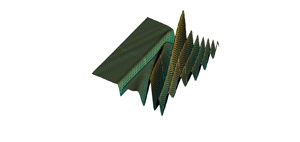The deflection we obtained for an impulsively started load that then moves at constant supercritical speed $V=1.17 c_{min}$ shown in figure 3 also resembles figure 1(b) of Miles & Sneyd (Reference Miles and Sneyd2003), where characteristic leading predominantly flexural waves and trailing predominantly gravity waves appear. The longer time taken for the trailing waves to more clearly emerge is shown in figure 4. The response for a higher impulsively started constant supercritical speed $V=10$ m s$^{-1} > \sqrt {gH}$ at $t = 8$ s in figure 5 shows that the leading predominantly flexural wave is then accompanied by a trailing transient, which dissipates as the shadow zone emerges, as seen in figure 6. While each of the three different steady-state forms quickly emerge near the load, the emergence of the steady-state takes longer elsewhere – but we recognise the restricted propagation to the line of motion in the two-dimensional model is an extenuating factor. (The present context is accordingly called one-dimensional in Wang et al. (Reference Wang, Hosking and Milinazzo2004), where ‘one-dimensional’ and ‘two-dimensional’ refer to the flexural-gravity wave propagation in the floating ice plate, but in this paper we have used the now more common terminology acknowledging the additional vertical dimension.)

Figure 2. The evolution of the deflection due to an impulsively started steadily moving load at the subcritical speed $V=2$ m s$^{-1}$ over the first 8 s for the Takizawa data, in a direct comparison with figure 1(a) of Miles & Sneyd (Reference Miles and Sneyd2003). The familiar constant load speed quasi-static form shown in red begins to emerge as the transients propagate away.

Figure 3. The evolution of the deflection due to an impulsively started steadily moving load at the supercritical speed $V=1.17 c_{min}$ m s$^{-1}$ over the first 16 s for the Takizawa data, in a direct comparison with figure 1(b) of Miles & Sneyd (Reference Miles and Sneyd2003). The familiar constant load speed wave form shown in red begins to emerge as the transients propagate away.

Figure 4. The evolution of the deflection at the impulsively started supercritical load speed $V=1.17 c_{min}$ m s$^{-1}$ for the Takizawa data, showing the time taken for the longer trailing predominantly gravity wave to more clearly develop.

Figure 5. The deflection for the impulsively started higher supercritical load speed $V=10$ m s$^{-1}$ $>\sqrt {gH}$ at 8 s for the Takizawa data. The short wavelength leading predominantly flexural wave is followed by trailing transients propagating away from the load.

Figure 6. The deflection for the impulsively started supercritical load speed $V=10$ m s$^{-1}$ $>\sqrt {gH}$ at 25, 50 and 100 s for the Takizawa data. The transients behind the load propagate away rather slowly as the shadow zone develops.

Incidentally, to render the deflections in metres at any time $t$, the magnitudes shown in our graphical results throughout this paper must be multiplied by the factor $p_0/(2 {\rm \pi}\rho )$ to scale in the load – e.g. the skidoo and driver in Takizawa's experiments on Lake Saroma (cf. Squire et al. Reference Squire, Hosking, Kerr and Langhorne1996). If $|\eta | < h$ is adopted as a suitable criterion for the validity of the linearity assumption, we note that it is satisfied for the deflections shown in figures 2–6, but of course not when the deflection predicted for the steadily moving load is singular – most notably at the critical load speed $V=c_{min}$, which prompted the inclusion of anelasticity and nonlinearity in the modelling (cf. Squire et al. Reference Squire, Hosking, Kerr and Langhorne1996; Parau & Dias Reference Parau and Dias2002).

4. Response due to a uniformly accelerating line load

In the next two sections we consider the response due to a uniformly accelerating load following Miles & Sneyd (Reference Miles and Sneyd2003). In this section, we consider a constant acceleration from time $t=0$ such that $X(t)=\frac {1}{2}At^2\; (t>0)$, while in the next section we consider constant deceleration, $(-A)$, from the initial constant speed $V$ such that $X(t)=Vt-\frac {1}{2}At^2,\, t>0$. Since in § 5 we also compare the deflection produced by a load decelerating at a constant rate $A=-1$ m s$^{-2}$ with the deflection produced by a load initially decelerating at the constant rate $A=-1$ m s$^{-2}$, then decelerating at the increased constant rate $A=-4$ m s$^{-2}$ until it comes to rest and then at rest, we find it convenient to derive the general expression obtained by breaking the interval $[0,t]$ into sub-intervals $0=T_{0}< T_{1}< T_{2}\cdots < T_{J}< t$ and summing the contributions from each sub-interval such that

(4.1)\begin{align} &-\frac{\tanh kH}{c} \int_{0}^{t} \exp({-{\rm i}kX(\tau)})\sin kc(t-\tau)\,{\rm d}\tau\nonumber\\ &\quad ={-}\frac{\tanh kH}{c}\sum_{n=0}^{J-1}\int_{T_{n}}^{T_{n+1}}\! \exp({-{\rm i}kX(\tau)})\sin kc(t-\tau)\,{\rm d}\tau\nonumber\\ &\qquad - \frac{\tanh kH}{c}\!\int_{T_{J}}^{t}\!\exp({-{\rm i}kX(\tau)}) \sin kc(t-\tau)\,{\rm d}\tau. \end{align}

Thus when $A_{n}$ denotes the constant acceleration or deceleration of the load in the interval $T_{n} \le t \le T_{n+1}$ and $V_{n}$ denotes the speed at $t=T_{n},$, we have that

(4.2)\begin{equation} -\int_{T_{n}}^{T_{n+1}}\exp({-{\rm i}kX(\tau)})\sin kc(t-\tau){\rm d}\tau \end{equation}

is equal to

(4.3)$$\begin{gather} \frac{\exp({-{\rm i}k\left[X(T_{n})+V_{n}(t-T_{n})\right]})}{2k} \left[\frac{\exp({ {\rm i}k(c+V_{n})(T_{n+1}-T_{{n}})})-1}{c+V_{n}}\right.\nonumber\\ \left. +\frac{\exp({-{\rm i}k(c-V_{n})(T_{n+1}-T_{n})})-1}{c-V_{n}}\right] \end{gather}$$

for a load moving at a constant speed and

(4.4)$$\begin{gather} {\rm i}\frac{\exp({-{\rm i}kX(T_{n})})}{2} \left[\exp({{\rm i}kc(t-T_{n})})I_{n}(T_{n+1}-T_{n},c)\right.\nonumber\\ \left.-\exp({-{\rm i}kc(t-T_{n})})I_{n}(T_{n+1}-T_{n},-c)\right] \end{gather}$$

for an accelerating load where $\gamma _{n}^{2}={k A_{n} }/{2}$, $\alpha _{n}=(c+V_{n})/\!{ A_{n}}$,

(4.5)\begin{equation} I_{n}(t,c)=\frac{\exp({{\rm i}\gamma_{n}^{2}\alpha_{n}^{2}})}{\gamma_{n}} [{\mathcal{F}}^{{\ast}}(\gamma_{n}(t+\alpha_{n})-{\mathcal{F}}^{{\ast}}(\gamma_{n}\alpha_{n})], \end{equation}

and

(4.6)\begin{equation} {\mathcal{F}}(z) = \int_0^z {\rm e}^{{\rm i}s^2}\,{\rm d}s = \sqrt{\frac{\rm \pi}{2}} C\left(\sqrt{\frac{2}{\rm \pi}}z\right) + {\rm i} \sqrt{\frac{\rm \pi}{2}} S\left(\sqrt{\frac{2}{\rm \pi}}z\right) \end{equation}

is the Fresnel integral.

The solution of (2.8) may then be expressed in terms of $I_n(t,c)$. Thus taking $J=0$, $T_0=0$, $V_0=0$, $A_0=A$, $\gamma _0^2=kA/2$ and $\alpha _{0}=c/A$, the leftward and rightward propagating terms in (2.8) are

(4.7a)\begin{equation} I(c)\exp({{\rm i}k(x+ct)})=I_0(t,c)\exp({{\rm i}k(x+ct)}), \end{equation}

and

(4.7b)\begin{equation} I({-}c)\exp({{\rm i}k(x-ct)})=I_0(t,-c)\exp({{\rm i}k(x-ct)}), \end{equation}

respectively.

Figures 7–9 depict deflection snapshots we found for an impulsively started uniformly accelerating load using the Takizawa data in each of the three regimes $V>\sqrt {gH}, \,c_{min}< V<\sqrt {gH}$ and $V< c_{min}$, illustrating successive contributions as anticipated for a time-dependent load speed at the end of § 1. Thus the early quasi-static form in figure 7 is supplemented by supercritical contributions when the load accelerates beyond the critical speed $c_{min}$ (cf. figure 8) and then the gravity wave speed $\sqrt {gH}$ (cf. figure 9). The position of the load as seen by a stationary observer is here and henceforth denoted by a red or blue arrow, showing that the maximum amplitude of the deflection tends to fall further behind the load as the load speed increases. The very high constant acceleration $A=14$ m s$^{-2}$ assumed in figures 7–9 was chosen to reconsider the calculation in Miles & Sneyd (Reference Miles and Sneyd2003). A more likely practical value $A=1$ m s$^{-2}$ was chosen to re-calculate the response at the load speed $V=9.8$ m s$^{-1}$ as shown in figure 10, but now with the relevant initial static response included (blue plot) for comparison with the response due to the impulsively started load (red plot). This confirms that the response is largely determined by the acceleration, with similar larger dominant deflection amplitudes and somewhat different transients behind the load. The validity of the linearity criterion $|\eta | < h$ has become less clear, however, with nonlinear theory expected to be required at later times or for heavier loads than in Takizawa's experiments (cf. Squire et al. Reference Squire, Hosking, Kerr and Langhorne1996). We also found there is no singularity in the deflection due to the uniformly accelerating load, but could not reproduce figure 1(c) of Miles & Sneyd (Reference Miles and Sneyd2003).

Figure 7. Subcritical response at $V=0.7$ m s$^{-1}< c_{min}$ for the impulsively started load uniformly accelerating from $t=0$ using the Takizawa data, with a small central quasi-static feature amid leading and trailing transients.

Figure 8. The supercritical response when $c_{min}< V=5.6$ m s$^{-1}<\sqrt {gH}$ for the impulsively started load uniformly accelerating from $t=0$ using the Takizawa data, with large emerging amplitudes in the neighbourhood of the load amid persistent transients.

Figure 9. Supercritical response when $V=9.8$ m s$^{-1}>\sqrt {gH}$ for the impulsively started load uniformly accelerating from $t=0$ using the Takizawa data, showing an advancing load with further enhanced leading and trailing deflections. There are even larger leading wave amplitudes, and more enlarged amplitudes trailing the load where it appears the transients persist.

Figure 10. The supercritical response when $V=9.8$ m s$^{-1}>\sqrt {gH}$ for the uniformly accelerating load using the Takizawa data, when the initial static response at rest is included (blue plot) and impulsively started (red plot) for confirmation that the response is determined by the acceleration. The advancing load is associated with further enlarged leading and trailing deflections, and even more persistent transients.

5. Response due to a uniformly decelerating line load

We now proceed to determine the deflection produced by the load deceleration $(-A)$ from the initial constant speed $V$ such that $X(t)=Vt-\frac {1}{2}At^2,\, t>0$. In this case, taking $J=0$, $T_0=0$, $V_0=V$, $A_0=-A$, $\gamma _0^2=kA_0/2$ and $\alpha _0=(V+c)/A_0$, the leftward and rightward propagating terms in (2.8) are

(5.1a)\begin{equation} I(c)\exp({{\rm i}k(x+ct)})=I_0(t,c)\exp({{\rm i}k(x+ct)}), \end{equation}

and

(5.1b)\begin{equation} I({-}c)\exp({{\rm i}k(x-ct)})=I_0(t,-c)\exp({{\rm i}k(x-ct)}), \end{equation}

respectively.

We first reconsidered the subcritical regime, and in particular the case of a load initially moving steadily at $0.4 \,c_{min}$ that is subjected to a constant deceleration to rest in $37.75$ s using the Takizawa data. As the snapshot at any arbitrary intervening time such as in figure 11 shows, the initial quasi-static form essentially moves with the load (its position again denoted by the red arrow), as the transient contributions from the deceleration and initial condition propagate away. This appears to be consistent with the response illustrated in figure 1(d) of Miles & Sneyd (Reference Miles and Sneyd2003). We again show the impulsively started case for comparison, together with the evolution of the initial condition for completeness – cf. the first term of the Fourier transform (A 2) for the deflection in Appendix A.

Figure 11. Snapshot at an arbitrary intervening time for a subcritical decelerating load using the Takizawa data, showing the initial quasi-static form moving with the load as the transient contributions from the deceleration and initial condition propagate away.

For the slightly different Lake Saroma data in table 1 of Dinvay et al. (Reference Dinvay, Kalisch and Parau2019), we found evolving surface and strain profiles for a 235 kg load decelerating from the steady state at the initial constant speed $V=10$ m s$^{-1}$ to rest, as shown in figure 12, which resembles their figure 11(b,d, f), except that the predicted deflection and strain are larger as one would expect in the simple line load model without dissipation. The strain was calculated to be $\epsilon =(h/2)\, \partial ^2 \eta /\partial x^2$ as in Dinvay et al. (Reference Dinvay, Kalisch and Parau2019), and in passing we observe that the linearity criterion $|\eta | < h$ is challenged but still satisfied. We then chose to further pursue the response for loads decelerating from supercritical speeds, in cases where constructive interference due to the catch up of predominantly gravity waves can reinforce the response. In particular, the results obtained for Hercules aircraft landing at McMurdo Sound and the Lockheed Electra aircraft accident in the Canadian Arctic are now discussed.

Figure 12. Evolving surface and strain profiles for a 235 kg load decelerating from the steady state at the initial constant speed $V=10$ m s$^{-1}$ to rest, using the Takizawa data in Dinvay et al. (Reference Dinvay, Kalisch and Parau2019) for direct comparison with their figure 11. The measurement location is at 200 m, and the load comes to rest after 50 s.

On assuming an initial supercritical load speed in landing within the wavenumber interval $(k_1, k_2)$ identified in figure 1, we have: (i) $\gamma$ ranging from $\sqrt {\frac {1}{2}k_1 A}$ to $\sqrt {\frac {1}{2}k_2 A}\;$ and (ii) $(V-c)/A$ ranging from zero to a maximum $(V-c_{min})/A$ and back to zero. The recommended runway length for the Hercules aircraft is approximately 1500 m, so an average deceleration $A$ would be at least 1 m s$^{-2}$ over a landing time of approximately a minute for a steady landing approach speed $V$ of 120 knots or so (approximately $60$ m s$^{-1}$) as is typically recommended to pilots. This approach speed is just above the long wavelength gravity wave speed $\sqrt {gH} \simeq 58.6$ m s$^{-1}$ (in the limit $k\rightarrow 0$) shown in figure 1, when there are no trailing predominantly gravity waves supplementing the shorter wavelength leading waves before the load decelerates below $\sqrt {gH}$, until entering the subcritical regime below the critical load speed $c_{min}\simeq 22.5$ m s$^{-1}$ at wavenumber $k_{min} \simeq 2\times 10^{-2}$ m$^{-1}$ where the response contribution becomes quasi-static. We adopted the parameters of Davys et al. in Squire et al. (Reference Squire, Hosking, Kerr and Langhorne1996), where the Young's modulus $E=5 \times 10^{9}$ Pa and the sea ice thickness $h=2.5$ m. As previously indicated, for a time-dependent load speed the representative horizontal line in figure 1 may be envisaged to sweep down through each of the three regimes $V>\sqrt {gH}, \,c_{min}< V<\sqrt {gH}$ and $V< c_{min}$.

Let us first ignore the steady-state deflection from a constant supercritical approach speed $V=60$ m s$^{-1}$, and consider a constant deceleration $A=-1$ m s$^{-2}$ until the load comes to rest after $t=60$ s – i.e. from $V=60$ m s$^{-1}$ just above the gravity wave speed $\sqrt {gH} \simeq 58.6$ m s$^{-1}$ for the assumed water depth $H=350$ m, encompassing all three response regimes during the deceleration. Then, as shown in figure 13 for the McMurdo Sound parameters, we find that the early predominantly flexural contribution generated ahead of the decelerating load persists but its amplitude is soon exceeded near the load, attributed to the predominantly gravity waves generated behind continually catching up. It is also notable that there is no singularity in the predicted evolving deflection for the uniformly decelerating load.

Figure 13. Deflection evolution for an impulsively started load subject to constant load deceleration $1$ m s$^{-2}$ to rest from a hypothetical initial speed of $60$ m s$^{-1}$, in the McMurdo Sound context. The successive snapshot times shown here are $t=17.93, 29.88, 41,83, 47.81, 53.79, 59.76$ s. The leading predominantly flexural wave stays ahead of the load, but the trailing predominantly gravity wave appears to catch up and reinforce the deflection near the load location denoted by the red arrow.

Let us now introduce the initial steady-state deflection in the underlying ice runway calculated at the lower constant aircraft speed $V=50$ m s$^{-1}<\sqrt {gH}$ previously considered in Davys et al. in Squire et al. (Reference Squire, Hosking, Kerr and Langhorne1996), as shown in figure 14. This slower aircraft speed is just above the recognised safety minimum for touchdown. A representative response during a continual constant deceleration $A=-1$ m s$^{-2}$ is shown in figure 15, where a substantial reinforcement is apparent. Thus, although the early deceleration effect over the load speed interval $\sqrt {gH}< V<50$ m s$^{-1}$ is avoided, the subsequent response in figure 15 not only reflects the initial supercritical speed steady-state deflection in figure 14 but also a large response at the load, attributed to catchup of the trailing predominantly gravity wave produced by the deceleration effect over the range $50$ m s$^{-1}< V< c_{min}$.

Figure 14. Steady-state deflection in the McMurdo Sound ice cover of thickness 2.5 m for the constant supercritical approach speed $50$ m s$^{-1}$ assumed in Davys et al. in Squire et al. (Reference Squire, Hosking, Kerr and Langhorne1996).

Figure 15. Localised reinforced response at the load denoted by the red arrow, attributed to catchup of the trailing predominantly gravity waves during constant deceleration $A=-1$ m s$^{-2}$ to the load speed $V=6$ m s$^{-1}$ from the constant Hercules approach speed $V=50$ m s$^{-1}$ at McMurdo Sound previously considered by Davys et al. in Squire et al. (Reference Squire, Hosking, Kerr and Langhorne1996). Both the steady-state and impulsive starts are shown for comparison, together with the evolution of the initial condition.

The trailing predominantly gravity wave is avoided in the initial steady state at the recommended higher approach speed of approximately $60$ m s$^{-1}$ above ${>}\sqrt{gH}$. Moreover, a pilot may apply reverse thrust retardation between $80$ and $60$ knots (between $40$ and $30$ m s$^{-1}$ say) that can quite quickly lead to subcritical load speeds $V< c_{min}$, largely avoiding much of the predominantly gravity wave generation over the load speed range $40$ m s$^{-1}< V< c_{min}=22.5$ m s$^{-1}$ that would otherwise accrue in the absence of the reverse thrust. For illustration, the response for the case when the load is decelerated at $A=-1$ m s$^{-2}$ from the approach speed $V=60$ m s$^{-1}$ until $V=40$ m s$^{-1}$ and then at $A=-4$ m s$^{-2}$ to subcritical speed in less than $5$ s is compared in figure 16 with the case of constant deceleration at $A=-1$ m s$^{-2}$. Thus, whereas panel (a) and to some extent (b) in figure 13 may represent the deflection due to the common earlier deceleration at $A=-1$ m s$^{-2}$ from the landing speed of $V=60$ m s$^{-1}$ to $V=40$ m s$^{-1}$ in each case, the reinforcement at later times suggested by the other $4$ panels in figure 13 may largely be avoided when the reverse thrust is activated. Figure 16(c–f) shows the deflection for the reverse thrust case (load position denoted by the blue arrow) increasingly resembles the subcritical quasi-static form whereas the constant deceleration case (load position denoted by the red arrow) also reflects the longer supercritical exposure involved, and the magnitudes are notably less than the reinforced deflection for the case of constant deceleration from the lower approach speed $V=50$ m s$^{-1}$ shown in figure 15. Bearing in mind the known weight and dimensions of the Hercules aircraft, on introducing the $p_0/(2 {\rm \pi}\rho )$ factor it appears that the deflection on the thick ice at McMurdo Sound can typically be a few centimetres over a hundred metres or more, which should be measurable but hardly dangerous. The flexural-gravity waves generated were of course originally detected several kilometres away from where the Hercules aircraft were landing by John Davys and colleagues from the University of Waikato (New Zealand), which prompted many of the theoretical advances discussed in chapter 5 of Squire et al. (Reference Squire, Hosking, Kerr and Langhorne1996).

Figure 16. Response due to deceleration at $A=-1$ m s$^{-2}$ from the steady-state deflection, at the recommended higher Hercules approach speed $V=60$ m s$^{-1}$ until the load speed $V=40$ m s$^{-1}$, and then the increased deceleration $A=-4$ m s$^{-2}$ due to pilot activation of reverse thrust – cf. the load location denoted by the blue arrow, already distinct in panel (b) from the load under constant deceleration $A=-1$ m s$^{-2}$ denoted by the red arrow. The trailing predominantly gravity wave from $V=58.6$ m s$^{-1} =\sqrt {gH}$ is evident in panel (b) for both cases; but in panels (c–f) the quasi-static form generated when $V< c_{min}=22.5$ m s$^{-1}$ features more in the reverse thrust case than the flexural-gravity wave over the interval $c_{min}< V<\sqrt {gH}$.

The aircraft accident off Rea Point on Melville Island in the Canadian Arctic was drawn to our attention long ago (cf. Wadhams Reference Wadhams1997), and recently we ascertained the actual circumstances that were eventually well documented in Stevenson (Reference Stevenson1976). In 1974 a Lockheed Electra L-188 Aircraft flight with 30 passengers and 4 crew mistakenly put down onto sea ice some miles short of the intended land runway, when the cargo and cockpit broke away from the remainder of the fuselage and continued together along the ice surface for some 900 feet (274 m). Only the co-pilot and flight engineer survived, after getting out onto the ice from the cockpit before it sank completely and they were rescued by searchers from the operating company's Rea Point base. The ground speed of the aircraft before it came down was reported to be $120$ knots (cf. Stevenson Reference Stevenson1976), which is well into the high supercritical regime $V>\sqrt {gH}$ for an assumed water depth of $100$ m say. Thus if we take the initial speed to be $63$ m s$^{-1}$ and again assume constant deceleration over the reported $900$ feet trajectory to rest on the ice, that corresponds to $A=7$ m s$^{-2}$ over some $9$ s.

We again adopt Young's modulus $E=5 \times 10^{9}$ Pa, an estimated new season ice thickness $h=0.5$ m and water depth $H=100$ m. The initial steady-state deflection is first shown in figure 17, with the characteristic leading predominantly flexural wave and shadow zone at the load speed $63$ m s$^{-1}$ considerably above the gravity wave speed $\sqrt {gH}=31.3$ m s$^{-1}$ for the assumed water depth of $100$ m in this context. We obtained the evolution of the ice response shown in figure 18, assuming the aircraft approach speed of $63$ m s$^{-1}$ and the constant deceleration of $7$ m s$^{-2}$ over the trajectory of the cockpit and cargo on the ice. The first panel of figure 19 corresponds to the final panel in figure 18 at the time the load (cockpit and crew) comes to rest, to more clearly illustrate the antisymmetry in the deflection over an interval of $20$ m or so near the load. Assuming that the load (cockpit and crew) was at least $2000$ kg, as shown in figure 19 the maximum deflection is several centimetres and the strain is of order $10^{-4}$. We note that the strain maximum coincides with the load at rest, and that it approaches the value $2.14 \times 10^{-4}$ indicated in Goodman, Wadhams & Squire (Reference Goodman, Wadhams and Squire1980) when the ice is most likely to fracture. Thus the constructive interference due to the predominantly gravity wave catching up may indeed account for the reported rapid sinking of the cockpit as it came to rest on the ice.

Figure 17. Steady-state deflection at the reported initial ground speed $63$ m s$^{-1}$ before the Rea Point crash.

Figure 18. Deflection evolution in the Lockheed Electra crash on the sea ice off Rea Point for a constant deceleration of $7$ m s$^{-2}$ to rest at the end of the $900$ feet trajectory on the ice, from the steady state at the reported aircraft approach ground speed of $63$ m s$^{-1}$ (blue curve). The red dashed curve shows the deflection has additional trailing transients when the initial steady state is ignored.

Figure 19. The ice deflection in metres and associated strain in the Lockheed Electra crash off Rea Point when the initial steady-state deflection at the reported aircraft approach ground speed of $63$ m s$^{-1}$ is included, assuming a constant deceleration of $7$ m s$^{-2}$ until the load (cockpit and crew) came to rest at the end of the $900$ feet trajectory on the ice. The blue dashed curve shows the deflection has additional trailing transients when the initial steady state is ignored.