


1 Introduction
Internal waves play an essential role in the transport and also mixing in the stably stratified ocean through their contribution to the turbulence caused by local instabilities and breaking of small-scale internal waves (Bühler & Holmes-Cerfon Reference Bühler and Holmes-Cerfon2011). However, the mechanism(s) leading to the loss of energy of the waves and determination of the locations in the ocean where the energy of the low-mode internal waves is lost to turbulence are still unanswered questions (Ansong et al. Reference Ansong, Arbic, Buijsman, Richman, Shriver and Wallcraft2015) and hence have been the subject of many studies. It is conjectured that the low-mode energy can be dissipated locally and the remaining energy is transferred and decayed through the interaction of low-mode tides with the undular bottom topography which leads to the conversion of internal waves to higher-mode waves with shorter wavelengths (Bühler & Holmes-Cerfon Reference Bühler and Holmes-Cerfon2011; Li & Mei Reference Li and Mei2014). These shorter wavelength and higher-mode waves are more susceptible to breaking and hence to losing their energy to turbulence.
The generation and scattering of internal waves from bumpy bottoms in two-dimensional fluids was first studied by Baines (Reference Baines1971a
,Reference Baines
b
) over a finite length topography. He found that from the interaction of an incident wave with wavenumber (
 $k$
) with a bottom topography with wavenumber (
$k$
) with a bottom topography with wavenumber (
 $k_{b}$
), three waves could be scattered with wavenumbers
$k_{b}$
), three waves could be scattered with wavenumbers
 $k$
,
$k$
,
 $k+k_{b}$
and
$k+k_{b}$
and
 $k-k_{b}$
(see also Bell Reference Bell1975a
,Reference Bell
b
; Mied & Dugan Reference Mied and Dugan1976). More recently, Müller & Liu (Reference Müller and Liu2000a
,Reference Müller and Liu
b
) used the theory of characteristics to investigate the scattering in a finite depth two-dimensional fluid and studied the energy transmission as a function of the incident wave and bottom slope. Their observation suggests that the bottom topography shape is an important factor in the flux of the wave energy into higher-mode waves that can break more easily and cause mixing, where for example convex profiles were more efficient than concave profiles. However, these works focused on the understanding of internal waves on a limited, short bottom topography and it was only recently that Bühler & Holmes-Cerfon (Reference Bühler and Holmes-Cerfon2011) investigated the interaction of internal waves with a long undulating bottom (in a linearly stratified two-dimensional fluid using linear theory). They investigated the interaction of a low-mode internal wave over both regular and irregular long patches of ripples and observed the decay of internal tides over a finite-amplitude topography (with subcritical slope). They also reported that energy focusing occurs on a long single patch of ripples when resonance conditions were satisfied. Li & Mei (Reference Li and Mei2014) employed the method of multiple-scale perturbation analysis and studied internal waves over small-amplitude, long topographies. They compared their findings with the results of Bühler & Holmes-Cerfon (Reference Bühler and Holmes-Cerfon2011) and observed good agreement, which showed that the wave decay is exponential in space. It is worth mentioning that Mei (Reference Mei1985) used for the first time the method of multiple-scale perturbation analysis to study the evolution and resonance of surface waves interacting with a finite-amplitude topography. He showed that multiple-scale perturbation analysis, which is based on fast- and slow-varying variables, guarantees a well-defined bounded solution for waves over a large range of topographies which has been a serious issue with the classical perturbation analysis method. There have also been efforts to seek solutions using the Green’s function method for studying the interaction of waves with a bottom topography. For example, Balmforth & Peacock (Reference Balmforth and Peacock2009) studied the conversion of barotropic tides into internal waves by the bottom topography with periodic obstacles using Green’s function in an infinite depth ocean. Considering steep obstacles, it was found that the barotropic energy conversion rate depends on both topographical as well as wave characteristics including the slope of the topography, wave slope and the separation of the obstacles from each other. The Green’s function method is also used for studying the scattering phenomenon by the bottom topography. For example, Mathur, Carter & Peacock (Reference Mathur, Carter and Peacock2014) used the Green’s function to study internal tide scattering in a two-dimensional ocean. They studied the efficiency of isolated, large obstacles for scattering of tides and compared this to the impact of small-scale topography for scattering. The key finding was that a large, critical ridge is the main source for scattering of a mode 1 internal tide while a small-amplitude topography has a scattering efficiency of approximately 5 %–10 % for a length of 1000–3000 km, which is substantially lower than a single ridge scattering efficiency.
$k-k_{b}$
(see also Bell Reference Bell1975a
,Reference Bell
b
; Mied & Dugan Reference Mied and Dugan1976). More recently, Müller & Liu (Reference Müller and Liu2000a
,Reference Müller and Liu
b
) used the theory of characteristics to investigate the scattering in a finite depth two-dimensional fluid and studied the energy transmission as a function of the incident wave and bottom slope. Their observation suggests that the bottom topography shape is an important factor in the flux of the wave energy into higher-mode waves that can break more easily and cause mixing, where for example convex profiles were more efficient than concave profiles. However, these works focused on the understanding of internal waves on a limited, short bottom topography and it was only recently that Bühler & Holmes-Cerfon (Reference Bühler and Holmes-Cerfon2011) investigated the interaction of internal waves with a long undulating bottom (in a linearly stratified two-dimensional fluid using linear theory). They investigated the interaction of a low-mode internal wave over both regular and irregular long patches of ripples and observed the decay of internal tides over a finite-amplitude topography (with subcritical slope). They also reported that energy focusing occurs on a long single patch of ripples when resonance conditions were satisfied. Li & Mei (Reference Li and Mei2014) employed the method of multiple-scale perturbation analysis and studied internal waves over small-amplitude, long topographies. They compared their findings with the results of Bühler & Holmes-Cerfon (Reference Bühler and Holmes-Cerfon2011) and observed good agreement, which showed that the wave decay is exponential in space. It is worth mentioning that Mei (Reference Mei1985) used for the first time the method of multiple-scale perturbation analysis to study the evolution and resonance of surface waves interacting with a finite-amplitude topography. He showed that multiple-scale perturbation analysis, which is based on fast- and slow-varying variables, guarantees a well-defined bounded solution for waves over a large range of topographies which has been a serious issue with the classical perturbation analysis method. There have also been efforts to seek solutions using the Green’s function method for studying the interaction of waves with a bottom topography. For example, Balmforth & Peacock (Reference Balmforth and Peacock2009) studied the conversion of barotropic tides into internal waves by the bottom topography with periodic obstacles using Green’s function in an infinite depth ocean. Considering steep obstacles, it was found that the barotropic energy conversion rate depends on both topographical as well as wave characteristics including the slope of the topography, wave slope and the separation of the obstacles from each other. The Green’s function method is also used for studying the scattering phenomenon by the bottom topography. For example, Mathur, Carter & Peacock (Reference Mathur, Carter and Peacock2014) used the Green’s function to study internal tide scattering in a two-dimensional ocean. They studied the efficiency of isolated, large obstacles for scattering of tides and compared this to the impact of small-scale topography for scattering. The key finding was that a large, critical ridge is the main source for scattering of a mode 1 internal tide while a small-amplitude topography has a scattering efficiency of approximately 5 %–10 % for a length of 1000–3000 km, which is substantially lower than a single ridge scattering efficiency.
It is known that if an internal wave travels over a patch of corrugated seabed where the wavenumber of the seabed is twice as large as the wavenumber of the incident internal wave, then the energy of the incident internal wave is partially reflected, partially transferred to other modes (higher and lower) and the rest keeps travelling, i.e. is transmitted downstream (e.g. Bühler & Holmes-Cerfon Reference Bühler and Holmes-Cerfon2011). Reflection of waves as they travel in a periodic medium of double the wavenumber is commonly known as Bragg reflection (or resonance). The phenomenon was first discovered in the context of electromagnetic waves in the early 20th century (Bragg & Bragg Reference Bragg and Bragg1913), and since then has been observed, elucidated and reported extensively in many other physical systems such as in solid state physics, optics and acoustics (e.g. Fermi & Marshall Reference Fermi and Marshall1947; Kryuchkyan & Hatsagortsyan Reference Kryuchkyan and Hatsagortsyan2011), as well as in water waves (e.g. Mei Reference Mei1985; Alam, Liu & Yue Reference Alam, Liu and Yue2009a , Reference Alam, Liu and Yue2010; Couston, Jalali & Alam Reference Couston, Jalali and Alam2017).
Of interest to this manuscript is the dynamics of internal waves over a patch of seabed corrugations in the presence of a reflecting object downstream of the patch. This interest is motivated by several observations of enhanced (by orders of magnitude) and intense mixing over rough topographies of the oceans and the claimed attribution of these observations to internal wave breaking (e.g. Ledwell et al. Reference Ledwell, Montgomery, Polzin, St. Laurent, Schmitt and Toole2000; Garabato et al. Reference Garabato, Polzin, King, Heywood and Visbeck2004), as well as reports of strong internal wave generation over an undular seabed (e.g. Kranenburg, Pietrzak & Abraham Reference Kranenburg, Pietrzak and Abraham1991; Pietrzak et al. Reference Pietrzak, Kranenburg, Abraham, Kranenborg and van der Wekken1991; Labeur & Pietrzak Reference Labeur and Pietrzak2004; Pietrzak & Labeur Reference Pietrzak and Labeur2004; Stastna Reference Stastna2011).
We present here analytically, through multiple-scale perturbation analysis supported by direct simulation, that the spatial evolution of internal wave energy and the interplay between modes over a patch of seabed undulations can be strongly dependent upon the distance of the patch from the neighbouring seabed features. We show that accumulation of internal wave energy may be an order of magnitude larger at specific areas of a patch, solely based on where the neighbouring features are. The physics behind this phenomenon lies in the constructive and destructive interference of multiply reflected waves: if a patch of seabed undulations satisfies the Bragg condition with internal waves, as mentioned above, it reflects part of the incident wave energy but allows the rest to transmit. The transmitted wave then gets reflected back by the downstream reflector. But this reflected wave again reflects back from the patch of undulations via the Bragg mechanism. This sequence of reflections continues indefinitely as multiply reflected waves add up and via constructive and/or destructive interference result in a very much different spatial distribution of energy over the patch than what is expected in the absence of the downstream topography. This phenomenon is a close cousin of the Fabry–Pérot interference in optics through which two partially reflecting mirrors trap light (Fabry & Pérot Reference Fabry and Pérot1897). It has also been determined in the context of surface gravity waves in a homogeneous (unstratified) fluid where many features similar to the optics counterparts are found (Yu & Mei Reference Yu and Mei2000; Couston et al. Reference Couston, Guo, Chamanzar and Alam2015). In the context of internal waves in a continuously stratified fluid, nevertheless, the problem is significantly different as here Bragg resonance leads to the generation of an infinite number of internal wave modes simultaneously exchanging energy with each other through the seabed, creating a complex pool of interacting waves. We would like to comment that for the case of internal waves there is another possibility for realizing the Fabry–Pérot interference and that is through partial reflection of an internal wave beam from locations of critical stratification (see Mathur & Peacock Reference Mathur and Peacock2010). For this to occur, a specific form of nonlinear density stratification is necessary.
Real seabed topography in the ocean is usually composed of many Fourier components and, likewise, internal waves often arrive in a group forming a spectrum of frequencies and wavenumbers. Therefore, several interaction conditions may be satisfied simultaneously resulting in a substantial energy exchange that may lead to significant change in the spectral density function of internal waves. The sensitivity mechanism elucidated here sheds light on the importance of the details of topographic features on the resulting spatial distribution of wave activity, and may help pinpoint areas of the ocean where appreciable mixing is expected.
In this manuscript, we start by presentation of the problem formulation (§ 2), followed by the multiple-scale perturbation analysis and the discussion of reflection and transmission amplitudes (§ 3). In § 4 (results and discussion), we first present the case of wave reflection by a single patch of ripples (§ 4.1), then study the case of a patch next to a reflective wall (§ 4.2) and then elaborate on the effect of a downstream patch of ripples on wave energy amplification (§ 4.3). We provide concluding remarks on our findings in § 5 and briefly comment on the relevance of the presented physics to the real ocean.
2 Governing equations
We consider an inviscid, incompressible, non-rotating, two-dimensional and stably stratified fluid with small-amplitude waves such that nonlinear advection terms can be neglected. We put the Cartesian coordinate system on the seabed, with
 $z$
axis pointing upward (figure 1). The density of this stably stratified fluid is
$z$
axis pointing upward (figure 1). The density of this stably stratified fluid is
 $\unicode[STIX]{x1D70C}(x,z,t)=\overline{\unicode[STIX]{x1D70C}}(z)+\unicode[STIX]{x1D70C}^{\prime }(x,z,t)$
, where
$\unicode[STIX]{x1D70C}(x,z,t)=\overline{\unicode[STIX]{x1D70C}}(z)+\unicode[STIX]{x1D70C}^{\prime }(x,z,t)$
, where
 $\overline{\unicode[STIX]{x1D70C}}$
is the background density (density at equilibrium) and
$\overline{\unicode[STIX]{x1D70C}}$
is the background density (density at equilibrium) and
 $\unicode[STIX]{x1D70C}^{\prime }$
is the density perturbation. Similarly, pressure is
$\unicode[STIX]{x1D70C}^{\prime }$
is the density perturbation. Similarly, pressure is
 $p=\overline{p}(z)+p^{\prime }(x,z,t)$
where
$p=\overline{p}(z)+p^{\prime }(x,z,t)$
where
 $\overline{p}(z)$
satisfies the hydrostatic balance with the quiescent density as
$\overline{p}(z)$
satisfies the hydrostatic balance with the quiescent density as
 $\unicode[STIX]{x2202}\overline{p}(z)/\unicode[STIX]{x2202}z=-\overline{\unicode[STIX]{x1D70C}}(z)g$
, and
$\unicode[STIX]{x2202}\overline{p}(z)/\unicode[STIX]{x2202}z=-\overline{\unicode[STIX]{x1D70C}}(z)g$
, and
 $p^{\prime }$
is the pressure perturbation. The governing equations for the velocity
$p^{\prime }$
is the pressure perturbation. The governing equations for the velocity
 $\boldsymbol{u}=(u,w)$
, density and pressure perturbations
$\boldsymbol{u}=(u,w)$
, density and pressure perturbations
 $\unicode[STIX]{x1D70C}^{\prime },p^{\prime }$
are (e.g. Kundu, Cohen & Dowling Reference Kundu, Cohen and Dowling2012)
$\unicode[STIX]{x1D70C}^{\prime },p^{\prime }$
are (e.g. Kundu, Cohen & Dowling Reference Kundu, Cohen and Dowling2012)
 $$\begin{eqnarray}\displaystyle & \displaystyle \frac{\unicode[STIX]{x2202}u}{\unicode[STIX]{x2202}t}+\frac{1}{\unicode[STIX]{x1D70C}_{0}}\frac{\unicode[STIX]{x2202}p^{\prime }}{\unicode[STIX]{x2202}x}=0, & \displaystyle\end{eqnarray}$$
 $$\begin{eqnarray}\displaystyle & \displaystyle \frac{\unicode[STIX]{x2202}w}{\unicode[STIX]{x2202}t}+\frac{1}{\unicode[STIX]{x1D70C}_{0}}\frac{\unicode[STIX]{x2202}p^{\prime }}{\unicode[STIX]{x2202}z}=-\frac{\unicode[STIX]{x1D70C}^{\prime }g}{\unicode[STIX]{x1D70C}_{0}}, & \displaystyle\end{eqnarray}$$
 $$\begin{eqnarray}\displaystyle & \displaystyle \frac{\unicode[STIX]{x2202}u}{\unicode[STIX]{x2202}x}+\frac{\unicode[STIX]{x2202}w}{\unicode[STIX]{x2202}z}=0, & \displaystyle\end{eqnarray}$$
 $$\begin{eqnarray}\displaystyle & \displaystyle \frac{\unicode[STIX]{x2202}\unicode[STIX]{x1D70C}^{\prime }}{\unicode[STIX]{x2202}t}-\frac{N^{2}\unicode[STIX]{x1D70C}_{0}}{g}w=0, & \displaystyle\end{eqnarray}$$
 $N=\sqrt{(-g/\unicode[STIX]{x1D70C}_{0})\unicode[STIX]{x2202}\overline{\unicode[STIX]{x1D70C}}/\unicode[STIX]{x2202}z}$
is the buoyancy frequency and
$N=\sqrt{(-g/\unicode[STIX]{x1D70C}_{0})\unicode[STIX]{x2202}\overline{\unicode[STIX]{x1D70C}}/\unicode[STIX]{x2202}z}$
is the buoyancy frequency and
 $\unicode[STIX]{x1D70C}_{0}=\overline{\unicode[STIX]{x1D70C}}(z=H)$
is the density at the free surface. In (2.1), equations (2.1a
) and (2.1b
) are momentum equations, equation (2.1c
) is the continuity equation and (2.1d
) is obtained from linearizing the density equation which expresses the incompressibility of a fluid particle. Assuming a rigid-lid condition at the surface
$\unicode[STIX]{x1D70C}_{0}=\overline{\unicode[STIX]{x1D70C}}(z=H)$
is the density at the free surface. In (2.1), equations (2.1a
) and (2.1b
) are momentum equations, equation (2.1c
) is the continuity equation and (2.1d
) is obtained from linearizing the density equation which expresses the incompressibility of a fluid particle. Assuming a rigid-lid condition at the surface
 $z=H$
and that the deviation of the seabed from the mean depth is given by
$z=H$
and that the deviation of the seabed from the mean depth is given by
 $h(x)$
, boundary conditions for the governing equations (2.1) are
$h(x)$
, boundary conditions for the governing equations (2.1) are  $$\begin{eqnarray}w=0,\quad z=H;\quad w=u\frac{\unicode[STIX]{x2202}h(x)}{\unicode[STIX]{x2202}x},\quad z=h(x),\end{eqnarray}$$
where the bottom topography
 $h(x)$
has finite amplitude and subcritical slope, i.e.
$h(x)$
has finite amplitude and subcritical slope, i.e.
 $|\text{d}h/\text{d}x|<1$
.
$|\text{d}h/\text{d}x|<1$
.
Since the flow field is two-dimensional and divergence free, the velocity can be written in terms of a streamfunction
 $\unicode[STIX]{x1D6F9}(x,z,t)$
where
$\unicode[STIX]{x1D6F9}(x,z,t)$
where
 $u=\unicode[STIX]{x2202}\unicode[STIX]{x1D6F9}/\unicode[STIX]{x2202}z$
and
$u=\unicode[STIX]{x2202}\unicode[STIX]{x1D6F9}/\unicode[STIX]{x2202}z$
and
 $w=-\unicode[STIX]{x2202}\unicode[STIX]{x1D6F9}/\unicode[STIX]{x2202}x$
. Recasting governing equations (2.1) in terms of
$w=-\unicode[STIX]{x2202}\unicode[STIX]{x1D6F9}/\unicode[STIX]{x2202}x$
. Recasting governing equations (2.1) in terms of
 $\unicode[STIX]{x1D6F9}$
, we obtain
$\unicode[STIX]{x1D6F9}$
, we obtain
 $$\begin{eqnarray}\frac{\unicode[STIX]{x2202}^{2}}{\unicode[STIX]{x2202}t^{2}}\left(\frac{\unicode[STIX]{x2202}^{2}}{\unicode[STIX]{x2202}x^{2}}\unicode[STIX]{x1D6F9}+\frac{\unicode[STIX]{x2202}^{2}}{\unicode[STIX]{x2202}z^{2}}\unicode[STIX]{x1D6F9}\right)+N^{2}\frac{\unicode[STIX]{x2202}^{2}}{\unicode[STIX]{x2202}x^{2}}\unicode[STIX]{x1D6F9}=0,\end{eqnarray}$$
with the boundary conditions
 $$\begin{eqnarray}\unicode[STIX]{x1D6F9}(x,H,t)=\unicode[STIX]{x1D6F9}(x,h(x),t)=0.\end{eqnarray}$$

Figure 1. Schematic representations of configurations considered here. (a) An incident internal wave of wavelength
 $\unicode[STIX]{x1D706}_{i}$
arrives from the far left to a patch of
$\unicode[STIX]{x1D706}_{i}$
arrives from the far left to a patch of
 $n_{r}$
seabed ripples of wavelength
$n_{r}$
seabed ripples of wavelength
 $\unicode[STIX]{x1D706}_{b}$
. There is a reflecting wall at a distance
$\unicode[STIX]{x1D706}_{b}$
. There is a reflecting wall at a distance
 $q\unicode[STIX]{x1D706}_{b}+L_{m}$
, (
$q\unicode[STIX]{x1D706}_{b}+L_{m}$
, (
 $L_{m}<\unicode[STIX]{x1D706}_{b}$
) measured from the end of the last ripple. (b) An incident internal wave of wavelength
$L_{m}<\unicode[STIX]{x1D706}_{b}$
) measured from the end of the last ripple. (b) An incident internal wave of wavelength
 $\unicode[STIX]{x1D706}_{i}$
arrives from the far left to two patches of
$\unicode[STIX]{x1D706}_{i}$
arrives from the far left to two patches of
 $n_{r1}$
and
$n_{r1}$
and
 $n_{r2}$
seabed ripples of wavelength
$n_{r2}$
seabed ripples of wavelength
 $\unicode[STIX]{x1D706}_{b}$
which are
$\unicode[STIX]{x1D706}_{b}$
which are
 $q\unicode[STIX]{x1D706}_{b}+L_{m}$
(
$q\unicode[STIX]{x1D706}_{b}+L_{m}$
(
 $L_{m}<\unicode[STIX]{x1D706}_{b}$
) apart. We will show that the energy distribution over the patch and in the area between the patch and the wall (a) or between the two patches (b) strongly depends on
$L_{m}<\unicode[STIX]{x1D706}_{b}$
) apart. We will show that the energy distribution over the patch and in the area between the patch and the wall (a) or between the two patches (b) strongly depends on
 $L_{m}$
.
$L_{m}$
.
We now consider time-harmonic solutions to (2.3) in the form
 $\unicode[STIX]{x1D6F9}(x,z,t)=\text{Re}[\unicode[STIX]{x1D713}(x,z)\text{e}^{-\text{i}\unicode[STIX]{x1D714}t}]$
where
$\unicode[STIX]{x1D6F9}(x,z,t)=\text{Re}[\unicode[STIX]{x1D713}(x,z)\text{e}^{-\text{i}\unicode[STIX]{x1D714}t}]$
where
 $\unicode[STIX]{x1D714}$
is the frequency of the motion. Considering a constant
$\unicode[STIX]{x1D714}$
is the frequency of the motion. Considering a constant
 $N$
, we define scaled horizontal and vertical variables
$N$
, we define scaled horizontal and vertical variables
 $x^{\ast }=\unicode[STIX]{x1D707}\unicode[STIX]{x03C0}x/H$
,
$x^{\ast }=\unicode[STIX]{x1D707}\unicode[STIX]{x03C0}x/H$
,
 $z^{\ast }=\unicode[STIX]{x03C0}z/H$
, and
$z^{\ast }=\unicode[STIX]{x03C0}z/H$
, and
 $h^{\ast }=\unicode[STIX]{x03C0}h/H$
where
$h^{\ast }=\unicode[STIX]{x03C0}h/H$
where
 $\unicode[STIX]{x1D707}=\sqrt{\unicode[STIX]{x1D714}^{2}/(N^{2}-\unicode[STIX]{x1D714}^{2})}$
. By this specific choice of scaling we will have an integer number of waves in the domain
$\unicode[STIX]{x1D707}=\sqrt{\unicode[STIX]{x1D714}^{2}/(N^{2}-\unicode[STIX]{x1D714}^{2})}$
. By this specific choice of scaling we will have an integer number of waves in the domain
 $0\leqslant x^{\ast }\leqslant 2\unicode[STIX]{x03C0}$
. This, later on, will help us to write the solution in terms of a Fourier series.
$0\leqslant x^{\ast }\leqslant 2\unicode[STIX]{x03C0}$
. This, later on, will help us to write the solution in terms of a Fourier series.
Using defined scaled variables, the governing equation (2.3) turns into (e.g. Bühler & Holmes-Cerfon Reference Bühler and Holmes-Cerfon2011)
 $$\begin{eqnarray}\frac{\unicode[STIX]{x2202}^{2}}{\unicode[STIX]{x2202}x^{2}}\unicode[STIX]{x1D713}-\frac{\unicode[STIX]{x2202}^{2}}{\unicode[STIX]{x2202}z^{2}}\unicode[STIX]{x1D713}=0,\end{eqnarray}$$
where here (and in what follows) asterisks are dropped for notational simplicity. Note that physical parameters (e.g.
 $N$
,
$N$
,
 $H$
) are hidden in the scaled variables. Similarly, the dimensionless form of the boundary condition (2.4) is obtained as
$H$
) are hidden in the scaled variables. Similarly, the dimensionless form of the boundary condition (2.4) is obtained as
 $$\begin{eqnarray}\unicode[STIX]{x1D713}(x,\unicode[STIX]{x03C0},t)=\unicode[STIX]{x1D713}(x,h(x),t)=0.\end{eqnarray}$$
3 Perturbation analysis
We use multiple-scale perturbation analysis (cf. e.g. Li & Mei Reference Li and Mei2014) to solve for the wave field over a patch of small-amplitude ripples (i.e.
 $h(x)/H\ll 1$
) in the area
$h(x)/H\ll 1$
) in the area
 $0\leqslant x\leqslant L$
. (Alternatively, the method of characteristics can be used and will lead to the same results (e.g. cf. Bühler & Holmes-Cerfon Reference Bühler and Holmes-Cerfon2011).) We assume that at steady state the wave field variables are functions of spatial variables
$0\leqslant x\leqslant L$
. (Alternatively, the method of characteristics can be used and will lead to the same results (e.g. cf. Bühler & Holmes-Cerfon Reference Bühler and Holmes-Cerfon2011).) We assume that at steady state the wave field variables are functions of spatial variables
 $x,z$
and a slow horizontal scale
$x,z$
and a slow horizontal scale
 $X=\unicode[STIX]{x1D716}x$
in which
$X=\unicode[STIX]{x1D716}x$
in which
 $\unicode[STIX]{x1D716}\ll 1$
is a measure of the waves steepness. We also assume that the solution to (2.5), i.e.
$\unicode[STIX]{x1D716}\ll 1$
is a measure of the waves steepness. We also assume that the solution to (2.5), i.e.
 $\unicode[STIX]{x1D713}(x,z,X)$
, is periodic and that it can be expressed in terms of the following convergent series
$\unicode[STIX]{x1D713}(x,z,X)$
, is periodic and that it can be expressed in terms of the following convergent series
 $$\begin{eqnarray}\displaystyle \unicode[STIX]{x1D713}(x,z,X)=\unicode[STIX]{x1D713}^{(0)}(x,z,X)+\unicode[STIX]{x1D716}\unicode[STIX]{x1D713}^{(1)}(x,z,X)+O(\unicode[STIX]{x1D716}^{2}). & & \displaystyle\end{eqnarray}$$
Substituting (3.1) in (2.5) and collecting terms of the same order, at orders
 $O(1)$
and
$O(1)$
and
 $O(\unicode[STIX]{x1D716})$
we obtain,
$O(\unicode[STIX]{x1D716})$
we obtain,
 $$\begin{eqnarray}\displaystyle & \displaystyle O(1):\quad \frac{\unicode[STIX]{x2202}^{2}}{\unicode[STIX]{x2202}x^{2}}\unicode[STIX]{x1D713}^{(0)}-\frac{\unicode[STIX]{x2202}^{2}}{\unicode[STIX]{x2202}z^{2}}\unicode[STIX]{x1D713}^{(0)}=0, & \displaystyle\end{eqnarray}$$
 $$\begin{eqnarray}\displaystyle & \displaystyle O(\unicode[STIX]{x1D716}):\quad \frac{\unicode[STIX]{x2202}^{2}}{\unicode[STIX]{x2202}x^{2}}\unicode[STIX]{x1D713}^{(1)}-\frac{\unicode[STIX]{x2202}^{2}}{\unicode[STIX]{x2202}z^{2}}\unicode[STIX]{x1D713}^{(1)}=-2\unicode[STIX]{x1D716}\frac{\unicode[STIX]{x2202}^{2}}{\unicode[STIX]{x2202}x\unicode[STIX]{x2202}X}\unicode[STIX]{x1D713}^{(0)}. & \displaystyle\end{eqnarray}$$
In a search for wave solutions to the original equation (2.5), we consider the following general solution to (3.2a )
 $$\begin{eqnarray}\unicode[STIX]{x1D713}^{(0)}(x,z,X)=\mathop{\sum }_{m=1}^{\infty }[\widehat{T}_{m}(X)\text{e}^{\text{i}mx}+\widehat{R}_{m}(X)\text{e}^{-\text{i}mx}]\sin mz,\end{eqnarray}$$
where
 $\widehat{T}_{m},\widehat{R}_{m}$
are the streamfunction amplitudes of transmitted and reflected waves respectively. Therefore
$\widehat{T}_{m},\widehat{R}_{m}$
are the streamfunction amplitudes of transmitted and reflected waves respectively. Therefore
 $\widehat{T}_{m}/\widehat{T}_{\ell }(0)$
is the transmission coefficient of mode
$\widehat{T}_{m}/\widehat{T}_{\ell }(0)$
is the transmission coefficient of mode
 $m$
, where
$m$
, where
 $\widehat{T}_{\ell }$
is the amplitude of incident internal wave of mode
$\widehat{T}_{\ell }$
is the amplitude of incident internal wave of mode
 $\ell$
. If we assume the amplitude of the incident wave
$\ell$
. If we assume the amplitude of the incident wave
 $\widehat{T}_{\ell }(0)$
is unity (which is a natural assumption), then
$\widehat{T}_{\ell }(0)$
is unity (which is a natural assumption), then
 $\widehat{T}_{m},\widehat{R}_{m}$
are directly the transmission and reflection coefficients. Note that
$\widehat{T}_{m},\widehat{R}_{m}$
are directly the transmission and reflection coefficients. Note that
 $m$
is the mode number and an outcome of the scaling both in the horizontal and the vertical directions. The specific form of solution (3.3) assumes that these amplitudes can slowly vary over the patch of seabed corrugations. Upon substitution of (3.3) in (3.2b
) we obtain
$m$
is the mode number and an outcome of the scaling both in the horizontal and the vertical directions. The specific form of solution (3.3) assumes that these amplitudes can slowly vary over the patch of seabed corrugations. Upon substitution of (3.3) in (3.2b
) we obtain
 $$\begin{eqnarray}\frac{\unicode[STIX]{x2202}^{2}\unicode[STIX]{x1D713}^{(1)}}{\unicode[STIX]{x2202}x^{2}}-\frac{\unicode[STIX]{x2202}^{2}\unicode[STIX]{x1D713}^{(1)}}{\unicode[STIX]{x2202}z^{2}}=-2\text{i}\mathop{\sum }_{m=1}^{\infty }m\left[\frac{\unicode[STIX]{x2202}\widehat{T}_{m}(X)}{\unicode[STIX]{x2202}X}\text{e}^{\text{i}mx}-\frac{\unicode[STIX]{x2202}\widehat{R}_{m}(X)}{\unicode[STIX]{x2202}X}\text{e}^{-\text{i}mx}\right]\sin mz.\end{eqnarray}$$
Coefficient
 $\unicode[STIX]{x2202}\widehat{T}_{n}/\unicode[STIX]{x2202}X$
(
$\unicode[STIX]{x2202}\widehat{T}_{n}/\unicode[STIX]{x2202}X$
(
 $\unicode[STIX]{x2202}\widehat{R}_{n}/\unicode[STIX]{x2202}X$
) is readily obtained by multiplying both sides of (3.4) by
$\unicode[STIX]{x2202}\widehat{R}_{n}/\unicode[STIX]{x2202}X$
) is readily obtained by multiplying both sides of (3.4) by
 $\text{e}^{-\text{i}nx}\sin nz$
(
$\text{e}^{-\text{i}nx}\sin nz$
(
 $\text{e}^{\text{i}nx}\sin nz$
) and integrating over
$\text{e}^{\text{i}nx}\sin nz$
) and integrating over
 $z\in [0,\unicode[STIX]{x03C0}]$
and
$z\in [0,\unicode[STIX]{x03C0}]$
and
 $x\in [0,L^{\prime }]$
, where
$x\in [0,L^{\prime }]$
, where
 $L^{\prime }$
is the smallest integer multiplier of
$L^{\prime }$
is the smallest integer multiplier of
 $2\unicode[STIX]{x03C0}$
which is greater than
$2\unicode[STIX]{x03C0}$
which is greater than
 $L$
. In other words,
$L$
. In other words,
 $L^{\prime }=2a\unicode[STIX]{x03C0}$
where
$L^{\prime }=2a\unicode[STIX]{x03C0}$
where
 $a$
is an integer such that
$a$
is an integer such that
 $(a-1)<L/(2\unicode[STIX]{x03C0})\leqslant a$
. Coefficients
$(a-1)<L/(2\unicode[STIX]{x03C0})\leqslant a$
. Coefficients
 $\unicode[STIX]{x2202}\widehat{T}_{n}/\unicode[STIX]{x2202}X$
, (
$\unicode[STIX]{x2202}\widehat{T}_{n}/\unicode[STIX]{x2202}X$
, (
 $\unicode[STIX]{x2202}\widehat{R}_{n}/\unicode[STIX]{x2202}X$
) are obtained as:
$\unicode[STIX]{x2202}\widehat{R}_{n}/\unicode[STIX]{x2202}X$
) are obtained as:
 $$\begin{eqnarray}\frac{\unicode[STIX]{x2202}\widehat{T}_{n}}{\unicode[STIX]{x2202}X}=\frac{-\text{i}}{\unicode[STIX]{x03C0}L^{\prime }}\int _{x=0}^{L^{\prime }}\unicode[STIX]{x1D713}^{(1)}(x,0,X)\text{e}^{-\text{i}nx}\,\text{d}x,\quad \frac{\unicode[STIX]{x2202}\widehat{R}_{n}}{\unicode[STIX]{x2202}X}=\frac{\text{i}}{\unicode[STIX]{x03C0}L^{\prime }}\int _{x=0}^{L^{\prime }}\unicode[STIX]{x1D713}^{(1)}(x,0,X)\text{e}^{\text{i}nx}\,\text{d}x,\end{eqnarray}$$
where integration by parts is used for the left-hand side of (3.4). Taylor expansion of the boundary condition (2.4) at
 $z=0$
, assuming
$z=0$
, assuming
 $h(x)/H\sim O(\unicode[STIX]{x1D716})\ll 1$
, yields
$h(x)/H\sim O(\unicode[STIX]{x1D716})\ll 1$
, yields
 $\unicode[STIX]{x1D713}^{(1)}(x,0,X)=-h(x)\unicode[STIX]{x1D713}_{z}^{(0)}(x,0,X)$
, and therefore
$\unicode[STIX]{x1D713}^{(1)}(x,0,X)=-h(x)\unicode[STIX]{x1D713}_{z}^{(0)}(x,0,X)$
, and therefore
 $$\begin{eqnarray}\frac{\unicode[STIX]{x2202}}{\unicode[STIX]{x2202}X}\left\{\begin{array}{@{}c@{}}\widehat{T}_{n}\\ \widehat{R}_{n}\end{array}\right\}=\frac{\pm \text{i}}{\unicode[STIX]{x03C0}L^{\prime }}\int _{x=0}^{L^{\prime }}h(x)\mathop{\sum }_{m=1}^{\infty }m[\widehat{T}_{m}(X)\text{e}^{\text{i}mx}+\widehat{R}_{m}(X)\text{e}^{-\text{i}mx}]\text{e}^{\mp \text{i}nx}\,\text{d}x,\end{eqnarray}$$
where the upper/lower signs are respectively for
 $\widehat{T}_{n}$
and
$\widehat{T}_{n}$
and
 $\widehat{R}_{n}$
. For a general topography, we can further simplify (3.6), and write it as a system of ordinary differential equations as
$\widehat{R}_{n}$
. For a general topography, we can further simplify (3.6), and write it as a system of ordinary differential equations as
 $$\begin{eqnarray}\frac{\unicode[STIX]{x2202}}{\unicode[STIX]{x2202}X}\left\{\begin{array}{@{}c@{}}\widehat{T}_{n}\\ \widehat{R}_{n}\end{array}\right\}=\mathop{\sum }_{m=1}^{\infty }\left\{\begin{array}{@{}c@{}}\unicode[STIX]{x1D712}_{nm}^{11}\\ \unicode[STIX]{x1D712}_{nm}^{21}\end{array}\right\}\widehat{T}_{m}+\left\{\begin{array}{@{}c@{}}\unicode[STIX]{x1D712}_{nm}^{12}\\ \unicode[STIX]{x1D712}_{nm}^{22}\end{array}\right\}\widehat{R}_{m},\end{eqnarray}$$
where
 $$\begin{eqnarray}\unicode[STIX]{x1D712}_{nm}^{ij}=\frac{\text{i}(-1)^{i+1}}{\unicode[STIX]{x03C0}L^{\prime }}\int _{x=0}^{L^{\prime }}h(x)m\text{e}^{\text{i}x[(-1)^{j+1}m+(-1)^{i}n]}\,\text{d}x.\end{eqnarray}$$
If the bottom topography
 $h(x)$
in the region of
$h(x)$
in the region of
 $0\leqslant x\leqslant L$
can be written in the form
$0\leqslant x\leqslant L$
can be written in the form
 $h(x)=\sum _{k=-\infty }^{\infty }h_{k}\text{e}^{\text{i}kx}$
, then (3.8) can further be simplified into
$h(x)=\sum _{k=-\infty }^{\infty }h_{k}\text{e}^{\text{i}kx}$
, then (3.8) can further be simplified into
 $$\begin{eqnarray}\displaystyle & \displaystyle \unicode[STIX]{x1D712}_{nm}^{11}=\frac{\text{i}m}{\unicode[STIX]{x03C0}}h_{n-m},\quad \unicode[STIX]{x1D712}_{nm}^{12}=\frac{\text{i}m}{\unicode[STIX]{x03C0}}h_{n+m}, & \displaystyle\end{eqnarray}$$
 $$\begin{eqnarray}\displaystyle & \displaystyle \unicode[STIX]{x1D712}_{nm}^{21}=\frac{-\text{i}m}{\unicode[STIX]{x03C0}}h_{-n-m},\quad \unicode[STIX]{x1D712}_{nm}^{22}=\frac{-\text{i}m}{\unicode[STIX]{x03C0}}h_{-n+m}. & \displaystyle\end{eqnarray}$$
The vertical velocity transmission and reflection amplitudes (
 $T_{m},R_{m}$
) are obtained from
$T_{m},R_{m}$
) are obtained from
 $\widehat{T}_{m},\widehat{R}_{m}$
through
$\widehat{T}_{m},\widehat{R}_{m}$
through
 $T_{m}=-\text{i}m\widehat{T}_{m}(X)$
and
$T_{m}=-\text{i}m\widehat{T}_{m}(X)$
and
 $R_{m}=\text{i}m\widehat{R}_{m}(X)$
. The spatially averaged kinetic and potential energy for each mode are obtained from
$R_{m}=\text{i}m\widehat{R}_{m}(X)$
. The spatially averaged kinetic and potential energy for each mode are obtained from
 $\langle E_{n}^{k}\rangle =(1/2)\unicode[STIX]{x1D70C}_{0}(1/\unicode[STIX]{x1D706}_{n})\int _{0}^{\unicode[STIX]{x1D706}_{n}}\text{d}x\int _{0}^{H}(\overline{u_{n}^{2}+w_{n}^{2}})\,\text{d}z$
and
$\langle E_{n}^{k}\rangle =(1/2)\unicode[STIX]{x1D70C}_{0}(1/\unicode[STIX]{x1D706}_{n})\int _{0}^{\unicode[STIX]{x1D706}_{n}}\text{d}x\int _{0}^{H}(\overline{u_{n}^{2}+w_{n}^{2}})\,\text{d}z$
and
 $\langle E_{n}^{p}\rangle =(1/\unicode[STIX]{x1D706}_{n})\int _{0}^{\unicode[STIX]{x1D706}_{n}}\,\text{d}x\int _{0}^{H}(g^{2}\overline{\unicode[STIX]{x1D70C}_{n}^{\prime 2}})/(2\unicode[STIX]{x1D70C}_{0}N^{2})\,\text{d}z$
, where the overbar denotes the temporal average and
$\langle E_{n}^{p}\rangle =(1/\unicode[STIX]{x1D706}_{n})\int _{0}^{\unicode[STIX]{x1D706}_{n}}\,\text{d}x\int _{0}^{H}(g^{2}\overline{\unicode[STIX]{x1D70C}_{n}^{\prime 2}})/(2\unicode[STIX]{x1D70C}_{0}N^{2})\,\text{d}z$
, where the overbar denotes the temporal average and
 $\langle \cdot \rangle$
shows the spatial average over one wavelength (cf. figure 5 where this averaging has not been implemented). These equations result in
$\langle \cdot \rangle$
shows the spatial average over one wavelength (cf. figure 5 where this averaging has not been implemented). These equations result in
 $$\begin{eqnarray}\displaystyle \langle E_{n}^{k}\rangle =\langle E_{n}^{p}\rangle =\frac{1}{8}\unicode[STIX]{x1D70C}_{0}A_{n}^{2}\frac{N^{2}}{\unicode[STIX]{x1D714}^{2}}H=\frac{1}{8}\unicode[STIX]{x1D70C}_{0}(T_{n}^{2}+R_{n}^{2})\left(1+\frac{k_{z,n}^{2}}{k_{x,n}^{2}}\right)H, & & \displaystyle\end{eqnarray}$$
where
 $k_{z}$
,
$k_{z}$
,
 $k_{x}$
are vertical and horizontal wavenumbers respectively and
$k_{x}$
are vertical and horizontal wavenumbers respectively and
 $\unicode[STIX]{x1D706}_{n}=2\unicode[STIX]{x03C0}/k_{x,n}$
. Hence, the total energy per unit area is
$\unicode[STIX]{x1D706}_{n}=2\unicode[STIX]{x03C0}/k_{x,n}$
. Hence, the total energy per unit area is
 $$\begin{eqnarray}\displaystyle \langle E\rangle =\langle E^{k}\rangle +\langle E^{p}\rangle =\mathop{\sum }_{n=1}^{\infty }\frac{1}{4}\unicode[STIX]{x1D70C}_{0}(T_{n}^{2}+R_{n}^{2})\left(1+\frac{k_{z,n}^{2}}{k_{x,n}^{2}}\right)H. & & \displaystyle\end{eqnarray}$$
We define the normalized total energy by using the incident internal wave (mode
 $\ell$
) energy as the reference, i.e.
$\ell$
) energy as the reference, i.e.
 $$\begin{eqnarray}\widetilde{E}=\frac{\langle E\rangle }{\langle E_{incident}\rangle }=\mathop{\sum }_{n=1}^{\infty }\frac{T_{n}^{2}+R_{n}^{2}}{T_{\ell ,(x=0)}^{2}}.\end{eqnarray}$$
It can also be shown that the normalized energy flux of transmitted (reflected) waves is a function of the velocity transmission (reflection) amplitudes, i.e.
 $$\begin{eqnarray}\displaystyle F_{n}^{T}=\frac{\ell T_{n}^{2}}{nT_{\ell ,(x=0)}^{2}};\quad F_{n}^{R}=\frac{\ell R_{n}^{2}}{nT_{\ell ,(x=0)}^{2}}, & & \displaystyle\end{eqnarray}$$
and hence the total energy flux is
 $$\begin{eqnarray}\displaystyle F=\mathop{\sum }_{n=1}^{\infty }\ell \frac{T_{n}^{2}-R_{n}^{2}}{nT_{\ell ,(x=0)}^{2}}, & & \displaystyle\end{eqnarray}$$
which for a steady state case has to be constant over the whole domain.
In (3.13) the total energy is normalized by the incident wave energy. We would like to emphasize that the group speeds of different modes are clearly different, and while the total energy flux over a finite patch (or patches) must remain constant in a steady state, the total energy in the water column per unit area (
 $\widetilde{E}$
) may be very much different at different locations of the patch. Therefore,
$\widetilde{E}$
) may be very much different at different locations of the patch. Therefore,
 $\widetilde{E}$
is an important quantity as higher energy in the water column means taller (and hence steeper) waves which are more prone to breaking. This is similar to the shoaling of surface waves (e.g. Tsunamis): while the energy flux stays constant over a shoal, since the group speed decreases due to water depth decrease, the energy per unit area in the water column increases. This is manifested in the amplitude increase of the surface waves that results in nonlinear effects and eventually leads to wave breaking.
$\widetilde{E}$
is an important quantity as higher energy in the water column means taller (and hence steeper) waves which are more prone to breaking. This is similar to the shoaling of surface waves (e.g. Tsunamis): while the energy flux stays constant over a shoal, since the group speed decreases due to water depth decrease, the energy per unit area in the water column increases. This is manifested in the amplitude increase of the surface waves that results in nonlinear effects and eventually leads to wave breaking.
In solving (3.7) in practice, the infinite series must be truncated at a finite number of terms. The number of terms required is determined by the length of a patch, as longer patches allow higher internal wave modes to rise from zero, evolve and influence the overall dynamics. In numerical evaluation of the reflection and transmission amplitudes in the next section, we increase the number of modes until no further change over the patch is observed, i.e. we perform a numerical convergence test with respect to the number of modes. In the results of § 4, the chosen number of modes for a patch of approximately six wavelengths long is
 $O(200)$
modes.
$O(200)$
modes.
4 Results and discussion
With the formulation of § 3 in hand, we now proceed to study the spatial evolution of the internal wave energy over a patch of seabed ripples. For the sake of completeness, we review the energy distribution over a single patch of ripples, and then focus our attention on: (i) a patch of seabed ripples located at distance
 $q\unicode[STIX]{x1D706}_{b}+L_{m}$
from a vertical wall and (ii) two patches of ripples at the distance
$q\unicode[STIX]{x1D706}_{b}+L_{m}$
from a vertical wall and (ii) two patches of ripples at the distance
 $q\unicode[STIX]{x1D706}_{b}+L_{m}$
from each other (
$q\unicode[STIX]{x1D706}_{b}+L_{m}$
from each other (
 $q$
being a non-negative integer number). We show that in both cases, the amplitudes of the different mode internal waves and the overall energy distribution strongly depend on
$q$
being a non-negative integer number). We show that in both cases, the amplitudes of the different mode internal waves and the overall energy distribution strongly depend on
 $L_{m}$
but are independent of
$L_{m}$
but are independent of
 $q$
.
$q$
.
4.1 Single patch
In a continuously stratified fluid of constant
 $N$
, and if normalization of § 2 is employed, then a frequency
$N$
, and if normalization of § 2 is employed, then a frequency
 $\unicode[STIX]{x1D714}$
is associated with an infinite number of internal wave modes with integer wavenumbers. If an internal wave mode
$\unicode[STIX]{x1D714}$
is associated with an infinite number of internal wave modes with integer wavenumbers. If an internal wave mode
 $m$
propagates over a seabed undulation that has a component with the wavenumber
$m$
propagates over a seabed undulation that has a component with the wavenumber
 $n_{b}=2m$
, then through Bragg resonance, new free-propagating internal waves of mode
$n_{b}=2m$
, then through Bragg resonance, new free-propagating internal waves of mode
 $m\pm n_{b}$
are excited (resonated). In general, for reflection to occur, the bottom wavenumber has to be equal to or greater than twice the first mode wavenumber, i.e.
$m\pm n_{b}$
are excited (resonated). In general, for reflection to occur, the bottom wavenumber has to be equal to or greater than twice the first mode wavenumber, i.e.
 $n_{b}\geqslant 2m$
. These two new waves can interact with the same topography to generate a new set of resonant waves
$n_{b}\geqslant 2m$
. These two new waves can interact with the same topography to generate a new set of resonant waves
 $m+2n_{b}$
, and
$m+2n_{b}$
, and
 $m-2n_{b}$
. Eventually, and if the patch is long enough, an infinite number of waves with wavenumbers
$m-2n_{b}$
. Eventually, and if the patch is long enough, an infinite number of waves with wavenumbers
 $m\pm jn_{b}$
and with integer
$m\pm jn_{b}$
and with integer
 $j\in (0,\infty )$
will appear in the water.
$j\in (0,\infty )$
will appear in the water.

Figure 2. Interaction of a mode 1 incident internal wave (
 $m=1$
) with a single patch of sinusoidal ripples
$m=1$
) with a single patch of sinusoidal ripples
 $h(x)=0.04\unicode[STIX]{x03C0}\sin (2x)$
(
$h(x)=0.04\unicode[STIX]{x03C0}\sin (2x)$
(
 $0\leqslant x\leqslant 6\unicode[STIX]{x1D706}_{b}$
, i.e. the patch is composed of six ripples). Panels (a), (b) and (c) respectively show transmission amplitude
$0\leqslant x\leqslant 6\unicode[STIX]{x1D706}_{b}$
, i.e. the patch is composed of six ripples). Panels (a), (b) and (c) respectively show transmission amplitude
 $T$
, reflection amplitude
$T$
, reflection amplitude
 $R$
and the normalized energy per unit area
$R$
and the normalized energy per unit area
 $\widetilde{E}$
over the patch. Panels (d) and (e) show energy flux of different modes in, respectively, the transmission and reflection directions. The energy of the incident wave (mode 1) decreases as energy goes to higher modes in transmission, as well as mode 1 and higher modes in reflection. The overall energy per unit area
$\widetilde{E}$
over the patch. Panels (d) and (e) show energy flux of different modes in, respectively, the transmission and reflection directions. The energy of the incident wave (mode 1) decreases as energy goes to higher modes in transmission, as well as mode 1 and higher modes in reflection. The overall energy per unit area
 $\widetilde{E}$
initially decreases a little, but eventually takes off toward the downstream of the patch. Energy flux (dashed line in (c)) is constant over the patch, as expected.
$\widetilde{E}$
initially decreases a little, but eventually takes off toward the downstream of the patch. Energy flux (dashed line in (c)) is constant over the patch, as expected.
For illustration purposes, let us consider a mode 1 (i.e.
 $m=1$
) internal wave propagating over a monochromatic patch of ripples
$m=1$
) internal wave propagating over a monochromatic patch of ripples
 $h(x)=a_{b}\sin n_{b}x$
, with
$h(x)=a_{b}\sin n_{b}x$
, with
 $a_{b}=4\unicode[STIX]{x03C0}/100$
(which implies the ripples amplitude is 4 % of the water depth) and
$a_{b}=4\unicode[STIX]{x03C0}/100$
(which implies the ripples amplitude is 4 % of the water depth) and
 $n_{b}=2$
. We consider a patch that extends over the area
$n_{b}=2$
. We consider a patch that extends over the area
 $0\leqslant x\leqslant L=6\unicode[STIX]{x1D706}_{b}$
where
$0\leqslant x\leqslant L=6\unicode[STIX]{x1D706}_{b}$
where
 $\unicode[STIX]{x1D706}_{b}=2\unicode[STIX]{x03C0}/n_{b}$
is the seabed ripples’ wavelength. At
$\unicode[STIX]{x1D706}_{b}=2\unicode[STIX]{x03C0}/n_{b}$
is the seabed ripples’ wavelength. At
 $x=0$
,
$x=0$
,
 $T_{1}=1$
and
$T_{1}=1$
and
 $T_{n}=0$
for
$T_{n}=0$
for
 $n>1$
. At
$n>1$
. At
 $x=L$
,
$x=L$
,
 $R_{n}=0$
. To reach a converged solution 200 modes are considered. The variation of the amplitude of the first four resonated waves along with the amplitude of the incident wave is shown in figure 2. Higher modes exist but are too small to be shown. An incident wave of mode
$R_{n}=0$
. To reach a converged solution 200 modes are considered. The variation of the amplitude of the first four resonated waves along with the amplitude of the incident wave is shown in figure 2. Higher modes exist but are too small to be shown. An incident wave of mode
 $m=1$
arrives from
$m=1$
arrives from
 $-\infty$
, and upon interaction with the seabed
$-\infty$
, and upon interaction with the seabed
 $n_{b}=2$
, generates new waves with wavenumbers
$n_{b}=2$
, generates new waves with wavenumbers
 $m+n_{b}=3$
and
$m+n_{b}=3$
and
 $m-n_{b}=-1$
(the negative sign shows that this new wave, which is mode 1, moves in the opposite direction and hence appears in the reflection plot, see figure 2
b). These newly generated waves pick up in amplitude at the cost of incident wave amplitude decaying over the patch, as is seen in figure 2(a). Once the amplitude of the mode 3 wave (red line) is large enough, through the same topography, mode 5 is resonated, and the interaction goes on. A similar story holds for the waves in reflection. The mode 1 wave in reflection resonates mode 3 and so on. While (3.7) gives us all modes that are generated here, we only present the first five resonant modes. Figure 2(c) shows the energy per unit area in the water column. Since the group velocity of higher modes is slower, energy is accumulated toward the end of the patch where more energy is in the higher modes that travel more slowly. As expected, in steady state the energy flux remains unchanged (energy flux is normalized by the energy flux of the incident wave). Note that energy density per unit area everywhere is greater than the incident wave energy density per unit area, and toward the end of the patch becomes much higher. This is clearly a result of the generation of internal waves with higher wavenumbers. We also show in figure 2(d,e) the energy flux of each mode over the patch according to (3.14). Clearly, and as suggested by (3.14), energy flux decreases substantially for higher modes as their group speed is much lower. We would like to note that the focus in this study is on the case where the bottom wavenumber is twice as large as that of the internal waves, for which, as we will discuss, the behaviour is a strong function of the second (downstream) irregularity. The case of the wavenumber of the seabed undulations being the same as that of internal waves leads to only transmission and hence a downstream irregularity will not have any effect on the upstream patch (for a detailed study of different scenarios in this case, including the effect of detuning i.e. when the resonance condition is not perfectly satisfied, the reader is referred to Couston, Liang & Alam Reference Couston, Liang and Alam2016).
$m-n_{b}=-1$
(the negative sign shows that this new wave, which is mode 1, moves in the opposite direction and hence appears in the reflection plot, see figure 2
b). These newly generated waves pick up in amplitude at the cost of incident wave amplitude decaying over the patch, as is seen in figure 2(a). Once the amplitude of the mode 3 wave (red line) is large enough, through the same topography, mode 5 is resonated, and the interaction goes on. A similar story holds for the waves in reflection. The mode 1 wave in reflection resonates mode 3 and so on. While (3.7) gives us all modes that are generated here, we only present the first five resonant modes. Figure 2(c) shows the energy per unit area in the water column. Since the group velocity of higher modes is slower, energy is accumulated toward the end of the patch where more energy is in the higher modes that travel more slowly. As expected, in steady state the energy flux remains unchanged (energy flux is normalized by the energy flux of the incident wave). Note that energy density per unit area everywhere is greater than the incident wave energy density per unit area, and toward the end of the patch becomes much higher. This is clearly a result of the generation of internal waves with higher wavenumbers. We also show in figure 2(d,e) the energy flux of each mode over the patch according to (3.14). Clearly, and as suggested by (3.14), energy flux decreases substantially for higher modes as their group speed is much lower. We would like to note that the focus in this study is on the case where the bottom wavenumber is twice as large as that of the internal waves, for which, as we will discuss, the behaviour is a strong function of the second (downstream) irregularity. The case of the wavenumber of the seabed undulations being the same as that of internal waves leads to only transmission and hence a downstream irregularity will not have any effect on the upstream patch (for a detailed study of different scenarios in this case, including the effect of detuning i.e. when the resonance condition is not perfectly satisfied, the reader is referred to Couston, Liang & Alam Reference Couston, Liang and Alam2016).
4.2 Patch–wall case
Now let us assume that there is a wall on the downstream of the patch, at the distance
 $q\unicode[STIX]{x1D706}_{b}+L_{m}$
(where
$q\unicode[STIX]{x1D706}_{b}+L_{m}$
(where
 $q\in \mathbb{N}^{0}$
, i.e. it is a non-negative integer) from the end of the last ripple (cf. figure 1
a). As waves propagate over the patch, a picture similar to figure 2 starts to form. Waves downstream, nevertheless, are reflected back by the wall and start to interact again with the topography. These left-propagating waves are partially transmitted, but also partially reflected back toward the wall. It turns out that the resulting effect is very complicated and a strong function of
$q\in \mathbb{N}^{0}$
, i.e. it is a non-negative integer) from the end of the last ripple (cf. figure 1
a). As waves propagate over the patch, a picture similar to figure 2 starts to form. Waves downstream, nevertheless, are reflected back by the wall and start to interact again with the topography. These left-propagating waves are partially transmitted, but also partially reflected back toward the wall. It turns out that the resulting effect is very complicated and a strong function of
 $L_{m}$
.
$L_{m}$
.

Figure 3. Variation of transmission amplitude (
 $T$
), reflection amplitude (
$T$
), reflection amplitude (
 $R$
) and the normalized energy per unit area
$R$
) and the normalized energy per unit area
 $\widetilde{E}$
over the patch of
$\widetilde{E}$
over the patch of
 $n_{r}=6$
ripples, for a downstream wall at the distance (a)
$n_{r}=6$
ripples, for a downstream wall at the distance (a)
 $L_{m}/\unicode[STIX]{x1D706}_{b}=0$
, (b)
$L_{m}/\unicode[STIX]{x1D706}_{b}=0$
, (b)
 $L_{m}/\unicode[STIX]{x1D706}_{b}=0.25$
and (c)
$L_{m}/\unicode[STIX]{x1D706}_{b}=0.25$
and (c)
 $L_{m}/\unicode[STIX]{x1D706}_{b}=0.50$
, from the end of the patch. Plotted are the mode 1 (——, blue), mode 3 (——, red), mode 5 (– – –, red), mode 7 (— ⋅ —, magenta) and mode 9 (——, black) internal waves. Higher modes exist, but are not shown here. Note that for
$L_{m}/\unicode[STIX]{x1D706}_{b}=0.50$
, from the end of the patch. Plotted are the mode 1 (——, blue), mode 3 (——, red), mode 5 (– – –, red), mode 7 (— ⋅ —, magenta) and mode 9 (——, black) internal waves. Higher modes exist, but are not shown here. Note that for
 $L_{m}/\unicode[STIX]{x1D706}_{b}=0$
, 0.5 (a,c) through a complicated set of chain interactions all the energy eventually goes back to mode 1 on the upstream side of the patch. In this case an upstream observer does not see any trace of the patch of ripples. To this observer, everything looks like a perfect reflection from the wall in the absence of seabed irregularities. For any other value of
$L_{m}/\unicode[STIX]{x1D706}_{b}=0$
, 0.5 (a,c) through a complicated set of chain interactions all the energy eventually goes back to mode 1 on the upstream side of the patch. In this case an upstream observer does not see any trace of the patch of ripples. To this observer, everything looks like a perfect reflection from the wall in the absence of seabed irregularities. For any other value of
 $L_{m}/\unicode[STIX]{x1D706}_{b}$
, the upstream observer sees many other internal wave modes besides mode 1.
$L_{m}/\unicode[STIX]{x1D706}_{b}$
, the upstream observer sees many other internal wave modes besides mode 1.
We present in figure 3(a–c) the final steady state transmission/reflection amplitudes of different modes and energy per unit area over a patch of six ripples with a wall at the distance
 $L_{m}/\unicode[STIX]{x1D706}_{b}=0$
, 0.25 and 0.50 respectively. The boundary condition at the wall is that the horizontal velocity must be zero. By plugging this condition into (3.3) for a perfectly reflective wall we obtain
$L_{m}/\unicode[STIX]{x1D706}_{b}=0$
, 0.25 and 0.50 respectively. The boundary condition at the wall is that the horizontal velocity must be zero. By plugging this condition into (3.3) for a perfectly reflective wall we obtain
 $T_{n}=R_{n}$
. Other parameters of the ripples are the same as in § 4.1. For
$T_{n}=R_{n}$
. Other parameters of the ripples are the same as in § 4.1. For
 $L_{m}/\unicode[STIX]{x1D706}_{b}=0$
, energy goes from mode 1 to higher modes as the incident wave propagates over the patch. However, interestingly after reflection the energy entirely goes back to mode 1 such that in the upstream there is no reflected wave except mode 1. Energy per unit area
$L_{m}/\unicode[STIX]{x1D706}_{b}=0$
, energy goes from mode 1 to higher modes as the incident wave propagates over the patch. However, interestingly after reflection the energy entirely goes back to mode 1 such that in the upstream there is no reflected wave except mode 1. Energy per unit area
 $\widetilde{E}$
does not change much over the patch. The spatial evolution of modes for the case of
$\widetilde{E}$
does not change much over the patch. The spatial evolution of modes for the case of
 $L_{m}/\unicode[STIX]{x1D706}_{b}=0.5$
is similar to the case of
$L_{m}/\unicode[STIX]{x1D706}_{b}=0.5$
is similar to the case of
 $L_{m}/\unicode[STIX]{x1D706}_{b}=0$
, except that in the former the amplitude of mode 1 wave increases over the patch, resulting in a significant energy increase over the patch toward the downstream side. For the distance
$L_{m}/\unicode[STIX]{x1D706}_{b}=0$
, except that in the former the amplitude of mode 1 wave increases over the patch, resulting in a significant energy increase over the patch toward the downstream side. For the distance
 $L_{m}/\unicode[STIX]{x1D706}_{b}=0.25$
, the transmission amplitudes figure is qualitatively similar to the case of
$L_{m}/\unicode[STIX]{x1D706}_{b}=0.25$
, the transmission amplitudes figure is qualitatively similar to the case of
 $L_{m}/\unicode[STIX]{x1D706}_{b}=0$
, but the reflection amplitudes figure is very much different: higher modes remain with non-zero amplitude (with finite energy) at the beginning of the patch and propagate upstream. This means that higher modes can be seen upstream of the patch moving toward the left (this is not the case for
$L_{m}/\unicode[STIX]{x1D706}_{b}=0$
, but the reflection amplitudes figure is very much different: higher modes remain with non-zero amplitude (with finite energy) at the beginning of the patch and propagate upstream. This means that higher modes can be seen upstream of the patch moving toward the left (this is not the case for
 $L_{m}/\unicode[STIX]{x1D706}_{b}=0$
, 0.5). In this case,
$L_{m}/\unicode[STIX]{x1D706}_{b}=0$
, 0.5). In this case,
 $\widetilde{E}$
is highest at the beginning of the patch and decays fast toward the wall side of the patch. Note that the spatial distribution of energy is periodic with the wavelength
$\widetilde{E}$
is highest at the beginning of the patch and decays fast toward the wall side of the patch. Note that the spatial distribution of energy is periodic with the wavelength
 $\unicode[STIX]{x1D706}_{b}$
and this can be shown to be also the case for each of wave modes involved. Therefore addition of
$\unicode[STIX]{x1D706}_{b}$
and this can be shown to be also the case for each of wave modes involved. Therefore addition of
 $q\unicode[STIX]{x1D706}_{b}$
(
$q\unicode[STIX]{x1D706}_{b}$
(
 $q$
being an integer number) to the distance between the patch and the wall does not affect the results shown here.
$q$
being an integer number) to the distance between the patch and the wall does not affect the results shown here.
To see the behaviour of energy density per unit area for various
 $L_{m}$
, figure 4 shows energy at the beginning of the patch (solid blue line) and at the end of the patch (dashed red line) as a function of
$L_{m}$
, figure 4 shows energy at the beginning of the patch (solid blue line) and at the end of the patch (dashed red line) as a function of
 $L_{m}$
. Note that
$L_{m}$
. Note that
 $\widetilde{E}$
is a continuous quantity which varies over the patch and its values at the beginning and end of the patch for different distances between the wall and the patch are shown to highlight the sensitivity of the internal waves energy distribution to the patch–wall distance. For
$\widetilde{E}$
is a continuous quantity which varies over the patch and its values at the beginning and end of the patch for different distances between the wall and the patch are shown to highlight the sensitivity of the internal waves energy distribution to the patch–wall distance. For
 $L_{m}/\unicode[STIX]{x1D706}_{b}=0$
, 0.5 we, in fact, obtain minimum energy at the beginning of the patch. As shown in figure 3, in both cases only a mode 1 wave appears upstream: incident and reflected waves together form a mode 1 standing wave upstream of the patch. Energy density near the wall, however, is maximum for
$L_{m}/\unicode[STIX]{x1D706}_{b}=0$
, 0.5 we, in fact, obtain minimum energy at the beginning of the patch. As shown in figure 3, in both cases only a mode 1 wave appears upstream: incident and reflected waves together form a mode 1 standing wave upstream of the patch. Energy density near the wall, however, is maximum for
 $L_{m}/\unicode[STIX]{x1D706}_{b}=0.5$
and minimum for
$L_{m}/\unicode[STIX]{x1D706}_{b}=0.5$
and minimum for
 $L_{m}/\unicode[STIX]{x1D706}_{b}=0$
. The other important extremum is
$L_{m}/\unicode[STIX]{x1D706}_{b}=0$
. The other important extremum is
 $L_{m}/\unicode[STIX]{x1D706}_{b}=0.25$
for which
$L_{m}/\unicode[STIX]{x1D706}_{b}=0.25$
for which
 $\widetilde{E}$
is maximum upstream as, in addition to mode 1, several higher-mode waves also reflect back toward the
$\widetilde{E}$
is maximum upstream as, in addition to mode 1, several higher-mode waves also reflect back toward the
 $-\infty$
. The behaviour of the energy upstream is symmetric about
$-\infty$
. The behaviour of the energy upstream is symmetric about
 $L_{m}/\unicode[STIX]{x1D706}_{b}=0.5$
. Also seen in figure 4 is that for
$L_{m}/\unicode[STIX]{x1D706}_{b}=0.5$
. Also seen in figure 4 is that for
 $n_{r}=6$
,
$n_{r}=6$
,
 $\widetilde{E}(0)$
may be affected by a factor of
$\widetilde{E}(0)$
may be affected by a factor of
 ${\sim}4$
depending on
${\sim}4$
depending on
 $L_{m}$
. For
$L_{m}$
. For
 $n_{r}=12$
(not shown here), it turns out this contrast is as big as 50 times.
$n_{r}=12$
(not shown here), it turns out this contrast is as big as 50 times.

Figure 4. Spatial variation of energy per unit area
 $\widetilde{E}$
over the patch of bottom ripples (
$\widetilde{E}$
over the patch of bottom ripples (
 $n_{r}=6$
) for different distances of the patch from a reflecting wall downstream. The energy
$n_{r}=6$
) for different distances of the patch from a reflecting wall downstream. The energy
 $\widetilde{E}$
is maximum at the beginning (upstream side) of the patch for
$\widetilde{E}$
is maximum at the beginning (upstream side) of the patch for
 $L_{m}/\unicode[STIX]{x1D706}_{b}=0.25$
and 0.75, and is maximum at the wall side (downstream side) of the patch for
$L_{m}/\unicode[STIX]{x1D706}_{b}=0.25$
and 0.75, and is maximum at the wall side (downstream side) of the patch for
 $L_{m}/\unicode[STIX]{x1D706}_{b}=0.5$
.
$L_{m}/\unicode[STIX]{x1D706}_{b}=0.5$
.
To provide an independent cross-validation to the theoretical solution, we present here a comparison with results from direct simulation of (2.3). To this end, we used the open source solver FreeFem++ (Hecht Reference Hecht2012) based on the finite element method (FEM) to solve linear inviscid internal waves problems in two-dimensional configurations with a rigid lid at the top (see appendix A for details of the numerical implementation). These ripples have an amplitude of
 $a_{b}=0.04\unicode[STIX]{x03C0}$
m and a wavelength
$a_{b}=0.04\unicode[STIX]{x03C0}$
m and a wavelength
 $\unicode[STIX]{x1D706}_{b}=\unicode[STIX]{x1D706}_{1}/2=4.184$
m in order to satisfy the Bragg condition where
$\unicode[STIX]{x1D706}_{b}=\unicode[STIX]{x1D706}_{1}/2=4.184$
m in order to satisfy the Bragg condition where
 $\unicode[STIX]{x1D706}_{1}$
is the wavelength of the incident wave which is mode 1. We consider the case of a constant Brunt–Väisälä frequency of
$\unicode[STIX]{x1D706}_{1}$
is the wavelength of the incident wave which is mode 1. We consider the case of a constant Brunt–Väisälä frequency of
 $N=0.3534~\text{s}^{-1}$
. At the left boundary where the wavemaker is located, a mode 1 internal wave is imposed through specifying the streamfunction as
$N=0.3534~\text{s}^{-1}$
. At the left boundary where the wavemaker is located, a mode 1 internal wave is imposed through specifying the streamfunction as
 $\unicode[STIX]{x1D713}(z,t)=\unicode[STIX]{x1D713}_{0}\sin (k_{z}z)\cos (\unicode[STIX]{x1D714}t)$
where
$\unicode[STIX]{x1D713}(z,t)=\unicode[STIX]{x1D713}_{0}\sin (k_{z}z)\cos (\unicode[STIX]{x1D714}t)$
where
 $\unicode[STIX]{x1D714}\approx 0.212~\text{s}^{-1}$
,
$\unicode[STIX]{x1D714}\approx 0.212~\text{s}^{-1}$
,
 $k_{z}=1~\text{m}^{-1}$
is the first mode vertical wavenumber and
$k_{z}=1~\text{m}^{-1}$
is the first mode vertical wavenumber and
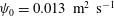 $\unicode[STIX]{x1D713}_{0}=0.013~\text{m}^{2}~\text{s}^{-1}$
. Other boundary conditions are chosen as free slip at the bottom, a solid wall with no-normal velocity at the right end boundary and the rigid lid at the top surface. The height and length of the computational domain are respectively
$\unicode[STIX]{x1D713}_{0}=0.013~\text{m}^{2}~\text{s}^{-1}$
. Other boundary conditions are chosen as free slip at the bottom, a solid wall with no-normal velocity at the right end boundary and the rigid lid at the top surface. The height and length of the computational domain are respectively
 $H=\unicode[STIX]{x03C0}$
m and the domain length is
$H=\unicode[STIX]{x03C0}$
m and the domain length is
 $L_{d}=15\unicode[STIX]{x1D706}_{1}+L_{m}\approx 125.513+L_{m}$
m where
$L_{d}=15\unicode[STIX]{x1D706}_{1}+L_{m}\approx 125.513+L_{m}$
m where
 $L_{m}\approx 0$
, 2.092 and 4.184 m. The length of the domain is chosen such that steady state can be reached. The domain is discretized with triangular elements with a total number of 33 290 triangles. Also, a second-order implicit scheme is employed for the time discretization of the wave equation.
$L_{m}\approx 0$
, 2.092 and 4.184 m. The length of the domain is chosen such that steady state can be reached. The domain is discretized with triangular elements with a total number of 33 290 triangles. Also, a second-order implicit scheme is employed for the time discretization of the wave equation.

Figure 5. Comparison of energy per unit area (
 $E^{\ast }$
) from analytical solution (——), FEM simulations (– – –), for respectively
$E^{\ast }$
) from analytical solution (——), FEM simulations (– – –), for respectively
 $L_{m}/\unicode[STIX]{x1D706}_{b}=0$
, 0.25 and 0.5 in (a), (b) and (c).
$L_{m}/\unicode[STIX]{x1D706}_{b}=0$
, 0.25 and 0.5 in (a), (b) and (c).

Figure 6. Effect of the wall reflectivity on the transmission (
 $T$
) and reflection (
$T$
) and reflection (
 $R$
) amplitudes and on the normalized energy per unit area
$R$
) amplitudes and on the normalized energy per unit area
 $\tilde{E}$
. Panels (a)–(c) respectively correspond to wall reflectivity of 100 % (i.e. perfect reflector and the same as figure 3
c), 50 % and 0 % (i.e. perfect absorber) and in all three cases
$\tilde{E}$
. Panels (a)–(c) respectively correspond to wall reflectivity of 100 % (i.e. perfect reflector and the same as figure 3
c), 50 % and 0 % (i.e. perfect absorber) and in all three cases
 $L_{m}/\unicode[STIX]{x1D706}_{b}=0.5$
which corresponds to the maximum
$L_{m}/\unicode[STIX]{x1D706}_{b}=0.5$
which corresponds to the maximum
 $\widetilde{E}$
at the end of the patch
$\widetilde{E}$
at the end of the patch
 $L=n\unicode[STIX]{x1D706}_{b}$
. Plotted in figures for
$L=n\unicode[STIX]{x1D706}_{b}$
. Plotted in figures for
 $T,R$
are mode 1 internal wave (——, blue), mode 3 (——, red), mode 5 (– – –, red), mode 7 (— ⋅ —, magenta) and mode 9 (——, black).
$T,R$
are mode 1 internal wave (——, blue), mode 3 (——, red), mode 5 (– – –, red), mode 7 (— ⋅ —, magenta) and mode 9 (——, black).
The comparison of spatial distribution of energy from theoretical predictions and those obtained by direct simulation from our FEM code is shown in figure 5 for
 $L_{m}/\unicode[STIX]{x1D706}_{b}=0$
, 0.25 and 0.50. In this figure,
$L_{m}/\unicode[STIX]{x1D706}_{b}=0$
, 0.25 and 0.50. In this figure,
 $E^{\ast }$
is the total energy normalized by the total energy of the incident wave (
$E^{\ast }$
is the total energy normalized by the total energy of the incident wave (
 $E_{\ell }$
) and is calculated as
$E_{\ell }$
) and is calculated as
 $E^{\ast }=(E^{k}+E^{p})/E_{\ell }$
, where the kinetic energy (
$E^{\ast }=(E^{k}+E^{p})/E_{\ell }$
, where the kinetic energy (
 $E^{k}$
) and the potential energy (
$E^{k}$
) and the potential energy (
 $E^{p}$
) are
$E^{p}$
) are
 $E^{k}=\sum _{n=1}^{\infty }1/2\unicode[STIX]{x1D70C}_{0}\int _{0}^{H}(\overline{u_{n}^{2}+w_{n}^{2}})\,\text{d}z$
and
$E^{k}=\sum _{n=1}^{\infty }1/2\unicode[STIX]{x1D70C}_{0}\int _{0}^{H}(\overline{u_{n}^{2}+w_{n}^{2}})\,\text{d}z$
and
 $E^{p}=\sum _{n=1}^{\infty }\int _{0}^{H}(g^{2}\overline{\unicode[STIX]{x1D70C}_{n}^{\prime 2}})/(2\unicode[STIX]{x1D70C}_{0}N^{2})\,\text{d}z$
(note that
$E^{p}=\sum _{n=1}^{\infty }\int _{0}^{H}(g^{2}\overline{\unicode[STIX]{x1D70C}_{n}^{\prime 2}})/(2\unicode[STIX]{x1D70C}_{0}N^{2})\,\text{d}z$
(note that
 $\widetilde{E}$
is the spatial average of
$\widetilde{E}$
is the spatial average of
 $E^{\ast }$
).
$E^{\ast }$
).
 $E^{\ast }$
is chosen here for validation because the horizontal spatial average (
$E^{\ast }$
is chosen here for validation because the horizontal spatial average (
 $\widetilde{E}$
) of the energy over the patch is not possible from numerical simulation results and would cause errors. Three ripples (instead of six as before) are chosen for validation because this requires a smaller domain and a smaller simulation time to reach steady state. As can be seen, theoretical predictions and direct simulation results show good agreement with each other.
$\widetilde{E}$
) of the energy over the patch is not possible from numerical simulation results and would cause errors. Three ripples (instead of six as before) are chosen for validation because this requires a smaller domain and a smaller simulation time to reach steady state. As can be seen, theoretical predictions and direct simulation results show good agreement with each other.
Clearly the amplification of the energy occurs due to the reflection from the wall and hence the observed energy directly depends on the reflectivity of the wall. The considered wall in this study is a simplified model for a finite-height ridge or a continental slope in real oceans, which have a finite height and hence cannot fully reflect the incident waves. This warrants the need to assess the effect of the reflectivity index on the energy amplification. To better understand this effect, we consider 3 different cases for which the reflectivity index
 $=$
100 % (perfect reflection), 50 % and 0 % (perfect absorption). This is shown in figure 6(a–c), where the transmission/reflection amplitudes of different modes and energy per unit area
$=$
100 % (perfect reflection), 50 % and 0 % (perfect absorption). This is shown in figure 6(a–c), where the transmission/reflection amplitudes of different modes and energy per unit area
 $\widetilde{E}$
are plotted for
$\widetilde{E}$
are plotted for
 $L_{m}/\unicode[STIX]{x1D706}_{b}=0.5$
which has the maximum energy amplification at the end of the patch
$L_{m}/\unicode[STIX]{x1D706}_{b}=0.5$
which has the maximum energy amplification at the end of the patch
 $\widetilde{E}(L_{m})$
. The first case of perfect reflection is the same as figure 3(c). As discussed previously, the transmission and reflection amplitudes are identical and
$\widetilde{E}(L_{m})$
. The first case of perfect reflection is the same as figure 3(c). As discussed previously, the transmission and reflection amplitudes are identical and
 $\widetilde{E}(L_{m})\approx 7$
. If the wall reflectivity index is 50 % (figure 6
b) then
$\widetilde{E}(L_{m})\approx 7$
. If the wall reflectivity index is 50 % (figure 6
b) then
 $\widetilde{E}(L_{m})\approx 3$
and both
$\widetilde{E}(L_{m})\approx 3$
and both
 $T$
and
$T$
and
 $R$
decrease while the decrease of the reflection amplitudes is more significant. Ultimately, zero reflectivity (i.e. the wall is a perfect absorber, figure 6
c), means that the wall has no role and it is identical to a single patch case (see figure 2). Here,
$R$
decrease while the decrease of the reflection amplitudes is more significant. Ultimately, zero reflectivity (i.e. the wall is a perfect absorber, figure 6
c), means that the wall has no role and it is identical to a single patch case (see figure 2). Here,
 $\widetilde{E}(L_{m})\approx 1.8$
and the transmission amplitude, especially the first mode attenuates compared to the other two cases. Also, as expected, all reflection amplitudes are fully zero at the wall and slightly increase towards the beginning of the patch. In order to further assess the impact of the reflectivity index on the energy distribution, the energy at the beginning
$\widetilde{E}(L_{m})\approx 1.8$
and the transmission amplitude, especially the first mode attenuates compared to the other two cases. Also, as expected, all reflection amplitudes are fully zero at the wall and slightly increase towards the beginning of the patch. In order to further assess the impact of the reflectivity index on the energy distribution, the energy at the beginning
 $\widetilde{E}(0)$
and end
$\widetilde{E}(0)$
and end
 $\widetilde{E}(L)$
of a six ripple patch is plotted in figure 7 as a function of reflectivity index, where
$\widetilde{E}(L)$
of a six ripple patch is plotted in figure 7 as a function of reflectivity index, where
 $L_{M}/\unicode[STIX]{x1D706}_{b}=0.5$
. The results show that with the increase of the reflectivity index the energy amplifies especially at the end of the patch. Results from figures 6 and 7 generally suggest that the strength of amplification has an algebraic dependence on the wall reflectivity index.
$L_{M}/\unicode[STIX]{x1D706}_{b}=0.5$
. The results show that with the increase of the reflectivity index the energy amplifies especially at the end of the patch. Results from figures 6 and 7 generally suggest that the strength of amplification has an algebraic dependence on the wall reflectivity index.

Figure 7. Variation of energy per unit area
 $\widetilde{E}$
at the beginning and end of a six ripple bottom patch (
$\widetilde{E}$
at the beginning and end of a six ripple bottom patch (
 $n_{r}=6$
) as a function of the wall reflectivity index. The energy
$n_{r}=6$
) as a function of the wall reflectivity index. The energy
 $\widetilde{E}$
is calculated for patch–wall distance of
$\widetilde{E}$
is calculated for patch–wall distance of
 $L_{m}/\unicode[STIX]{x1D706}_{b}=0.5$
.
$L_{m}/\unicode[STIX]{x1D706}_{b}=0.5$
.
We would like to briefly comment about the effect of viscosity here. Viscous dissipation within linear internal waves can be estimated by a linear approximation (Baines Reference Baines1998, § 4.7) and can be shown to be very small. For instance for a mode 1 internal wave under the parameters of the case presented in figure 5 and for a water depth of
 $H=100$
m, it can be shown that the rate of decay of vertical displacement is less than one per cent over the distance of 1000 km. Clearly if waves are steep, then nonlinear effects dominate the viscous dissipation and results potentially orders-of-magnitude different from the linear approximation may be obtained. In an extreme nonlinear case of the wave breaking, almost the entire energy of a wave is dissipated over a distance comparable to the wave’s wavelength (Gargett & Holloway Reference Gargett and Holloway1984; Lamb Reference Lamb2014).
$H=100$
m, it can be shown that the rate of decay of vertical displacement is less than one per cent over the distance of 1000 km. Clearly if waves are steep, then nonlinear effects dominate the viscous dissipation and results potentially orders-of-magnitude different from the linear approximation may be obtained. In an extreme nonlinear case of the wave breaking, almost the entire energy of a wave is dissipated over a distance comparable to the wave’s wavelength (Gargett & Holloway Reference Gargett and Holloway1984; Lamb Reference Lamb2014).
Turbulent (eddy) viscosity (
 $\unicode[STIX]{x1D708}_{t}$
) is much higher than molecular viscosity (
$\unicode[STIX]{x1D708}_{t}$
) is much higher than molecular viscosity (
 $\unicode[STIX]{x1D708}$
) in the ocean, especially in the mixed layer. However, it should be noted that the turbulent viscosity only bridges between the turbulent fluxes (i.e. turbulent momentum fluxes) and the mean shear rate (
$\unicode[STIX]{x1D708}$
) in the ocean, especially in the mixed layer. However, it should be noted that the turbulent viscosity only bridges between the turbulent fluxes (i.e. turbulent momentum fluxes) and the mean shear rate (
 $S$
). For example, in a one-dimensional flow
$S$
). For example, in a one-dimensional flow
 $\overline{u^{\prime }w^{\prime }}=-\unicode[STIX]{x1D708}_{t}S$
, where
$\overline{u^{\prime }w^{\prime }}=-\unicode[STIX]{x1D708}_{t}S$
, where
 $\overline{u^{\prime }w^{\prime }}$
is the turbulent momentum flux (Reynolds stress) and in our study
$\overline{u^{\prime }w^{\prime }}$
is the turbulent momentum flux (Reynolds stress) and in our study
 $S=\unicode[STIX]{x2202}\overline{U}/\unicode[STIX]{x2202}z$
where
$S=\unicode[STIX]{x2202}\overline{U}/\unicode[STIX]{x2202}z$
where
 $\overline{U}$
is the mean horizontal velocity and
$\overline{U}$
is the mean horizontal velocity and
 $z$
is the vertical distance from the reference at the bottom. Regardless of the value of the turbulent viscosity (
$z$
is the vertical distance from the reference at the bottom. Regardless of the value of the turbulent viscosity (
 $\unicode[STIX]{x1D708}_{t}$
), the fluxes are a function of
$\unicode[STIX]{x1D708}_{t}$
), the fluxes are a function of
 $S$
, which is low in our study so this consequently minimizes the production of the turbulent kinetic energy and turbulence effects and hence the dissipation of energy in the flow.
$S$
, which is low in our study so this consequently minimizes the production of the turbulent kinetic energy and turbulence effects and hence the dissipation of energy in the flow.
To assess the effect of viscosity on the mechanism elucidated in this article, we investigated the results of simulations, both inviscid and in the presence of viscosity with kinematic viscosity
 $\unicode[STIX]{x1D708}=10^{-6}$
,
$\unicode[STIX]{x1D708}=10^{-6}$
,
 $10^{-3}~\text{m}^{2}~\text{s}^{-1}$
, performed with the open source code SUNTANS (the Stanford unstructured non-hydrostatic terrain-following adaptive Navier–Stokes simulator). SUNTANS is a finite volume solver developed for simulation of three-dimensional non-hydrostatic internal waves in the ocean (Fringer, Gerritsen & Street Reference Fringer, Gerritsen and Street2006) and since its introduction in 2006, it has undergone cross-checks extensively (e.g. Fringer & Zhang Reference Fringer and Zhang2008; Wang et al.
Reference Wang, Fringer, Giddings and Fong2009; Kang & Fringer Reference Kang and Fringer2012). SUNTANS only uses a free surface boundary condition, and therefore does not completely agree with our theory (which is based on the rigid-lid assumption). However, it enables us to numerically study the effect of viscosity. The domain dimensions for our simulations are
$10^{-3}~\text{m}^{2}~\text{s}^{-1}$
, performed with the open source code SUNTANS (the Stanford unstructured non-hydrostatic terrain-following adaptive Navier–Stokes simulator). SUNTANS is a finite volume solver developed for simulation of three-dimensional non-hydrostatic internal waves in the ocean (Fringer, Gerritsen & Street Reference Fringer, Gerritsen and Street2006) and since its introduction in 2006, it has undergone cross-checks extensively (e.g. Fringer & Zhang Reference Fringer and Zhang2008; Wang et al.
Reference Wang, Fringer, Giddings and Fong2009; Kang & Fringer Reference Kang and Fringer2012). SUNTANS only uses a free surface boundary condition, and therefore does not completely agree with our theory (which is based on the rigid-lid assumption). However, it enables us to numerically study the effect of viscosity. The domain dimensions for our simulations are
 $H=100$
m and
$H=100$
m and
 $L=14\unicode[STIX]{x1D706}_{1}=3728.5$
m and chosen such that there is enough time for the steady state to be reached. The grid resolution is
$L=14\unicode[STIX]{x1D706}_{1}=3728.5$
m and chosen such that there is enough time for the steady state to be reached. The grid resolution is
 $1000\times 100$
in respectively the
$1000\times 100$
in respectively the
 $x$
and
$x$
and
 $z$
directions. Given the different domain dimensions between the FEM set-up and SUNTANS, the essential variables (such as bottom height to depth ratio,
$z$
directions. Given the different domain dimensions between the FEM set-up and SUNTANS, the essential variables (such as bottom height to depth ratio,
 $\unicode[STIX]{x1D707}$
, etc.) are chosen such that they match with the FEM set-up. Thus the three ripples have an amplitude of 4 m. The buoyancy frequency is chosen as
$\unicode[STIX]{x1D707}$
, etc.) are chosen such that they match with the FEM set-up. Thus the three ripples have an amplitude of 4 m. The buoyancy frequency is chosen as
 $N=0.0443~\text{s}^{-1}$
for an incident mode 1 wave with frequency
$N=0.0443~\text{s}^{-1}$
for an incident mode 1 wave with frequency
 $\unicode[STIX]{x1D714}=0.0266~\text{s}^{-1}$
and vertical wavenumber
$\unicode[STIX]{x1D714}=0.0266~\text{s}^{-1}$
and vertical wavenumber
 $m_{1}=0.0315~\text{m}^{-1}$
which result in the same
$m_{1}=0.0315~\text{m}^{-1}$
which result in the same
 $\unicode[STIX]{x1D707}$
as used in the FEM simulation. Also, the cross-shore velocity amplitude is
$\unicode[STIX]{x1D707}$
as used in the FEM simulation. Also, the cross-shore velocity amplitude is
 $U_{0}=0.013~\text{m}~\text{s}^{-1}$
. All the boundary conditions imposed in SUNTANS are similar to FEM simulation except the free surface on the top. As mentioned earlier, the free surface is used as the boundary condition in the numerical simulations because SUNTANS does not offer rigid-lid boundary condition. Our simulations show a maximum difference of less than 7 % between inviscid and viscous simulations with
$U_{0}=0.013~\text{m}~\text{s}^{-1}$
. All the boundary conditions imposed in SUNTANS are similar to FEM simulation except the free surface on the top. As mentioned earlier, the free surface is used as the boundary condition in the numerical simulations because SUNTANS does not offer rigid-lid boundary condition. Our simulations show a maximum difference of less than 7 % between inviscid and viscous simulations with
 $\unicode[STIX]{x1D708}=10^{-6}$
,
$\unicode[STIX]{x1D708}=10^{-6}$
,
 $10^{-3}~\text{m}^{2}~\text{s}^{-1}$
, confirming that the effect of viscosity is negligible for the current study.
$10^{-3}~\text{m}^{2}~\text{s}^{-1}$
, confirming that the effect of viscosity is negligible for the current study.
4.3 Two patch case
Now let us consider a second patch of ripples downstream of the patch under investigation (figure 1
b). For presentation purposes, we assume that the ripples in both patches have the same normalized wavenumber
 $n_{b}=2$
and amplitude
$n_{b}=2$
and amplitude
 $a_{b}=4\unicode[STIX]{x03C0}/100$
. The distribution of energy on each patch, and in the area between the two patches, similar to the case of § 4.2 is strongly dependent on
$a_{b}=4\unicode[STIX]{x03C0}/100$
. The distribution of energy on each patch, and in the area between the two patches, similar to the case of § 4.2 is strongly dependent on
 $L_{m}$
(the distance between the two patches). Distribution of energy density
$L_{m}$
(the distance between the two patches). Distribution of energy density
 $\widetilde{E}$
for
$\widetilde{E}$
for
 $L_{m}/\unicode[STIX]{x1D706}_{b}=0$
, 0.125, 0.250, 0.375 and 0.500 is shown in figure 8(a) for two identical patches of
$L_{m}/\unicode[STIX]{x1D706}_{b}=0$
, 0.125, 0.250, 0.375 and 0.500 is shown in figure 8(a) for two identical patches of
 $n_{r}=4$
seabed ripples. Note that the actual distance between the patch in each case is
$n_{r}=4$
seabed ripples. Note that the actual distance between the patch in each case is
 $q\unicode[STIX]{x1D706}_{b}+L_{m}$
(
$q\unicode[STIX]{x1D706}_{b}+L_{m}$
(
 $q$
positive integer) where in the case of figure 8(a),
$q$
positive integer) where in the case of figure 8(a),
 $q=4$
. But as before
$q=4$
. But as before
 $q$
does not play any role and it is
$q$
does not play any role and it is
 $L_{m}$
that determines the energy distribution. Figure 8(a) shows that for
$L_{m}$
that determines the energy distribution. Figure 8(a) shows that for
 $L_{m}/\unicode[STIX]{x1D706}_{b}=0$
, 0.125 and 0.250 energy continuously increases over two patches and is constant in the area between the two patches. For
$L_{m}/\unicode[STIX]{x1D706}_{b}=0$
, 0.125 and 0.250 energy continuously increases over two patches and is constant in the area between the two patches. For
 $L_{m}/\unicode[STIX]{x1D706}_{b}=0.375$
and 0.50,
$L_{m}/\unicode[STIX]{x1D706}_{b}=0.375$
and 0.50,
 $\widetilde{E}$
increases over the first patch, but decreases over the second patch in such a way that it gains a maximum in the area between the two patches: that is, energy is trapped in this area. To see the behaviour of the amplitude of each mode, we show in figure 8(b,c) the spatial evolution of the amplitudes of transmitted and reflected resonant modes (first five modes, i.e. modes 1, 3, 5, 7 and 9) over the two patches of ripples with
$\widetilde{E}$
increases over the first patch, but decreases over the second patch in such a way that it gains a maximum in the area between the two patches: that is, energy is trapped in this area. To see the behaviour of the amplitude of each mode, we show in figure 8(b,c) the spatial evolution of the amplitudes of transmitted and reflected resonant modes (first five modes, i.e. modes 1, 3, 5, 7 and 9) over the two patches of ripples with
 $L_{m}/\unicode[STIX]{x1D706}_{b}=0.50$
. Similar to the energy density, amplitudes of all modes consistently increase over the first patch, and in a similar way decrease over the second patch. Interestingly, at the end of the second patch, all the energy is back to the original incident wave energy: an upstream/downstream observer sees absolutely no trace of the two seabed patches on the upstream/downstream wave field.
$L_{m}/\unicode[STIX]{x1D706}_{b}=0.50$
. Similar to the energy density, amplitudes of all modes consistently increase over the first patch, and in a similar way decrease over the second patch. Interestingly, at the end of the second patch, all the energy is back to the original incident wave energy: an upstream/downstream observer sees absolutely no trace of the two seabed patches on the upstream/downstream wave field.

Figure 8. (a) The spatial evolution of energy density
 $\widetilde{E}$
in a two patch system with
$\widetilde{E}$
in a two patch system with
 $n_{r1}=n_{r2}=4$
(cf. figure 1) for different distances between the two patches
$n_{r1}=n_{r2}=4$
(cf. figure 1) for different distances between the two patches
 $L_{m}/\unicode[STIX]{x1D706}_{b}=0$
, 0.125, 0.25, 0.375 and 0.5. The normalized amplitude of seabed corrugations is 0.04. The maximum energy between the two patches is obtained when
$L_{m}/\unicode[STIX]{x1D706}_{b}=0$
, 0.125, 0.25, 0.375 and 0.5. The normalized amplitude of seabed corrugations is 0.04. The maximum energy between the two patches is obtained when
 $L_{m}/\unicode[STIX]{x1D706}_{b}=0.5$
and the maximum energy at the end of the second patch is obtained for
$L_{m}/\unicode[STIX]{x1D706}_{b}=0.5$
and the maximum energy at the end of the second patch is obtained for
 $L_{m}/\unicode[STIX]{x1D706}_{b}=0$
. (b,c) Spatial evolution of amplitude of the first five resonant modes (modes 1, 3, 5, 7 and 9) over the two patches of ripples with
$L_{m}/\unicode[STIX]{x1D706}_{b}=0$
. (b,c) Spatial evolution of amplitude of the first five resonant modes (modes 1, 3, 5, 7 and 9) over the two patches of ripples with
 $L_{m}/\unicode[STIX]{x1D706}_{b}=0.5$
. (d–f) Evolution of energy as a function of distance between two patches (d) at the beginning of the first patch, (e) between two patches and (f) at the end of the second patch.
$L_{m}/\unicode[STIX]{x1D706}_{b}=0.5$
. (d–f) Evolution of energy as a function of distance between two patches (d) at the beginning of the first patch, (e) between two patches and (f) at the end of the second patch.

Figure 9. (a) The spatial evolution of energy density
 $\widetilde{E}$
in a two patch system with
$\widetilde{E}$
in a two patch system with
 $n_{r1}=n_{r2}=4$
and
$n_{r1}=n_{r2}=4$
and
 $k_{b1}=2$
and
$k_{b1}=2$
and
 $k_{b2}=2.03$
(cf. figure 1) for different distances between the two patches
$k_{b2}=2.03$
(cf. figure 1) for different distances between the two patches
 $L_{m}/\unicode[STIX]{x1D706}_{b}=0$
, 0.125, 0.25, 0.375 and 0.5. The normalized amplitude of seabed corrugations is 0.04. (b,c) Spatial evolution of amplitude of the first five resonant modes (modes 1, 3, 5, 7 and 9) over the two patches of ripples with
$L_{m}/\unicode[STIX]{x1D706}_{b}=0$
, 0.125, 0.25, 0.375 and 0.5. The normalized amplitude of seabed corrugations is 0.04. (b,c) Spatial evolution of amplitude of the first five resonant modes (modes 1, 3, 5, 7 and 9) over the two patches of ripples with
 $L_{m}/\unicode[STIX]{x1D706}_{b}=0.5$
. (d) The spatial evolution of energy density
$L_{m}/\unicode[STIX]{x1D706}_{b}=0.5$
. (d) The spatial evolution of energy density
 $\widetilde{E}$
in a two patch system with
$\widetilde{E}$
in a two patch system with
 $n_{r1}=n_{r2}=4$
and
$n_{r1}=n_{r2}=4$
and
 $k_{b1}=2$
and
$k_{b1}=2$
and
 $k_{b2}=2.1$
for different distances between the two patches
$k_{b2}=2.1$
for different distances between the two patches
 $L_{m}/\unicode[STIX]{x1D706}_{b}=0$
, 0.125, 0.25, 0.375 and 0.5. (e,f) Spatial evolution of amplitude of the first five resonant modes (modes 1, 3, 5, 7 and 9) over the two patches of ripples with
$L_{m}/\unicode[STIX]{x1D706}_{b}=0$
, 0.125, 0.25, 0.375 and 0.5. (e,f) Spatial evolution of amplitude of the first five resonant modes (modes 1, 3, 5, 7 and 9) over the two patches of ripples with
 $L_{m}/\unicode[STIX]{x1D706}_{b}=0.5$
.
$L_{m}/\unicode[STIX]{x1D706}_{b}=0.5$
.
The behaviour of energy is also a function of the number of ripples in the patch as well as the number of ripples in the neighbouring patch. For a total number of ripples in both patches equal to
 $n_{r}=8$
, we show in figure 8(d–f) how energy density changes at the beginning of the first patch
$n_{r}=8$
, we show in figure 8(d–f) how energy density changes at the beginning of the first patch
 $\widetilde{E}(0)$
, between the two patches
$\widetilde{E}(0)$
, between the two patches
 $\widetilde{E}(n_{r1}\unicode[STIX]{x1D706}_{b})$
and at the end of the second patch
$\widetilde{E}(n_{r1}\unicode[STIX]{x1D706}_{b})$
and at the end of the second patch
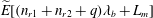 $\widetilde{E}[(n_{r1}+n_{r2}+q)\unicode[STIX]{x1D706}_{b}+L_{m}]$
. In all cases, energy at the beginning of the first and at the end of the second patch obtains a global minimum for
$\widetilde{E}[(n_{r1}+n_{r2}+q)\unicode[STIX]{x1D706}_{b}+L_{m}]$
. In all cases, energy at the beginning of the first and at the end of the second patch obtains a global minimum for
 $L_{m}/\unicode[STIX]{x1D706}_{b}=0.5$
. For the area between the two patches, energy is maximum for
$L_{m}/\unicode[STIX]{x1D706}_{b}=0.5$
. For the area between the two patches, energy is maximum for
 $L_{m}/\unicode[STIX]{x1D706}_{b}=0.5$
. The energy density upstream and downstream of the two patch system is only a function of the total number of ripples and not a function of how they are distributed in the two patches.
$L_{m}/\unicode[STIX]{x1D706}_{b}=0.5$
. The energy density upstream and downstream of the two patch system is only a function of the total number of ripples and not a function of how they are distributed in the two patches.
We also consider the effect of the change in the wavenumber of the second patch as shown in figure 9 for two cases where the second patch wavenumber is (i)
 $k_{b2}=2.03$
(left column) and (ii)
$k_{b2}=2.03$
(left column) and (ii)
 $k_{b2}=2.1$
(right column). Compared to figure 8, it can be seen that there is still an increase of energy between two patches, while the case where all the waves except the incident mode disappear is not observed.
$k_{b2}=2.1$
(right column). Compared to figure 8, it can be seen that there is still an increase of energy between two patches, while the case where all the waves except the incident mode disappear is not observed.
5 Concluding remarks
We presented here, analytically supported by direct simulation, that the energy distribution of internal waves over a patch of seabed undulations can be strongly dependent upon the distance of the patch to the neighbouring seabed features. Specifically, we considered two neighbouring features: a second patch of seabed undulations and a vertical wall (a perfect reflector). We showed that accumulation of internal waves energy may be an order of magnitude larger or smaller at specific areas of a patch, solely based on where the neighbouring feature is. The wall or the second patch, with specific properties and placement, can also completely cancel the effect of the first patch in such a way that upstream and downstream observers see no trace of the patch in their local wave field. The phenomenon elucidated here may influence, potentially significantly, the distribution of internal waves energy near steep oceanic ridges and continental slopes. In our case studies and simulations, without loss of generality, we considered an incident mode 1 internal wave. Similar results are obtained for an incident internal wave of any mode if proper conditions between the seabed and the incident internal wave hold.
It is worth noting that density stratification in real oceans is seldom linear and therefore
 $N$
is not constant and is in fact a function of the depth
$N$
is not constant and is in fact a function of the depth
 $z$
(e.g. Simpson Reference Simpson1971; Sigman, Jaccard & Haug Reference Sigman, Jaccard and Haug2004). The assumption of a linear density profile, nevertheless, is used extensively either as an approximation to the density profile in the ocean, or to extract the fundamental physics of internal waves (e.g. Thorpe Reference Thorpe1966; Klymak, Legg & Pinkel Reference Klymak, Legg and Pinkel2010; Lim, Ivey & Jones Reference Lim, Ivey and Jones2010; Bühler & Holmes-Cerfon Reference Bühler and Holmes-Cerfon2011; Li & Mei Reference Li and Mei2014; Guo & Holmes-Cerfon Reference Guo and Holmes-Cerfon2016). Although a nonlinear density profile affects the mode shapes of internal waves, the first-order Bragg reflection and hence the resonance condition are unaffected, i.e. for resonance to occur the topography wavenumber will still be twice as large as the wavenumber of the overpassing internal waves. Also, if the number of seabed undulations is large enough, the entire energy will be reflected. In a recent study, Liang, Zareei & Alam (Reference Liang, Zareei and Alam2017) studied the deviation from a linear density profile and it was shown that for parabolic and exponential profiles of density, the detuning of higher Bragg reflections from perfect resonance is negligible.
$z$
(e.g. Simpson Reference Simpson1971; Sigman, Jaccard & Haug Reference Sigman, Jaccard and Haug2004). The assumption of a linear density profile, nevertheless, is used extensively either as an approximation to the density profile in the ocean, or to extract the fundamental physics of internal waves (e.g. Thorpe Reference Thorpe1966; Klymak, Legg & Pinkel Reference Klymak, Legg and Pinkel2010; Lim, Ivey & Jones Reference Lim, Ivey and Jones2010; Bühler & Holmes-Cerfon Reference Bühler and Holmes-Cerfon2011; Li & Mei Reference Li and Mei2014; Guo & Holmes-Cerfon Reference Guo and Holmes-Cerfon2016). Although a nonlinear density profile affects the mode shapes of internal waves, the first-order Bragg reflection and hence the resonance condition are unaffected, i.e. for resonance to occur the topography wavenumber will still be twice as large as the wavenumber of the overpassing internal waves. Also, if the number of seabed undulations is large enough, the entire energy will be reflected. In a recent study, Liang, Zareei & Alam (Reference Liang, Zareei and Alam2017) studied the deviation from a linear density profile and it was shown that for parabolic and exponential profiles of density, the detuning of higher Bragg reflections from perfect resonance is negligible.
While practical aspects of the fundamental study presented here are beyond the scope of the current manuscript, we would like to briefly comment on some potential applications in real oceans. The oceanic internal wave spectrum ‘occupies a continuum in scales’, including a large number of waves with different frequencies and wavelengths which are clearly results of several mechanisms at play including what was discussed here (cf. Garrett & Munk Reference Garrett and Munk1972, Reference Garrett and Munk1975). Likewise, the seabed topography is typically irregular but can be decomposed into its Fourier components that in many cases have a few dominant peaks (Cox & Sandstrom Reference Cox and Sandstrom1962). Each Fourier component of the seabed, therefore, can resonate some of the waves in the internal waves spectrum through exact and near resonance mechanisms. Therefore, it may be expected that in real oceans with a broadband wave spectrum and a general irregular topography, multiple resonances occur at the same time leading to a complicated cascade of energy exchanged between modes and even chaos (e.g. Alam, Liu & Yue Reference Alam, Liu and Yue2009b , § 4.4).
Seabed features with periodic or near-periodic structures, as well, are found in many parts of the ocean (see e.g. Nicolas Reference Nicolas2013; Simarro et al.
Reference Simarro, Guillén, Puig, Ribó, Iacono, Palanques, Muñoz, Durán and Acosta2015). For example, the outer shelf of the east China sea (depth of
 $O(100)$
m) has sand ridges of tens of metres in amplitude spread over hundreds of kilometres. They are believed to have formed during the sea level rise some 10 000 years ago (Chang-shu & Jia-song Reference Chang-shu and Jia-song1988; Wu et al.
Reference Wu, Jin, Li, Zheng and Wang2005). Another example is the Sable Island bank off the coast of Nova Scotia that has a system of ridges of
$O(100)$
m) has sand ridges of tens of metres in amplitude spread over hundreds of kilometres. They are believed to have formed during the sea level rise some 10 000 years ago (Chang-shu & Jia-song Reference Chang-shu and Jia-song1988; Wu et al.
Reference Wu, Jin, Li, Zheng and Wang2005). Another example is the Sable Island bank off the coast of Nova Scotia that has a system of ridges of
 ${\sim}O(10)$
m tall, with a wavelength of
${\sim}O(10)$
m tall, with a wavelength of
 ${\sim}O(2000)$
m located in a water depth that reaches up to 80 m (Boczar-Karakiewicz, Amos & Drapeau Reference Boczar-Karakiewicz, Amos and Drapeau1990). At a larger scale, abyssal hills are ubiquitous, for instance covering some 80 % of the Pacific (abyssal hills are sometimes referred to as the most widespread topological features on the Earth Menard Reference Menard1964; Buck & Poliakov Reference Buck and Poliakov1998).
${\sim}O(2000)$
m located in a water depth that reaches up to 80 m (Boczar-Karakiewicz, Amos & Drapeau Reference Boczar-Karakiewicz, Amos and Drapeau1990). At a larger scale, abyssal hills are ubiquitous, for instance covering some 80 % of the Pacific (abyssal hills are sometimes referred to as the most widespread topological features on the Earth Menard Reference Menard1964; Buck & Poliakov Reference Buck and Poliakov1998).
Internal gravity waves have also been observed in a wide range of wavelengths. For instance, in the Baltic and North sea, there have been a number of observations of short-period internal waves with wavelengths of
 ${\sim}5000$
m with
${\sim}5000$
m with
 ${\sim}10$
m maximum vertical displacement, and off the coast of Japan, short internal waves have been reported with
${\sim}10$
m maximum vertical displacement, and off the coast of Japan, short internal waves have been reported with
 ${\sim}2000$
m wavelengths and 82 m maximum vertical displacement (see Roberts Reference Roberts1975, and references therein). In both areas, diurnal and semi-diurnal waves have also been observed and reported, but with much larger wavelengths.
${\sim}2000$
m wavelengths and 82 m maximum vertical displacement (see Roberts Reference Roberts1975, and references therein). In both areas, diurnal and semi-diurnal waves have also been observed and reported, but with much larger wavelengths.
Internal waves are well known to be significantly affected by seabed irregularities (e.g. Baines Reference Baines1998). The influence may be through linear and/or nonlinear mechanisms (e.g. resonance, instabilities, etc.). Internal waves, on the other hand, may be in charge in shaping sand ridges in the shallower waters of continental shelves in areas covered with sand and soft mud (e.g. Boczar-Karakiewicz et al. Reference Boczar-Karakiewicz, Amos and Drapeau1990). Internal waves are also known to (usually partially) reflect back from straight and steep slopes, unless in the case of critical reflection in which the reflected beam is along the slope and therefore does not carry energy away from the boundary (Cacchione & Wunsch Reference Cacchione and Wunsch1974; Eriksen Reference Eriksen1982; Maas et al. Reference Maas, Benielli, Sommeria and Lam1997).
The present study highlights the importance of coupling between these two effects: (i) internal waves scattering by the topography and (ii) the reflection from steep slopes. The trapping and amplification mechanism studied here may lead to spikes in the oceanic internal waves spectrum near continental slopes and steep oceanic ridges (e.g. 3 km tall Kaena Ridge in Hawaii (Klymak, Pinkel & Rainville Reference Klymak, Pinkel and Rainville2008)) that are next to small mean-seabed irregularities. As discussed above, in real ocean both internal waves and the seabed contain typically a broad band of wavenumbers. Since the phenomenon studied here is linear, therefore the effect of each Fourier mode of the seabed on corresponding mode(s) of the internal wave spectrum must be superimposed to obtain the overall picture.
Acknowledgements
This publication was made possible, in part, with the support of NSF (grant no. CBET-1414579-EAGER) and the American Bureau of Shipping. We would also like to thank the referees for their valuable comments.
Appendix A. Details of direct simulation implementation
A.1 Spatial and temporal discretization
We use FEM to solve for the streamfunction field in the whole domain. To that end, we first introduce an auxiliary variable
 $\unicode[STIX]{x1D719}$
and rewrite the governing equation as:
$\unicode[STIX]{x1D719}$
and rewrite the governing equation as:
 $$\begin{eqnarray}\displaystyle & \displaystyle \frac{\unicode[STIX]{x2202}^{2}\unicode[STIX]{x1D719}}{\unicode[STIX]{x2202}t^{2}}+N^{2}\frac{\unicode[STIX]{x2202}^{2}\unicode[STIX]{x1D713}}{\unicode[STIX]{x2202}x^{2}}=0, & \displaystyle\end{eqnarray}$$
 $$\begin{eqnarray}\displaystyle & \displaystyle \unicode[STIX]{x1D719}-\unicode[STIX]{x0394}\unicode[STIX]{x1D713}=0. & \displaystyle\end{eqnarray}$$
In order to solve for the unknown
 $(\unicode[STIX]{x1D719},\unicode[STIX]{x1D713})$
using FEM, we rewrite the system in its weak form using test function
$(\unicode[STIX]{x1D719},\unicode[STIX]{x1D713})$
using FEM, we rewrite the system in its weak form using test function
 $(\unicode[STIX]{x1D719}^{\ast },\unicode[STIX]{x1D713}^{\ast })$
. The variational formulation (after integration by parts) thus reads
$(\unicode[STIX]{x1D719}^{\ast },\unicode[STIX]{x1D713}^{\ast })$
. The variational formulation (after integration by parts) thus reads
 $$\begin{eqnarray}\displaystyle & & \displaystyle \iint _{\unicode[STIX]{x1D6FA}}\left[\frac{\unicode[STIX]{x2202}^{2}\unicode[STIX]{x1D719}}{\unicode[STIX]{x2202}t^{2}}\unicode[STIX]{x1D719}^{\ast }-N^{2}\frac{\unicode[STIX]{x2202}\unicode[STIX]{x1D713}}{\unicode[STIX]{x2202}x}\frac{\unicode[STIX]{x2202}\unicode[STIX]{x1D719}^{\ast }}{\unicode[STIX]{x2202}x}+\unicode[STIX]{x1D719}\unicode[STIX]{x1D713}^{\ast }+\unicode[STIX]{x1D735}\unicode[STIX]{x1D713}\boldsymbol{ : }\unicode[STIX]{x1D735}\unicode[STIX]{x1D713}^{\ast }\right]\text{d}\unicode[STIX]{x1D6FA}\nonumber\\ \displaystyle & & \displaystyle \quad +\int _{\unicode[STIX]{x2202}\unicode[STIX]{x1D6FA}}[N^{2}(\unicode[STIX]{x1D713}n_{x})\unicode[STIX]{x1D719}^{\ast }-(\unicode[STIX]{x1D735}\unicode[STIX]{x1D713}\boldsymbol{\cdot }\boldsymbol{n})\unicode[STIX]{x1D713}^{\ast }]\,\text{d}(\unicode[STIX]{x2202}\unicode[STIX]{x1D6FA})=0,\end{eqnarray}$$
where
 $\boldsymbol{n}$
is the outward normal vector to
$\boldsymbol{n}$
is the outward normal vector to
 $\unicode[STIX]{x2202}\unicode[STIX]{x1D6FA}$
and
$\unicode[STIX]{x2202}\unicode[STIX]{x1D6FA}$
and
 $\unicode[STIX]{x1D6FA}$
and
$\unicode[STIX]{x1D6FA}$
and
 $\unicode[STIX]{x2202}\unicode[STIX]{x1D6FA}$
are respectively the bulk and boundaries of the numerical domain. As the next step, this equation is discretized in time using a second-order implicit scheme. With the notation
$\unicode[STIX]{x2202}\unicode[STIX]{x1D6FA}$
are respectively the bulk and boundaries of the numerical domain. As the next step, this equation is discretized in time using a second-order implicit scheme. With the notation
 $(\unicode[STIX]{x1D719}(t_{n}),\unicode[STIX]{x1D713}(t_{n}))=(\unicode[STIX]{x1D719}_{n},\unicode[STIX]{x1D713}_{n})$
and the time step
$(\unicode[STIX]{x1D719}(t_{n}),\unicode[STIX]{x1D713}(t_{n}))=(\unicode[STIX]{x1D719}_{n},\unicode[STIX]{x1D713}_{n})$
and the time step
 $\unicode[STIX]{x1D6FF}t$
, the variational formulation thus becomes
$\unicode[STIX]{x1D6FF}t$
, the variational formulation thus becomes
 $$\begin{eqnarray}\displaystyle & & \displaystyle \iint _{\unicode[STIX]{x1D6FA}}\left[(\unicode[STIX]{x1D719}_{n+1}\unicode[STIX]{x1D719}^{\ast }-2\unicode[STIX]{x1D719}_{n}\unicode[STIX]{x1D719}^{\ast }+\unicode[STIX]{x1D719}_{n-1}\unicode[STIX]{x1D719}^{\ast })/2\unicode[STIX]{x1D6FF}t^{2}-\frac{N^{2}}{2}\left(\frac{\unicode[STIX]{x2202}\unicode[STIX]{x1D713}_{n+1}}{\unicode[STIX]{x2202}x}+\frac{\unicode[STIX]{x2202}\unicode[STIX]{x1D713}_{n-1}}{\unicode[STIX]{x2202}x}\right)\frac{\unicode[STIX]{x2202}\unicode[STIX]{x1D719}^{\ast }}{\unicode[STIX]{x2202}x}\right]\text{d}\unicode[STIX]{x1D6FA}\nonumber\\ \displaystyle & & \displaystyle \quad +\iint _{\unicode[STIX]{x1D6FA}}\left[\frac{1}{2}(\unicode[STIX]{x1D719}_{n+1}+\unicode[STIX]{x1D719}_{n-1})\unicode[STIX]{x1D713}^{\ast }+\frac{1}{2}\unicode[STIX]{x1D735}\unicode[STIX]{x1D713}_{n+1}\boldsymbol{ : }\unicode[STIX]{x1D735}\unicode[STIX]{x1D713}^{\ast }+\frac{1}{2}\unicode[STIX]{x1D735}\unicode[STIX]{x1D713}_{n-1}\boldsymbol{ : }\unicode[STIX]{x1D735}\unicode[STIX]{x1D713}^{\ast }\right]\text{d}\unicode[STIX]{x1D6FA}\nonumber\\ \displaystyle & & \displaystyle \quad +\int _{\unicode[STIX]{x2202}\unicode[STIX]{x1D6FA}}\left[\frac{N^{2}}{2}(\unicode[STIX]{x1D713}_{n+1}n_{x}+\unicode[STIX]{x1D713}_{n-1}n_{x})\unicode[STIX]{x1D719}^{\ast }-\frac{1}{2}(\unicode[STIX]{x1D735}\unicode[STIX]{x1D713}_{n+1}+\unicode[STIX]{x1D735}\unicode[STIX]{x1D713}_{n-1})\boldsymbol{\cdot }\boldsymbol{n}\unicode[STIX]{x1D713}^{\ast }\right]\text{d}(\unicode[STIX]{x2202}\unicode[STIX]{x1D6FA})=0.\qquad\end{eqnarray}$$
To close the system, we apply the following boundary conditions:
-
(i) The upper and lower boundaries are the streamlines
 $\unicode[STIX]{x1D713}_{n+1}=0$
at all times.
$\unicode[STIX]{x1D713}_{n+1}=0$
at all times. -
(ii) The inlet is a wavemaker generating a right-travelling incident mode 1 interval wave:
$\unicode[STIX]{x1D713}_{0}(z,t_{n})=\hat{\unicode[STIX]{x1D713}_{0}}\sin (k_{z}z)\cos (k_{x}x_{in}-\unicode[STIX]{x1D714}t_{n})$
. -
(iii) The outlet is a perfectly reflecting wall, i.e.
$u=0$
. Therefore,
$\unicode[STIX]{x1D713}$
is constant along the wall. Given that the wall intersects the upper and lower boundaries, we have
$\unicode[STIX]{x1D713}=0$
for the reflecting wall.


This equation is then projected on a set of shape functions (which are the same as the test functions) chosen as quadratic
 $P_{2}$
elements over the triangle which constitute the mesh. We apply a mesh refinement in the region close to the ripples and the wall, where the interactions between the internal waves and the domain features are important. The spatial discretization and the time resolution of the resulting discrete equations is done via the open source finite element solver FreeFem++ (Hecht Reference Hecht2012).
$P_{2}$
elements over the triangle which constitute the mesh. We apply a mesh refinement in the region close to the ripples and the wall, where the interactions between the internal waves and the domain features are important. The spatial discretization and the time resolution of the resulting discrete equations is done via the open source finite element solver FreeFem++ (Hecht Reference Hecht2012).
Note that the numerical domain is chosen long enough for the establishment of the steady state. A study of the inlet distance to the first ripples reveal that
 $L=15\unicode[STIX]{x1D706}_{1}$
is sufficient;
$L=15\unicode[STIX]{x1D706}_{1}$
is sufficient;
 $\unicode[STIX]{x1D706}_{1}$
being the wavelength of the incident mode 1 wave. Last, in order to observe Bragg reflection, the seabed corrugation has a wavelength
$\unicode[STIX]{x1D706}_{1}$
being the wavelength of the incident mode 1 wave. Last, in order to observe Bragg reflection, the seabed corrugation has a wavelength
 $\unicode[STIX]{x1D706}_{b}=\unicode[STIX]{x1D706}_{1}/2$
. We choose
$\unicode[STIX]{x1D706}_{b}=\unicode[STIX]{x1D706}_{1}/2$
. We choose
 $\unicode[STIX]{x1D6FF}t=0.1$
s (note that the scheme is unconditionally stable, but the precision depends on
$\unicode[STIX]{x1D6FF}t=0.1$
s (note that the scheme is unconditionally stable, but the precision depends on
 $\unicode[STIX]{x1D6FF}t$
) for which convergence is shown to occur and we solve for a time domain
$\unicode[STIX]{x1D6FF}t$
) for which convergence is shown to occur and we solve for a time domain
 $t\in [0,T]$
where
$t\in [0,T]$
where
 $T\sim 2L/C_{g}$
, with
$T\sim 2L/C_{g}$
, with
 $C_{g}$
the group velocity of mode 1 incident wave. In other words, we stop the simulation approximately when the incoming energy from the wavemaker has been reflected by the wall and returned to the inlet.
$C_{g}$
the group velocity of mode 1 incident wave. In other words, we stop the simulation approximately when the incoming energy from the wavemaker has been reflected by the wall and returned to the inlet.
A.2 Computation of the energy distribution
In order to compute the kinetic and potential energy distribution over the patch and compare with analytical predictions, we first need to obtain the velocity and density fields through the following (discretized) equations:
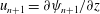 $u_{n+1}=\unicode[STIX]{x2202}\unicode[STIX]{x1D713}_{n+1}/\unicode[STIX]{x2202}z$
,
$u_{n+1}=\unicode[STIX]{x2202}\unicode[STIX]{x1D713}_{n+1}/\unicode[STIX]{x2202}z$
,
 $w_{n+1}=-\unicode[STIX]{x2202}\unicode[STIX]{x1D713}_{n+1}/\unicode[STIX]{x2202}x$
,
$w_{n+1}=-\unicode[STIX]{x2202}\unicode[STIX]{x1D713}_{n+1}/\unicode[STIX]{x2202}x$
,
 $\unicode[STIX]{x1D70C}_{n+1}^{\prime }=\unicode[STIX]{x1D70C}_{n-1}^{\prime }-(N^{2}\unicode[STIX]{x1D70C}_{o}/g)((\unicode[STIX]{x2202}\unicode[STIX]{x1D713}_{n+1}/\unicode[STIX]{x2202}x)+(\unicode[STIX]{x2202}\unicode[STIX]{x1D713}_{n-1}/\unicode[STIX]{x2202}x))\unicode[STIX]{x1D6FF}t$
where
$\unicode[STIX]{x1D70C}_{n+1}^{\prime }=\unicode[STIX]{x1D70C}_{n-1}^{\prime }-(N^{2}\unicode[STIX]{x1D70C}_{o}/g)((\unicode[STIX]{x2202}\unicode[STIX]{x1D713}_{n+1}/\unicode[STIX]{x2202}x)+(\unicode[STIX]{x2202}\unicode[STIX]{x1D713}_{n-1}/\unicode[STIX]{x2202}x))\unicode[STIX]{x1D6FF}t$
where
 $\unicode[STIX]{x1D70C}_{o}$
is the density at the free surface. At the steady state,
$\unicode[STIX]{x1D70C}_{o}$
is the density at the free surface. At the steady state,
 $E^{k}(x)$
and
$E^{k}(x)$
and
 $E^{p}(x)$
are the kinetic and potential energies of an internal wave integrated in the vertical
$E^{p}(x)$
are the kinetic and potential energies of an internal wave integrated in the vertical
 $z$
-direction. They are computed by averaging the instantaneous energies
$z$
-direction. They are computed by averaging the instantaneous energies
 $E_{n+1}^{k}$
and
$E_{n+1}^{k}$
and
 $E_{n+1}^{p}$
over the last
$E_{n+1}^{p}$
over the last
 $p$
-periods
$p$
-periods
 $T_{p}=p(2\unicode[STIX]{x03C0}/\unicode[STIX]{x1D714})$
(typically
$T_{p}=p(2\unicode[STIX]{x03C0}/\unicode[STIX]{x1D714})$
(typically
 $p=5$
). The integrals are approximated by a trapezoidal rule in time and a three-point Gauss quadrature in
$p=5$
). The integrals are approximated by a trapezoidal rule in time and a three-point Gauss quadrature in
 $z$
over each triangle edge adjacent to the vertical boundary, i.e.:
$z$
over each triangle edge adjacent to the vertical boundary, i.e.:
 $$\begin{eqnarray}\displaystyle & \!\displaystyle E^{k}(x)=\frac{1}{T_{p}}\mathop{\sum }_{t=0}^{t=T_{p}}\left\{\mathop{\sum }_{s=1}^{N_{t}}\mathop{\sum }_{g=1}^{3}\frac{\unicode[STIX]{x1D70C}_{o}}{2H}\left[\frac{w_{n+1}(z_{g})^{2}+w_{n}(z_{g})^{2}}{2}+\frac{u_{n+1}(z_{g})^{2}+u_{n}(z_{g})^{2}}{2}\right]\!\unicode[STIX]{x1D6FD}_{g}\right\}\unicode[STIX]{x1D6FF}t\qquad & \displaystyle\end{eqnarray}$$
 $$\begin{eqnarray}\displaystyle & \!\displaystyle E^{p}(x)=\frac{1}{T_{p}}\mathop{\sum }_{t=0}^{t=T_{p}}\left\{\mathop{\sum }_{s=1}^{N_{t}}\mathop{\sum }_{g=1}^{3}\frac{g^{2}}{2H\unicode[STIX]{x1D70C}_{o}N^{2}}\left[\frac{\unicode[STIX]{x1D70C}_{n+1}^{\prime }(z_{g})^{2}+\unicode[STIX]{x1D70C}_{n}^{\prime }(z_{g})^{2}}{2}\right]\!\unicode[STIX]{x1D6FD}_{g}\right\}\unicode[STIX]{x1D6FF}t,\qquad & \displaystyle\end{eqnarray}$$
where
 $z_{g}$
and
$z_{g}$
and
 $\unicode[STIX]{x1D6FD}_{g}$
are respectively the Gauss quadrature points and their associated weights. Here
$\unicode[STIX]{x1D6FD}_{g}$
are respectively the Gauss quadrature points and their associated weights. Here
 $N_{t}=38$
is the number of triangle edges used to discretize the inlet lateral boundary.
$N_{t}=38$
is the number of triangle edges used to discretize the inlet lateral boundary.


