2.1. Governing equations and numerical model

The governing equations are non-dimensionalised using typical scales for the study of KH instabilities, with tildes denoting the dimensional forms of distance $\boldsymbol {x}=(x,y,z)$, time, $t$, velocity, $\boldsymbol {u}=(u,v,w)$, density, $\rho$, tracer concentration, $\phi$, and pressure, $p$,

\begin{gather*} x = \tilde{x}/h,\quad y = \tilde{y}/h,\quad z = \left(\tilde{z}-z_0\right)/h,\quad t = \tilde{t}U_0/h, \quad \boldsymbol{u} = \tilde{\boldsymbol{u}}/U_0, \\ \rho = \left(\tilde{\rho}-\rho_0\right)/{\rm \Delta}\rho, \quad \phi =\tilde{\phi}/{\rm \Delta}\phi, \quad p = \tilde{p} / \rho_0 U_0^2. \end{gather*}

The dimensional parameters used here are the value defining the width of the pycnocline and the shear layer, $h$, the midpoint of the stratification and shear layer, $z_0$, half of the change in velocity across the two layers, $U_0$, the density at the midpoint of the density distribution, $\rho _0$, half of the change in density across the two layers, ${\rm \Delta} \rho$, and the maximum initial tracer concentration, ${\rm \Delta} \phi$. Using these dimensionless variables, the continuity equation and equations of conservation of momentum, density and passive tracer can be written in their incompressible and Boussinesq forms as

(2.1a)\begin{gather} \boldsymbol{\nabla} \boldsymbol{\cdot} \boldsymbol{u} = 0, \end{gather}

(2.1b)\begin{gather}{\partial \boldsymbol{u}}/{\partial t} + \boldsymbol{\boldsymbol{u}}\boldsymbol{\cdot}\boldsymbol{\nabla}\boldsymbol{u} ={-}\boldsymbol{\nabla} p - {Ri}_0 \rho \boldsymbol{\hat{k}} + {Re}_0^{{-}1} \nabla^2 \boldsymbol{u}, \end{gather}

(2.1c)\begin{gather}{\partial \rho}/{\partial t} + \boldsymbol{\boldsymbol{u}}\boldsymbol{\cdot}\boldsymbol{\nabla}\rho = ({Re}_0 {Pr})^{{-}1} \nabla^2 \rho, \end{gather}

(2.1d)\begin{gather}{\partial \phi}/{\partial t} + \boldsymbol{\boldsymbol{u}}\boldsymbol{\cdot}\boldsymbol{\nabla}\phi = ({Re}_0 {Sc})^{{-}1} \nabla^2 \phi, \end{gather}

with $\boldsymbol {\hat {k}}$ denoting the unit vector of the vertical axis. The dimensionless parameters included in these equations are the initial Reynolds number, ${Re}_0 = U_0 h /\nu$, the Prandtl number, ${Pr} = \nu /\kappa _\rho$, and the Schmidt number, ${Sc} = \nu /\kappa _\phi$, where $\nu$ is the kinematic viscosity, and $\kappa _{\rho }$ and $\kappa _{\phi }$ are the prescribed molecular diffusivity constants for density and the passive tracer, respectively. ${Ri}_0$ is the minimum initial Richardson number, which follows the standard definition for the gradient Richardson number,

(2.2)\begin{equation} {Ri} ={-}\frac{g}{\rho_0}\frac{\dfrac{\partial \tilde{\rho}}{\partial \tilde{z}}}{\left(\dfrac{\partial \tilde{u}}{\partial \tilde{z}}\right)^2}, \end{equation}

and can be expressed as

(2.3)\begin{equation} {Ri}_0 \approx \frac{g {\rm \Delta} \rho h}{\rho_0U_0^2}, \end{equation}

based on the initial conditions presented in the following section. The configuration parameters are chosen so that the necessary criterion for stratified shear instability, ${Ri}_0 < 1/4$, is satisfied. For the sake of completeness, relevant dimensional parameters prescribed in the simulations presented in this paper are given in table 2 in appendix A.

The numerical simulations presented in this paper were performed using the non-hydrostatic, non-Boussinesq version of the Coastal and Regional Ocean Community model (CROCO). This model was adapted from the Regional Ocean Modeling System (ROMS, Shchepetkin & McWilliams Reference Shchepetkin and McWilliams2005) to include non-hydrostatic and compressible effects (Auclair et al. Reference Auclair, Bordois, Dossmann, Duhaut, Paci, Ulses and Nguyen2018). While numerical simulations of KH instabilities are often considered in a periodic domain with free-slip rigid lid conditions for the upper and lower boundaries (e.g. Mashayek & Peltier Reference Mashayek and Peltier2012b, Reference Mashayek and Peltier2013), the implementation presented here utilises a free-surface upper boundary, and a flat, solid, bottom boundary, with periodic lateral boundary conditions in the $x$- and $y$-directions (streamwise and spanwise directions, respectively). The existence of a free surface and compressibility adds two dynamical processes (surface and acoustic waves) compared to more traditional studies of KH instabilities in incompressible, unbounded or rigid lid flows. It has been verified that, with the chosen configurations where the instability develops far from the vertical boundaries, the impact of these additional processes on the results is negligible when compared to the traditional configuration (see appendix A for further details regarding the implementation of CROCO and the discussion in the concluding section). However, in certain circumstances, surface and acoustic waves may play a role in modifying the turbulent cascade (see, for example, Shete & Guha Reference Shete and Guha2018).

2.2. Initial conditions

The initial conditions (ICs) for the simulations presented in this paper follow those from previous numerical studies of Kelvin–Helmholtz instabilities (e.g. Salehipour, Peltier & Mashayek Reference Salehipour, Peltier and Mashayek2015). In their dimensionless forms, the extents of the domain in the streamwise, spanwise and vertical directions are given by $L_x$, $L_y$ and $L_z$, respectively. Both two-dimensional (2-D) and three-dimensional (3-D) configurations are examined, with periodic boundary conditions in the horizontal directions, a flat, free-slip, rigid bottom and a free surface in the vertical direction. The initial density distribution is defined as two constant-density layers separated by a strongly stratified pycnocline, with a weak stable background stratification superimposed,

(2.4)\begin{equation} \rho\left( \boldsymbol{x},0 \right) ={-}\beta z - \tanh(z). \end{equation}

The linear background term $\beta z$ is a minor modification to the standard configuration for the purpose of defining the scatter plots in density–tracer space discussed in § 4.1 over the entire vertical domain in physical space (i.e. each density value initially corresponds to a unique value of height). Note that the definition of the initial Richardson number (2.3) ignores the weak linear background term of the initial density profile, since it was confirmed to have a negligible influence on the development of the instability when compared to the initial stratification without the weak linear background ($\beta \approx 3.5\times 10^{-3} \ll 1$ in this study).

The initial velocity field is given by

(2.5)\begin{equation} \left.\begin{array}{c@{}}u\left( \boldsymbol{x}, t=0 \right) = U\left(z\right) + u^\prime(\boldsymbol{x}), \\ v\left( \boldsymbol{x}, t=0 \right) = v^\prime(\boldsymbol{x}), \\ w\left( \boldsymbol{x}, t=0 \right) = w^\prime(\boldsymbol{x}).\end{array}\right\} \end{equation}

Here, $U(z)$ is the initial background flow providing the shear and is defined by a hyperbolic tangent profile, with the upper layer moving leftward, and the lower layer moving rightward,

(2.6)\begin{equation} U(z) ={-}\tanh\left(z\right). \end{equation}

and $u^\prime$, $v^\prime$ and $w^\prime$ are small amplitude perturbations, required to kickstart the instability, defined as

(2.7)\begin{gather} u^\prime(x,y,z) = \epsilon f^\prime(z)\sin\left(\frac{2{\rm \pi} n_x}{L_x}x\right) \left(1+\epsilon_{3\hbox{-}\mathrm{D}}\sin\left(\frac{2{\rm \pi} n_y}{L_y}y\right)\right), \nonumber\\ v^\prime(x,y,z) = 0, \nonumber\\ w^\prime(x,y,z) ={-}\epsilon f(z)\frac{2{\rm \pi} n_x}{L_x}\cos\left(\frac{2{\rm \pi} n_x}{L_x}x\right)\left(1+\epsilon_{3\hbox{-}\mathrm{D}}\sin\left(\frac{2{\rm \pi} n_y}{L_y}y\right)\right). \end{gather}

This choice of functional form for the perturbation ensures that the initial velocity field is non-divergent, which is important in the context of this numerical implementation. The function

(2.8)\begin{equation} f(z) = 1 - \tanh^2\left(\frac{z}{\alpha}\right), \end{equation}

ensures that the initial perturbation is localised within the region of the shear, with $\alpha = 4.29$; $\epsilon =0.01$ is a dimensionless parameter that sets the magnitude of the perturbation in the streamwise direction, while $n_x$ and $n_y$ set the wavelengths of the initial perturbation in the $x$- and $y$-directions, respectively; $\epsilon _{\mathrm {3D}}$ sets the magnitude of the spanwise perturbations, and for 3-D configurations, $\epsilon _{\mathrm {3D}}=0.2$. For 2-D configurations, both $n_y=0$ and $\epsilon _{\mathrm {3D}}=0$.

In addition to the dynamical fields, passive tracer fields are defined by an initial profile of the form

(2.9)\begin{equation} \phi\left( \boldsymbol{x},0 \right) = a{\textrm{sech}}^2\left(az - b\right), \end{equation}

where $a$ is a dimensionless parameter that determines the width of the tracer distribution, while ensuring the total amount of tracer remains constant between simulations, and $b$ indicates the offset of the tracer from the pycnocline. The tracer is thus initially distributed in a layer, with its maximum initial value located at $z=b/a$. Both the vertical position and the width of the tracer layer will be varied in simulations presented later in this paper, but for the different dynamical configurations discussed first in § 2.3, the tracer layer is collocated with the midpoints of the stratification and the shear ($b=0$), and the maximum initial tracer value is $1$ ($a=1$). Sketches of the initial vertical profiles of the shear, density and passive tracer fields are depicted in figure 1, with associated dimensional parameters.

Figure 1. (Left to right) Initial vertical profiles of the velocity, density, and passive tracer fields for the described simulations with relevant dimensional parameters.

2.3. Description of dynamical configurations

The primary experiment presented in this section compares simulations of three different dynamical configurations, all with identical initial background fields and prescribed parameters. The relevant dimensionless parameters used in all simulations are ${Ri}_0 = 0.1158$, ${Re} = 2000$, ${Pr} = 1$ and ${Sc} = 1$. The non-dimensional wavelength of the fastest-growing mode as predicted by the Taylor–Goldstein equations for these given initial background velocity and density profiles is $\lambda _{{KH}}\approx 14.3$. As such, the length of the domain is the streamwise direction was chosen as $L_x=\lambda _{{KH}}$, so that a single KH billow develops, or $L_x=2~\lambda _{{KH}}$, so that two KH billows develop, possibly leading to pairing in 2-D configurations. The parameters $N_x$, $N_y$ and $N_z$ are the number of grid points in the streamwise, spanwise and vertical directions, respectively. Combined with the length of the domain in each direction, this leads to a consistent dimensionless grid spacing in the $x$-, $y$- and $z$-directions of ${\rm \Delta} x = {\rm \Delta} y = {\rm \Delta} z = 0.0559$. ${\rm \Delta} t$ is the dimensionless barotropic time step. Table 1 presents the parameters that vary between each dynamical configuration. Additional parameters relevant to the non-Boussinesq components of the model are listed in appendix A. The three dynamical configurations are defined as follows:

1. (i) Configuration I is 2-D, with $L_x=\lambda _{{KH}}$ and $n_x=1,\ n_y=0$ (so that $v=0$ at all times). The initial perturbation corresponds to the most unstable wavelength and only one billow develops in this simulation.

2. (ii) Configuration II is also 2-D, except that $L_x=2~\lambda _{{KH}}=L_z$ and $n_x=2$. The length of the domain and wavelength of the perturbation allow for the formation of two billows, which eventually give way to pairing and additional mixing.

3. (iii) Configuration III is 3-D, with spanwise parameters $L_y=0.375~\lambda _{{KH}}$, $n_y=4$, while the streamwise and vertical parameters are the same as configuration I ($L_x=\lambda _{{KH}}$, $n_x=1$). This allows for mixing by spanwise secondary instabilities that lead to the breakdown of the primary KH billow.

Table 1. Relevant computational parameters of the three dynamical configurations presented in this paper.

Due to the inclusion of the third dimension and resulting spanwise instabilities, configuration III provides a more realistic simulation than the other two cases. Configurations I and II, while less physically realistic, provide additional pathways to turbulence and mixing, despite showing nearly identical initial behaviour. Comparing the three configurations therefore permits the evaluation of the impact of the route to turbulence on tracer mixing.

3.1. Evolution of the different dynamical configurations

In order to follow the time evolution of the three dynamical configurations, the mean background and perturbation kinetic energy (KE) are defined in the standard way (e.g. Mashayek & Peltier Reference Mashayek and Peltier2013). This requires definitions for the mean background and perturbation velocity fields. The mean background velocity field is a function of $z$ only, and is given as

(3.1)\begin{equation} \overline{\boldsymbol{u}}(z) = \frac{1}{L_xL_y}\iint \boldsymbol{u}\,\textrm{d} x\,\textrm{d} y. \end{equation}

The 2-D velocity perturbation is a function of $x$ and $z$, defined as

(3.2)\begin{equation} \boldsymbol{u}_{2\hbox{-}\mathrm{D}} = \frac{1}{L_y}\int \left(\boldsymbol{u}-\overline{\boldsymbol{u}}\left(z\right)\right)\textrm{d} y. \end{equation}

Finally, the 3-D velocity perturbation can be expressed using the background velocity and the 2-D velocity perturbation,

(3.3)\begin{equation} \boldsymbol{u}_{3\hbox{-}\mathrm{D}} = \boldsymbol{u}-\boldsymbol{u}_{2\hbox{-}\mathrm{D}}-\overline{\boldsymbol{u}}\left(z\right). \end{equation}

Following these definitions, the background KE, KE due to 2-D perturbations, and KE due to the 3-D perturbations are defined as

(3.4)\begin{gather} \overline{\mathcal{K}} = \frac{1}{L_z}\int \frac{\overline{\boldsymbol{u}}^2}{2}\,\textrm{d} z, \end{gather}

(3.5)\begin{gather}\mathcal{K}_{2\hbox{-}\mathrm{D}} = \frac{1}{L_x L_z}\iint \frac{\boldsymbol{u}_{2\hbox{-}\mathrm{D}}^2}{2}\,\textrm{d} x\,\textrm{d} z, \end{gather}

(3.6)\begin{gather}\mathcal{K}_{3\hbox{-}\mathrm{D}} = \frac{1}{L_x L_y L_z}\iiint \frac{\boldsymbol{u}_{3\hbox{-}\mathrm{D}}^2}{2}\,\textrm{d} x\,\textrm{d} y\,\textrm{d} z, \end{gather}

respectively, noting that the mean KE can be expressed as the sum of these three values,

(3.7)\begin{equation} \mathcal{K} = \frac{1}{V}\int \frac{\boldsymbol{u}^2}{2}\,\textrm{d} V = \overline{\mathcal{K}} + \mathcal{K}_{2\hbox{-}\mathrm{D}} + \mathcal{K}_{3\hbox{-}\mathrm{D}}. \end{equation}

The general evolution of the dynamical configurations is tracked in figure 2, which plots their mean KE as functions of time. Note that although each of the simulations are performed on domains with different volumes, the initial mean KE is identical for all three cases. This provides a straightforward depiction of the divergent behaviour between the three cases. The 2-D and 3-D perturbation KE will be discussed further in § 4.2 when discussing tracer mixing.

Figure 2. Time evolution of the mean KE $\mathcal {K}$ for configuration I (dashed line), configuration II (solid line) and configuration III (dotted line). The labelled times correspond to the rows of cross-sections plotted in figures 3 and 4.

Figures 3 and 4 present the evolution of the density and passive tracer, respectively, for the three dynamical configurations. Each row corresponds to a specific time depicted on the KE time series of figure 2, which indicates an important stage in KH development, or points at which the development of the configurations diverge. The distinct phases enumerated in figure 2 are as follows:

1. (i) The initial period of linear growth, as predicted by inviscid Taylor–Goldstein theory. This phase is nearly identical for all three simulations, although some weak spanwise effects are visible in the 3-D simulation. Each simulation exhibits stirring of the low and high-density regions by 2-D KH billows with a wavelength close to that of the fastest-growing mode predicted by Taylor–Goldstein theory.

2. (ii) The branching point between 2-D and 3-D simulations due to the onset of secondary instabilities. All three configurations exhibit secondary shear instabilities along the tilted pycnocline, and secondary convective instabilities within the vortices, while spanwise instabilities begin to emerge in the 3-D configuration. The density field develops alternating layers of high and low density, while the passive tracer takes the shape of ellipses with maximum values centred within the billows, gradually decreasing to no tracer at the billow exterior. A thin strand of low tracer concentration occurs along the braids, while even lower concentrations of tracer are visible between the horizontal edges of the billows.

3. (iii) First onset of small-scale features, resulting to greater mixing in all simulations. In the 2-D configurations, this leads to the density within the billows becoming nearly uniform. In the 3-D configuration, this leads to a wider pycnocline that is no longer unstable to shear instabilities. The 2-D cases keep their tracer maxima focused at the centre of the billows, although some tracer is pulled from the high concentration regions towards the outsides of the billows. Meanwhile, the density field experiences greater mixing due to the appearance of the small-scale features, and becomes nearly homogeneous within the billows. The secondary instabilities in configuration III mix the high tracer concentration region at the centre of the billow, redistributing the tracer throughout the rest of the pycnocline.

4. (iv) The onset of pairing in configuration II, which results in much greater mixing further into the low- and high-density layers, while mixing the concentrated regions of tracer within the two billows with the regions external to the billows without tracer. The single billow of configuration I maintains a nearly constant shape and size.

5. (v) Second onset of small scales due to enhanced stretching from the pairing in configuration II. Configuration III has reached an essentially steady state.

6. (vi) The nearly steady final phase of the 2-D configurations. The single billow of configuration I continuously rolls and experiences slow diffusion of density at the edges of the vortex. The pairing of configuration II induces stretching, causing new small-scale instabilities to develop, and enhancing the homogenisation of tracer fields within the billows. This leads to formation of a single larger billow that eventually remains nearly steady.

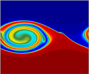
Figure 3. Evolution of slices of the density field for configurations I (a–f), II (g–l) and III (in the streamwise (m–q) and spanwise (r–v) directions) at the times indicated in figure 2. The dashed lines in the images of the third column indicate the position of the spanwise slices depicted in the fourth column, while the streamwise slices of the third column correspond to the right edge of the spanwise slices.

Figure 4. Evolution of slices of the passive tracer field for configurations I (a–f), II (g–l) and III (in the streamwise (m–q) and spanwise (r–v) directions) at the times indicated in figure 2. The dashed lines in the images of the third column indicate the position of the spanwise slices depicted in the fourth column, while the streamwise slices of the third column correspond to the right edge of the spanwise slices.

4.1. Weighted density–tracer scatter plots

For definiteness, mixing is here defined as an irreversible process during which the density or tracer concentration of a given fluid parcel is modified. In the equations (2.1c) and (2.1d), it is allowed by the inclusion of an explicit diffusion term. Following other papers on this topic, the term diabatic is used to denote an irreversible (and correspondingly adiabatic to denote a reversible) process applying to density. Stirring is the process of geometric deformation of fluid elements that leads to diffusive mixing, but before diffusion acts. It is in principle reversible, because it does not change the density or tracer concentration within fluid elements. To characterise the diapycnal mixing of tracers during a dynamical event, scatter plots which show the characteristics of fluid parcels in terms of their location in a 2-D space in which the coordinates are density ($\rho$) and tracer concentration ($\phi$) are employed. In such plots, a fluid parcel will remain at the same position in density–tracer ($\rho \phi$) space whatever its displacement or geometrical deformation in physical space, provided that there is no irreversible mixing due to the action of diffusion. Any change in the distribution of fluid parcels in $\rho \phi$ space is therefore indicative that irreversible mixing has occurred. Similar diagrams are often used to characterise mixing in geophysical flows, such as temperature–salinity diagrams used to qualify the mixing of large water masses in the ocean (e.g. Tomczak Reference Tomczak1981; Teramoto Reference Teramoto1993); tracer–salinity estuarine mixing curves used to identify whether an estuary may act as a source or sink of a given tracer (e.g. Loder & Reichard Reference Loder and Reichard1981; Officer & Lynch Reference Officer and Lynch1981); or tracer–tracer diagrams used to examine compact relationships between different atmospheric tracers (e.g. Tilmes et al. Reference Tilmes, Müller, Grooß, Nakajima and Sasano2006; Plumb Reference Plumb2007). Scatter plots are thus convenient for the purpose of the analysis presented here as they permit the straightforward identification of diapycnal tracer transport which must be indicated by the generation of new points in density–tracer space. For example, if the density–tracer distribution is initially given by the solid black line in figure 5, then the evolution to a distribution given by the dashed line is indicative of diapycnal tracer flux.

Figure 5. Sketch of the initial scatter plot of tracer as a function of density associated with the profiles given by (2.4) and (2.9) where the pycnocline and tracer layer are collocated (solid line). Hypothetical evolution of the scatter plot after a mixing event showing diapycnal fluxes of tracer (dashed line). In the new profile, mixing has led to a flux of tracer towards lower densities.

The geometry of density–tracer scatter plots does not by itself uniquely define density and tracer distributions in physical space. Further information is provided by associating each point in density–tracer space with a ‘weight’, which is a discrete formulation of the density–tracer probability function presented in appendix D of Plumb (Reference Plumb2007), which quantifies the amount of fluid in a given density–tracer bin. The procedure to calculate the weight is outlined as follows. The density and tracer domains are subdivided into $N_\rho$ and $N_\phi$ individual bins, respectively, with sizes

(4.1)\begin{gather} \delta\rho=\frac{\rho_{Max}-\rho_{Min}}{N_\rho}, \end{gather}

(4.2)\begin{gather}\delta\phi=\frac{\phi_{Max}-\phi_{Min}}{N_\phi}, \end{gather}

where the subscripts ${Max}$ and ${Min}$ indicate the maximum and minimum values of the density and the tracer. The centre of a given bin is defined by the point $(\rho _i,\phi _j)$, where

(4.3)\begin{gather} \rho_i=\rho_{Min}+\frac{2i - 1}{2}\delta\rho,\quad i=1,2,\ldots,N_\rho, \end{gather}

(4.4)\begin{gather}\phi_j=\phi_{Min}+\frac{2j - 1}{2}\delta\phi,\quad j=1,2,\ldots,N_\phi. \end{gather}

The weight corresponding to a given bin with centre $(\rho _i,\phi _j)$, $W_{ij}(t)$, is calculated as

(4.5)\begin{align} W_{ij}\left(t\right) &= W\left(\rho_i,\phi_j,t\right) \nonumber\\ &= \frac{1}{V} \sum I_{ij}(\rho,\phi,t) {\rm \Delta} V, \end{align}

where ${\rm \Delta} V = {\rm \Delta} x \times {\rm \Delta} y \times {\rm \Delta} z$, and

(4.6)\begin{align} I_{ij}(\rho,\phi,t) = \left\{\begin{array}{@{}ll} 1, & \left(\rho\left(\boldsymbol{x},t\right) - \rho_i,\phi\left(\boldsymbol{x},t\right) - \phi_j\right) \in \left[- \dfrac{1}{2}\delta\rho,\dfrac{1}{2}\delta\rho\right) \times \left[- \dfrac{1}{2}\delta\phi, \dfrac{1}{2}\delta\phi\right)\\ 0, & {\rm otherwise}, \end{array}\right. \end{align}

and its value is represented in colour on the scatter plot. Note that the total weight is conserved (i.e. the total is always 1), and the integral of the weight multiplied by the tracer concentration or density is also conserved in the absence of sources and sinks.

Since graphical limitations can make it difficult to discern when a scatter plot has converged to a compact relationship, it is useful to define a diagnostic that acts as a measure of the scatter,

(4.7)\begin{equation} R\left(t\right)=\frac{\int\left(\phi(\boldsymbol{x},t) - \phi_*(z,t)\right)^2 \textrm{d} V}{\int\left(\phi(\boldsymbol{x},t) - \overline{\phi}\right)^2\textrm{d} V}. \end{equation}

This value will be referred to as the scatter variance. It relates the total variance of the tracer from the isopycnal mean $\phi _*$ (as defined by (C 11) in appendix C) to the total variance of tracer from the mean over the whole domain $\overline {\phi }$. As such, it presents a time evolution of the scatter plots, with larger values of $R$ indicating greater relative variance over a given density bin, and smaller values indicating a convergence towards functional, compact relationships between $\rho$ and $\phi$.

4.2. Scatter plot evolution for the different dynamical configurations

Figure 6 provides the evolution of the weighted density–tracer scatter plots for each of the dynamical configurations, with each of the rows corresponding to those in figures 3 and 4. The weight of each density–tracer bin is represented by the colours indicated by the colour bar, with white indicating no fluid occupies that region of density–tracer space. Prior to $t=25$, all scatter plots remain close to their initial shape, reflecting that the evolution is mostly adiabatic and advective. Most of the fluid remains located at the edges of the scatter plots (near $\rho = \pm 1$), which is indicative of the near-constant high- and low-density layers below and above the pycnocline, while the rest of the curve indicates the pycnocline itself, which initially occupies a relatively small region of the domain. Starting around $t=25$ (figure 6a,g,m), the scatter plots begin to spread just below the top of the initial curve, corresponding to the initial roll-up of the pycnocline and slow diffusion of $\rho$ and $\phi$ near the pycnocline. The greater spreading of the scatter plots at $t=56$ relates to the irreversible mixing of both density and passive tracer which starts when the roll-up of the billow has significantly stretched the interface between the regions of high and low density. While the scatter plots of the 2-D configurations appear identical, the slight deviation in shape of the 3-D configuration scatter plot is due to the effect of the spanwise instabilities. The development of these secondary instabilities is when the evolutions of the 2-D and 3-D configurations diverge. The spanwise instabilities lead to the rapid breakdown of the 3-D billows, and thus rapid homogenisation of the density and passive tracer. By $t=140$, the scatter plot reduces to an almost piecewise linear tent-like shape with minor spreading along the edges, and slightly more spreading at the peak around $\rho =0$ (figure 6o). As the density and tracer further homogenise, this tent-like scatter plot becomes more compact, with the top around $\rho =0$ becoming more rounded, and branches on either side remaining nearly linear, as shown in figure 6(q). The convergence of the scatter plots towards more compact curves indicates that the range of tracer concentrations for a given density value has decreased. The 2-D billows continue to rotate uninhibited, which mixes and homogenises the density within the billow, while trapping local maxima of the passive tracer within the core of the billows. These tracer maxima localised in regions of relatively constant density are visible in the scatter plot as narrow vertical protrusions centred at $\rho =0$, as in figure 6(c,i). As the density field homogenises, these vertical protrusions converge to more compact vertical lines, as in figure 6(d,j), indicating a wide range of tracer values in a region of nearly constant density. However, while configuration I equilibrates and maintains this shape, configuration II experiences new instabilities and undergoes a new turbulent phase associated with billow pairing. This generates large meanders protruding deep into the upper and lower layers of the fluid, which involves mixing over a wide density range, indicated by the increased scattering in figure 6(k). A new single billow is formed that eventually stabilises. The scatter plot evolves to a new shape where the central branch has vanished.

Figure 6. Weighted density–tracer scatter plots for configurations I (a–f), II (g–l) and III (m–q). Blue, yellow and red indicate low, intermediate and high values of the weight, respectively.

The scatter variance is plotted with different components of the perturbation KE in figure 7, in order to compare the scatter to the dynamical evolution of the instabilities. Note that until $t \approx 50$, the evolution of the 2-D KE is essentially identical for all three configurations, while it remains the same for the 2-D configurations until $t \approx 200$. Each configuration shows an increase in scatter variance that occurs just after the initial increase in 2-D KE, with both quantities depicting similar rates of increase. The first peak in the plots of scatter variance correspond to the period during which secondary instabilities have started to develop. For configuration I, the scatter variance undergoes a rapid decrease as the scatter plot begins to converge to its three branch shape, with a slight increase around $t=150$. After this, the decrease in scatter variance is quite slow, as is the decrease in 2-D KE, as the flow has reached a stable state. Configuration II observes similar behaviour in the evolution of its scatter variance, but sees a small rapid increase after the onset of pairing (depicted by the rapid increase in 2-D KE around $t=300$), corresponding to the spreading of the scatter plot into away from its three branch structure to the filled triangle structure, as depicted in figure 6(\,j,k), respectively. The scatter variance then undergoes a relatively rapid decrease to near zero as the scatter plot reaches its stable compact shape. The scatter variance of configuration III experiences the same rapid increase as the other cases after the initial billow roll-up, but rapidly decreases after the organised 3-D secondary instabilities develop (the 2-D KE sees a rapid decrease during the development of the spanwise instabilities, which appears to relate to a brief breakdown of the billow). The rate of decrease of the scatter variance slows from around $t=90$ to $130$, following a rapid increase in the 2-D KE (related to a brief reformation of the coherent billow which occurs prior to the complete breakdown of the primary instability and further development of turbulence). It quickly reaches zero around $t=150$ as the scatter plot begins to reach its compact tent-like shape.

Figure 7. Perturbation KE (black lines), and scatter variance (grey lines) for (a) configuration I, (b) configuration II and (c) configuration III. Configurations I and II depict only the 2-D kinetic energy, while configuration III depicts both the 2-D KE (solid line) and 3-D KE (dotted line). The values for the kinetic energy are depicted on the left-hand axes, while the values for the scatter variance are depicted on the right-hand axes.

4.3. Convergence principle for scatter plots

Because density and the passive tracer are both governed by advection–diffusion equations without sources or sinks, there exists an important constraint on the evolution of the density–tracer scatter plot (see Plumb (Reference Plumb2007) and references therein. Lauritzen & Thuburn (Reference Lauritzen and Thuburn2012) used this constraint to determine if the mixing in numerical models is physical). In a general sense, scatter plot evolution can be understood as follows. As previously mentioned, stirring will not modify the scatter plot, but bring fluid parcels from different regions closer together (for example, the four parcels represented by the green points in figure 8). Provided the molecular diffusivities of the density and tracer are equal, mixing will homogenise the density–tracer characteristics of parcels within a cell whose size is determined by the diffusivity coefficient. The resulting density–tracer characteristics of this cell are then the averaged values of the initial parcels, weighted by their volumetric ratio (e.g. the red point in figure 8). This implies that the scatter plot after stirring and mixing will be contained within the convex envelope of the initial distribution (region within the red dashed curve in figure 8). Certain properties can be inferred from this constraint:

1. (a) Whatever the route to turbulence and mixing, the tracer concentration in a given density range remains within the interval determined by the initial convex envelope. This limits the extrema of the tracer concentration in a given density range to the values set by the initial convex envelope.

2. (b) During mixing, the scatter plot evolves continuously. Thus, at any given time, a scatter plot must lie within the convex envelope of every preceding scatter plot. In addition, extreme values of tracer or density are eroded by mixing. As a result, the convex envelope reduces with time and may eventually converge to a more compact scatter plot.

3. (c) The convex envelope of a straight line is simply the same straight line. If fluid parcels along a given straight line mix, they will remain confined to that line.

Figure 8. Diagram illustrating the convex envelope constraint on the evolution of a typical density–tracer scatter plot as described in § 4.3.

Note that if the density and tracer have different diffusivities then these convex envelope constraints can be broken, although whether or not this effect is important in practice remains to be determined.

The scatter plot evolution depicted in figure 6 follows each of the constraints listed above. The large-scale dynamical mixing due to the KH billows (both the initial billows and pairing) reduces the overall size of the convex envelopes and thus the scatter plots, and the maximum possible value of the tracer concentration in specific density ranges. After a certain amount of time, the maximum tracer value slowly decreases, showing that mixing at this point is no longer dynamically active between the layers, but acts at smaller, localised scales between adjacent points in density–tracer space. This localised mixing appears responsible for the formation of the nearly linear regions of the converged scatter plots on either side of $\rho =0$ because the previous arguments can be applied to restricted portions of the scatter plots provided that mixing acts locally in $\rho \phi$ space or at reduced scales.

5.1. Background density and effective diffusivity

The traditional approach to representing transport and mixing of tracers in turbulent flows is via a diffusive formulation, i.e. a turbulent diffusivity is sought that represents the effect of the turbulent flow on the tracer. One of the fundamental limitations of this approach is that the diffusive representation of random walks, and by extension, of the effect on tracers of quasi-random flows, describes evolution that is the result of many small random steps. This condition cannot be justified for flows that are spatially inhomogeneous, such as the KH instability considered here, where the typical fluid particle displacement by a single eddy is comparable to the length scale on which the properties of the flow change. One way of overcoming this is to a move to a tracer-based coordinate system. This is the approach in the effective-diffusivity formalism devised by Nakamura (Reference Nakamura1996) and Winters & D'Asaro (Reference Winters and D'Asaro1996). This formalism applies to systems where tracers are advected and diffused. Contours (in two dimensions) or surfaces (in three dimensions) of tracer concentration are used to define coordinate surfaces or contours, but the latter are labelled not by the value of the tracer concentration but the area (in two dimensions) or volume (in three dimensions) enclosed by the surface. If the tracer has some kind of geometric organisation, then the coordinate system and the variation of tracer concentration within that system represent that organisation. For the KH instability and for other flows in density-stratified fluids, the natural tracer is the density and the corresponding tracer-based coordinate, $z_*$, represents a vertical coordinate. By construction, the density is a function of one space variable, $z_*$, and time $t$ alone, written as $\rho _*(z_*,t)$, which may be shown to satisfy the diffusion equation

(5.1)\begin{equation} {\partial \rho_*}/{\partial t} = {\partial }/{\partial z_*}\left(K_\rho{\partial \rho_*}/{\partial z_*}\right), \end{equation}

where $K_\rho$ is the dimensional effective diapycnal diffusivity of density, defined as

(5.2)\begin{equation} \frac{K_\rho (z_*,t)}{\kappa_\rho} = \left\langle\left|\boldsymbol{\nabla} \rho\right|^2\right\rangle_{z_*} \left({\partial \rho_*}/{\partial z_*}\right)^{{-}2}, \end{equation}

where $\kappa _\rho$ is the molecular diffusivity of density, and $\langle \boldsymbol {\cdot }\rangle _{z_*}$ denotes an appropriately defined average over a $z_*$ surface (as defined by (C 11) in appendix C). Note that the rearranged (or background) density field $\rho _* ( z_*, t)$ may be calculated from the 3-D simulation by rearrangement to construct a monotonic profile. That is, fluid elements, each with a specified infinitesimal volume, are ordered by their density, giving density as a function of cumulative volume (i.e. the volume of fluid with density less than a given value), and then the volume is converted to a vertical coordinate $z_*$ by dividing by the horizontal area of the fluid domain. The coordinate $z_*$ is then a decreasing function of $\rho _*$. The value of $z_*$ for a given $\rho _*$ is therefore proportional to the integral, down to $\rho _*$ of the weight defined previously in § 4.1. (Note that, typically, (5.1) is written in terms of $\rho$ and $z_*$ (for example, Smyth et al. Reference Smyth, Nash and Moum2005), with $\frac {\partial \rho }{\partial z_*}$ implicitly referring to the adiabatic rearrangement of the density field. For clarity, $\rho _*$ will be used here for density when it is being regarded as a function of $z_*$, and $\rho$ will be used when it is being regarded as a function of the Cartesian coordinates $(x,y,z)$, such as in the numerator of the right-hand side of (5.2).)

The left-hand column of figure 9 shows the time evolution of the background density profiles sorted from the simulations of the different dynamical configurations (solid lines), and the profiles calculated from (5.1), using the effective diffusivity calculated from those three simulations. The right-hand column plots the final profiles based on the rearrangement of the simulation results and the diffusion equation. The area around the pycnocline is magnified to show the area of interest in better detail. As suggested by the evolution of the cross-sections in figure 3, the profiles of all three simulations undergo similar evolution until the roll-up of the primary KH billows, at which point the pycnocline of configuration III undergoes greater spreading than the 2-D configurations due to the mixing from secondary instabilities. The profiles for the 2-D configurations continue to evolve identically until the onset of pairing, at which point the pycnocline of the configuration II profile widens significantly. After mixing, for both 2-D configurations, the edges of the pycnocline widen slightly until the end of the simulation. The final state of configuration I is an approximately three-layer profile, with a centre layer near $\rho _*=0$, and rapid changes to the upper and lower layers. Configuration II has a near constant $\rho _*=0$ layer of similar width to configuration I, with less steep changes in profile towards the upper and lower layers. The final profile of configuration III differs by not having a constant density middle layer, instead showing the density continuously decrease with height.

Figure 9. Time evolution of the background density profile from the simulations (solid lines) and as calculated from the diffusion equation (5.1) (dashed lines) for (a) configuration I, (b) configuration II and (c) configuration III. The corresponding final density profiles are presented in the right-hand column (d–f), with the background profile given by the solid black line, and the profile from the diffusion equation given by the solid red line. The initial profile is depicted by the blue line. The solid black and dashed red lines overlap almost perfectly.

Equation (5.1) describes the transport which occurs solely through molecular diffusion of $\rho$, and hence $\rho _*$, across $z_*$ surfaces (there is no advective component). As discussed by Nakamura (Reference Nakamura1996) and Winters & D'Asaro (Reference Winters and D'Asaro1996) (and in subsequent papers that exploit this formalism, such as Smyth et al. (Reference Smyth, Nash and Moum2005), Salehipour & Peltier (Reference Salehipour and Peltier2015), Zhou et al. (Reference Zhou, Taylor, Caulfield and Linden2017)), the effective diffusivity $K_{\rho }$ is determined by the geometry of the full 3-D density field. The dimensionless factor $\langle | \boldsymbol {\nabla } \rho |^2 \rangle _{z_*} ( \partial \rho _* / \partial z_* )^{-2}$ has minimum value 1 when the $\rho$ surfaces are planes, and increases as the $\rho$ surfaces become more complex. Thus whilst there is no advective transport required in (5.1), the indirect effect of advection is to deform the surfaces of $\rho$ and hence to increase the effective diffusivity.

The approach first followed here is to investigate whether (5.1) provides a quantitatively useful expression of the effect of transport and mixing on density and whether it can be extended to other tracers. Whilst (5.1) follows exactly from the partial differential equation for advection–diffusion, with a specified value of molecular diffusivity $\kappa _{\rho }$ without any approximation, the KH instability simulations rely on a numerical implementation of this partial differential equation, and it is first important to establish whether or not this implementation (5.1) remains quantitatively accurate. It is straightforward to solve the one-dimensional diffusion equation (5.1) numerically by providing the history of $K_{\rho } (z_*, t)$ calculated using the density field from the numerical simulations, and to compare this predicted evolution of $\rho _* ( z_*, t )$ with that given by the numerical simulation itself. In appendix B it is shown that applying this approach using the constant value of $\kappa _{\rho }$ specified for the numerical simulation under-predicts the mixing of density in the evolution of the KH instability. The explanation is that the numerical approximations to each of the derivative terms of the governing equations, which have been designed with certain properties (for example, controlling spurious oscillations near discontinuities Shu (Reference Shu, Barth and Deconinck1999)), in effect augment the specified molecular diffusivity. An estimate of the extra diffusivity provided by the numerical schemes is provided by considering the ratio between the time rate of change of the density variance and the variance of the density gradient (see (B 3)). It may be concluded that by this measure, in the simulation depicted (configuration III), the additional time-varying ‘numerical’ diffusivity reaches up to $100\,\%$ of the specified molecular diffusivity during the initial billow roll-up. The numerical diffusivity deduced on this basis can be added to $\kappa _{\rho }$ to give a time-dependent ‘net diffusivity’ $\kappa ^{\textit{Net}}_{\rho } (t)$, which helps better represent the behaviour of the higher-order numerical terms in the simulation by a simple advection–diffusion equation. Fortunately, the derivation of the effective diffusivity formulation in appendix C permits the diffusivity provided in the advection–diffusion equation to vary with time without modifying the end result. By adjusting a single quantity, $\kappa _{\rho }$, improved agreement is seen in the predicted $\rho _*$ as a function of $z_*$. Figure 9 indicates that both the computed and rearranged profiles are in very good agreement for the duration of the simulations, especially towards the edges of the pycnocline. The greatest disparity appears for the $\rho _*=0$ isopycnal (green lines) in the configuration I (figure 9a), but remains modest. Note that tracer profiles presented in subsequent sections will also be calculated using net tracer diffusivities.

For reference, the corresponding time evolution of the dimensionless $K_{\rho }$ (i.e. the right-hand side of (5.2)) for configuration III is presented in figure 10. As has been demonstrated in previous papers, and in applications to different flows (e.g. Nakamura Reference Nakamura1996; Winters & D'Asaro Reference Winters and D'Asaro1996; Shuckburgh & Haynes Reference Shuckburgh and Haynes2003), the distortion of $\rho$-surfaces leads to a substantial enhancement of $K_{\rho }$ relative to $\kappa _{\rho }$, and in the case shown, a factor of several hundred at certain stages of the flow evolution. Note also that the difference between $\kappa ^{\textrm {Net}}_{\rho } (t)$ and $\kappa _{\rho }$ is not very significant in this enhancement but, again, that it is significant in giving precise quantitative agreement between the evolution of $\rho _* (z_*, t )$ predicted by (5.1) and the evolution according to the full numerical simulation.

Figure 10. Example of dimensionless effective diffusivity (i.e. the right-hand side of (5.2)) computed from the sorted density profile for configuration III. The colour indicates the dimensionless values of effective diffusivity, while the white lines indicate different values of the background density profile.

5.2. Effective tracer diffusivity

Once $\rho _*$ is determined, a tracer in the flow can be sorted relative to this density profile by calculating tracer means over isopycnal surfaces,

(5.3)\begin{equation} \phi_*\left(z_*,t\right) = \left\langle\phi\left(\boldsymbol{x},t\right)\right\rangle_{z_*}, \end{equation}

as defined by (C 11). Following the process described in appendix C, a complete governing equation for this isopycnal mean tracer profile can be derived. A preliminary step during the derivation provides a formulation that holds for any $\phi$ and $\rho$,

(5.4)\begin{equation} (\left\langle \phi\right\rangle_{z_*})_t = \left\langle \phi_t\right\rangle_{z_*} + \frac{{\partial}}{{\partial} z_*} \left(\left( \left\langle \rho_t\right\rangle_{z_*} \left\langle \phi\right\rangle_{z_*} - \left\langle \phi \rho_t\right\rangle_{z_*} \right) \left(\frac{{\partial} \left\langle \rho\right\rangle_{z_*}}{{\partial} z_*}\right)^{{-}1} \right), \end{equation}

provided the time derivatives $\phi _t$ and $\rho _t$ are supplied via specific evolution equations. The final step in the derivation supplies these time derivatives via the advection–diffusion equations (2.1c) and (2.1d) to give

(5.5)\begin{align} {\partial \phi_*}/{\partial t} = {\partial }/{\partial z_*}\left(\frac{\kappa_{\phi}}{\kappa_{\rho}} K_\rho{\partial \phi_*}/{\partial z_*}\right) + {\partial }/{\partial z_*}\left(\left({\partial \rho_*}/{\partial z_*}\right)^{{-}1}\left\langle \kappa_{\phi} \boldsymbol{\nabla}\phi^\prime\boldsymbol{\cdot}\boldsymbol{\nabla}\rho - \kappa_{\rho}\phi^\prime\nabla^2\rho\right\rangle_{z_*}\right), \end{align}

where $\phi$ and $\rho$ have diffusivities $\kappa _{\phi }$ and $\kappa _{\rho }$, respectively. Here, $\phi ^\prime =\phi -\phi _*$ represents the perturbation from the mean value of tracer for a given density. The density at each point corresponds to a specific $z_*$, and thus $\phi _* (z_*,t)$, which is subtracted from the value of the tracer concentration to give $\phi ^\prime$. An intermediate formulation could be derived by supplying $\rho _t$ via an advection–diffusion equation, but allowing for a more general form of the equation for $\phi$. This equation, and the special limit cases in which either one or both tracers are non-diffusive, are discussed in greater detail in appendix C.3.

Focusing on (5.5), the first term on the right-hand side is straightforward – it simply captures the molecular diffusion of $\phi _*$ taking account of the geometry of the $\rho$-surfaces. The second term on the right-hand side takes account of the variation of $\phi$ over $\rho$-surfaces, represented by the quantity $\phi ^\prime$. Estimating this ‘eddy term’ therefore presents a closure problem, since information about $\phi ^\prime$ is not available from $\phi _*$. There are two distinct contributions to this second term, both requiring non-zero diffusivity. The first, proportional to $\kappa _{\phi } \boldsymbol {\nabla } \phi ^\prime \boldsymbol {\cdot }\boldsymbol {\nabla }\rho$ is associated with a diffusive flux of $\phi$ across $\rho$-surfaces. The second, proportional to $-\kappa _{\rho } \phi ^\prime \nabla ^2 \rho$, is associated with the motion of $\rho$-surfaces relative to the fluid. Rather than considering the closure problem further, the importance of the tracer eddy term will be investigated by considering a ‘virtual tracer’ $\phi _{v}(z_*,t)$ which satisfies (5.5) with the tracer eddy term neglected,

(5.6)\begin{equation} {\partial \phi_{v}}/{\partial t} = {\partial }/{\partial z_*}\left( \frac{\kappa_{\phi}}{\kappa_{\rho}} K_\rho{\partial \phi_{v}}/{\partial z_*}\right), \end{equation}

where initially $\phi _{v}(z_*,t=0)=\phi _*(z_*,t=0)$. Figure 11 shows the time evolution of $\phi _*$ (solid lines) as calculated from the different dynamical configurations using (5.3), and $\phi _{v}$ as calculated from (5.6) (dashed lines), for the tracer layer collocated with the pycnocline. Profiles at specific times corresponding to the cross-sections of figure 4 are presented in figure 12. During the evolution, there exist strong differences between both profiles for all three configurations, starting around $t=50$, immediately after the first mixing event. However, with time, both configurations II and III show an increase in agreement. By the end of these simulations (figure 11e,f), there are relatively minor differences towards the centre of the domain and along the edges of the profiles, where the virtual tracer slightly underestimates and overestimates the tracer concentration, respectively. In contrast, configuration I continues to show marked disagreement between the isopycnal mean profiles from simulation and the virtual profiles, with $\phi _{v}$ being wider than $\phi _*$, and significantly underestimating the amount of tracer at the centre of the domain. This does indicate that, provided there are adequate mixing events,$\phi _{v}$ and $\phi _*$ can eventually reach good agreement, suggesting that the mean tracer profile resulting from mixing can be predicted using a simple diffusive equation with diffusivity given by the density effective diffusivity. This is not a trivial result as it requires that, during the evolution, the cumulative effect of the eddy term vanishes. The fact that the eddy term vanishes at the end of the simulation may not be enough.

Figure 11. Time evolution of the virtual tracer profiles (dashed lines) and the isopycnal mean tracer profiles from simulations (solid lines) for (a) configuration I, (b) configuration II and (c) configuration III. The corresponding final tracer profiles are presented in the right-hand column (d–f), with the isopycnal mean profile given by the solid black line, and the virtual profile given by the solid red line. The initial profile is given by the blue line.

Figure 12. Isopycnal mean tracer profiles computed from simulations (solid black lines) and virtual tracer profiles calculated from (5.6) (dashed red lines) for the three dynamical configurations (configuration I (a–f), configuration II (g–l) and configuration III (m–q)).

5.3. Relative contribution of the eddy term

In this section, the eddy term is examined in greater detail to assess its relative importance in tracer profile evolution. First note that (5.5) can rewritten in a way that omits the calculation of $\phi ^\prime$ or its gradient, facilitating the numerical computation of the eddy term,

(5.7)\begin{align} {\partial \phi_*}/{\partial t} &= {\partial }/{\partial z_*}\left(\frac{\kappa_{\phi}}{\kappa_{\rho}} K_\rho{\partial \phi_*}/{\partial z_*}\right) + {\partial }/{\partial z_*}\Big((\partial \rho_*/\partial z_*)^{{-}1}\big(\kappa_{\phi} \boldsymbol{\nabla} \phi \boldsymbol{\cdot} \boldsymbol{\nabla}\rho\rangle_{z_*} \nonumber\\ &\quad - \kappa_{\phi}{\partial \phi_*}/{\partial \rho_*}\langle \boldsymbol{\nabla} \rho \boldsymbol{\cdot} \boldsymbol{\nabla}\rho\rangle_{z_*}-\kappa_\rho \langle \phi \nabla^2\rho\rangle_{z_*} + \kappa_\rho \phi_* \langle \nabla^2\rho\rangle_{z_*}\big) \Big). \end{align}

For the simulations presented here, it has been verified that calculating the evolution of $\phi _*$ using (5.7) with an eddy term computed directly from simulation significantly improves the agreement with the isopycnal mean tracer profile computed from the simulation at all times. The profiles obtained from (5.7) closely match the mean profiles from the 2-D or 3-D fields, even for configuration I, where the isopycnal mean tracer profile from simulation does not converge to a shape similar to the purely diffusive virtual profile. Figure 13 presents the time evolution of the profiles of the diffusive term, eddy term, and time derivative of the isopycnal mean tracer, for the 3-D configuration III. Following the initial roll-up of the billow and the during the development of secondary instabilities (from about $t=50$ to $130$), both terms show similar structure of the same magnitude, but of opposite sign. This shows that the eddy term is non-negligible, and provides closure for the accurate computation of $\phi _*$. Over this time period, both tend to mostly cancel each other, with the resulting time derivative approximately an order of magnitude smaller than either term. This time derivative shows that $\phi _*$ undergoes the most rapid change as the secondary instabilities and 3-D structure develop (around $t=60$ to $80$), although there are still slow changes in $\phi _*$ after $t=130$. The slow changes indicated by the blue patches about $z_*=0$ between $t=130$ and $150$ are due to contributions from both terms, while the streaks of red in figure 13(c) between $t=130$ and $200$ around $z_*=\pm 2.5$ are due entirely to the diffusive term.

Figure 13. Time evolution of the profile of (a) the diffusive term, (b) the eddy term and (c) the time derivative of the isopycnal mean tracer for the 3-D dynamical configuration (III).

7.1. Sensitivity to the vertical extent of the tracer

In § 6, the ideal piecewise linear structure defined by (6.3) depends only the initial values of the tracer at $\rho =\rho _L$ and $\rho =\rho _H$ (taken here to be $0$), and the integral quantity of the tracer within the density range $[\rho _L, \rho _H]$ affected by the dynamics of the flow, $\phi _{Tot}$. To test how strongly the details of the initial tracer distribution influence the final profile, the width and maximum of the initial tracer profile are varied in (2.9) by modifying $a$, with $b=0$ to keep the tracer collocated with the pycnocline. In the reference configuration for the tracer (i.e. the configuration presented in previous sections), $a=1$. When $a>1$, the width of the tracer layer is narrower than the that of the reference configuration, while the initial maximum is greater. Therefore, the tracer in these simulations initially resides entirely within the region subject to mixing. The left-hand column of figure 15 presents the evolution of the isopycnal mean tracer profiles from simulation (solid lines) and the virtual profiles (dashed lines) for three passive tracers with initial fields given by (2.9) with $a=1$, $2$, and $5$ (top to bottom), all subject to the same initial dynamical profiles as configuration III. The right-hand column depicts the initial and final profiles for the isopycnal mean (solid blue and black lines, respectively) and final virtual profiles (dashed red line), while profiles at specific times are depicted in figure 16.

Figure 15. (a–c) Evolution of the isopycnal mean tracer profiles from simulation (solid lines) and virtual tracer profiles (dashed lines) with time: (a) wide $(a=1)$, (b) medium ($a=2$) and (c) narrow ($a=5$). (d–e) Corresponding initial tracer profiles (blue), final isopycnal mean tracer profiles (black) and final virtual profiles (red).

Figure 16. Isopycnal mean tracer profiles from simulation (solid black lines) and virtual tracer profiles (dashed red lines) for the variable tracer layer width simulations ((a–f) wide ($a = 1$), (g–l) medium ($a = 2$) and (m–r) narrow ($a = 5$)).

During the development of the fastest-growing instabilities, and prior to the formation of secondary instabilities around $t=56$, the virtual and isopycnal mean profiles agree almost perfectly for all three tracers. After the onset of the secondary instabilities, the effective diffusivity overestimates the width of the tracer layers, and the virtual tracer layer is broader than the isopycnal mean tracer layer for all three tracers. At intermediate times (e.g. $t=86$), the virtual profiles are smoother than the isopycnal mean profiles, which have slowly changing, low concentration values at the edges, with sharp increases leading towards flatter maximums towards the middle of the domain. This trend continues for the duration of the simulation, although the isopycnal mean and virtual profiles show much better agreement by the end. In each case, the virtual profile tends to underestimate the tracer concentration at the middle of the domain, and overestimate the amount at the edges of the layer. Despite the variation in initial profile widths and maximums, the final profiles for each of the tracers are all of similar magnitudes and shapes.

Figure 17 presents the evolution of density–tracer scatter plots for each tracer layer with different initial widths. The tracer axis has been normalised by the maximum value for the wide tracer layer ($a=1$) at each time step to better compare scatter plots. Additionally, scatter plots are magnified in the vertical direction between the depicted times. During the initial roll-up of the KH billows, as depicted in figure 17(a,g,m), there is an increase in scattering along $\phi$-space as $a$ increases. By $t=56$ at the onset of secondary instabilities, there is significant scattering induced by the turbulent mixing, filling the area below the initial curves. The maximum concentration of each tracer has been reduced by approximately $20~\%$, and there are strong discrepancies between all scatter plots. The outer edges of the scatter plots collapse to protrusions mostly centred at $\rho =0$ ($t=85$) while maintaining similar maximum tracer values to the previous times. By $t=140$, the difference in maximum tracer values of each of the scatter plots has greatly reduced. The amount of scatter over a given density bin varies, however, increasing as the initial profile becomes narrower ($a$ increasing). By $t=260$, convergence of the scatter plots to similar shapes becomes apparent, with each displaying similar compact relationships in much closer agreement, with minor differences in tracer maximum and concavity. As per figure 10, the effects of turbulent mixing have diminished significantly by this point, with a maximum effective diffusivity of approximately $2.5$. Magnifying the scatter plots at the end of the simulation ($t=342$) shows that the differences in tracer maximum and concavity persist after the turbulent phase has ended, and the tracers are subject only to diffusive mixing. The similarity between these scatter plots at the end of the simulation suggests that for an arbitrary initial tracer distribution, provided it is entirely within the mixing region, and a sufficiently mixed state has been reached, a reasonable estimate of the final tracer distribution might be obtained using the piecewise linear formulation suggested in § 6.

Figure 17. Density–tracer scatter plots for tracer layers centred along the pycnocline with varying widths, but identical tracer totals ((a–f) wide ($a = 1$), (g–l) medium ($a = 2$) and (m–r) narrow ($a = 5$)). Note that the tracer axis is adjusted after each time step as the scatter plots collapse.

The density–tracer scatter plots with the narrow and medium distributions show important cross-isopycnal fluxes of tracers, with a final distribution extending to a wider density range. The amount of tracer affecting new density ranges can be calculated from the knowledge of the density evolution and the total initial tracer amount. Finally, while all three scatter plots tend to nearly piecewise linear tent shapes, the wide (reference) case ($a=1$) is slightly convex on either side of the tracer maximum, while the scatter plots for the other two tracers are concave on either side of the maximum, with the narrow case ($a=5$) being more concave than the medium case ($a=3$). Additionally, the tracer concentration maximum increases slightly as $a$ increases. This relationship between scatter plot concavity and tracer concentration maximum reflects the observations made about deviations away from the ideal tent shape made in § 6.

7.2. Sensitivity to the vertical position of the tracer

In the results presented in previous sections, all tracer profiles are initially concentrated within the region subject to turbulent mixing. As a result, the amount of tracer initially for densities less than $\rho =\rho _L$ and greater than $\rho =\rho _H$ is null. In this section, the validity of the convergence principle is tested for configurations where the tracer structure is offset above the main turbulent region, so not all the tracer is located within the mixing range. These initial tracer profiles are defined by (2.9), with $a=1$, and $b$ varied to change the initial vertical position of the tracer. For this simulation, $b=0$ sets a layer centred along the pycnocline (i.e. the reference tracer configuration), $b=2.86$ is offset above the pycnocline by $10\,\%$ of the vertical extent of the domain and $b=5.72$ is offset above the pycnocline by $20\,\%$ of the vertical extent of the domain. The evolution of tracers subject to these initial conditions for the 3-D configuration III are presented as cross-sections in figure 18. From left to right, the tracers are aligned with the midpoint of the pycnocline ($b=0$), slightly offset from the pycnocline ($b=2.86$), and completely offset from the pycnocline ($b=5.72$). The corresponding density evolution is unchanged, and is depicted in the two right-hand columns of figure 3. The slightly offset tracer initially resides on the edge of the fastest-growing vortex, so that when the KH billow first develops, some of the tracer is entrained into the pycnocline by the vortex, and the tracer layer is significantly distorted. With the onset of small-scale features from the secondary instabilities, the bottom half of this tracer layer is eroded and a thick layer of low tracer concentration develops, extending to the lower edge of the pycnocline. These secondary instabilities affect the interior and upper parts of the high concentration region, but do not significantly mix regions of low and high tracer concentration (e.g. figure 18k), and there remains a layer of relatively high tracer concentration mostly unaffected by mixing. Along the upper edge of this layer, molecular diffusion is the primary source of slow mixing, but this mixing is weak enough to be considered negligible when compared to the strong mixing happening below. The layer of tracer completely offset from the pycnocline is weakly distorted by the outer edge of the billow, but experiences almost no mechanical mixing (some strands of tracer pulled into the secondary instabilities are visible in figure 18t), mostly a spreading of tracer due to diffusion. The effect of the localised mechanical mixing away from the offset tracer layers is visible in the isopycnal mean tracer profiles. The complete time evolution of the isopycnal mean and virtual tracer profiles is presented in the left-hand column of figure 19, with the initial and final profiles presented in the right-hand column. Profiles at specific times corresponding to the cross-sections of figure 18 are presented in figure 20.

Figure 18. Cross-sections of the evolution of tracer layers centred at various depths ((a–g) along the pycnocline ($b=0$), (h–n) slight offset ($b=2.86$) and (o–u) completely offset ($b=5.72$)).

Figure 19. (a–c) Evolution of the isopycnal mean tracer profiles with time, (a) along the pycnocline ($b=0$), (b) slightly offset from the pycnocline ($b=2.86$) and (c) completely offset from the pycnocline ($b=5.72$), as computed from the simulation (solid lines) and the virtual tracer profiles (dashed lines). (d–f) Corresponding initial tracer profiles (blue), final isopycnal mean tracer profile (black) and final virtual profile (red).

Figure 20. Isopycnal mean tracer profiles (solid black lines) and virtual tracer profiles (dashed red lines) for the simulation where the passive tracers are offset from the pycnocline: (a–g) along the pycnocline ($b=0$), (h–n) slightly offset from the pycnocline ($b=2.86$) and (o–u) completely offset from the pycnocline ($b=5.72$).

Compared to the tracers collocated with the pycnocline presented in previous sections, the offset isopycnal mean tracer profiles typically show greater agreement with the virtual profiles throughout the evolution of the flow. The slightly offset tracer shows some disparity at the lower edge of the virtual and isopycnal mean profiles after the onset of the secondary instabilities, and the virtual profile underestimates the maximum value of the profile towards the midpoint of the simulation (e.g. $t=140$). For the completely offset tracer, the virtual and isopycnal mean profiles appear to agree perfectly for the duration of the simulation. This can be explained by considering that the tracer is located mostly outside the region of strong turbulent mixing and is essentially subject only to slow molecular diffusion. The tracer eddy term is almost null for this tracer distribution, since both $\phi ^\prime$ and the gradient of density are nearly zero over the density levels in that region. The full equation for $\phi _*$ therefore reduces to the virtual tracer equation in this case.

Figure 21 presents the scatter plots of each of the tracers in figure 18 relative to density. The first thing to note is the offset tracer scatter plots take different initial forms than the centred tracer scatter plot. They are asymmetric, and have different convex envelopes, essentially triangles with corners at the top left, bottom left and bottom right corner of the graphs. The slightly offset tracer ($b=2.86$) experiences most of its scattering above the concave region of the plot, and tends to a final shape that is nearly piecewise linear, with lines of two different slopes that intersect near $\rho =0$. The tracer maximum occurs along an isopycnal with a density lower than the mean. The cross-isopycnal flux of tracer is strong in this case, since at the end of the simulation, a significant quantity of the tracer is distributed over a much wider density range. For most of the flow, the completely offset tracer is modestly affected by mixing and does not show much scattering, although some redistribution of the scatter plot is visible at the lower edge of the tracer layer where it is more significantly eroded by mixing. This tendency for the completely offset tracer to maintain a nearly compact relationship is indicative of the fact that the eddy term remains negligible for the entire simulation. As for the simulations with different tracer layer widths, the present offset configurations show that mixing can strongly modify tracer concentration and entrain significant amounts of tracer into new density ranges.

Figure 21. Density–tracer scatter plots for tracer layers centred at various depths: (a–g) along the pycnocline ($b=0$), (h–n) slight offset ($b=2.86$) and (o–u) completely offset ($b=5.72$).