2.1 Fluid–structure system

A schematic showing the experimental arrangement for the problem of one-degree-of-freedom (1-DOF) transverse VIV of a rotating sphere is presented in figure 1. The elastically mounted sphere is free to oscillate in only one direction transverse to the oncoming flow. The axis of rotation is perpendicular to both the flow direction and the oscillation axis.

Figure 1. Definition sketch for the transverse vortex-induced vibration of a rotating sphere. The hydro-elastic system is simplified as a 1-DOF system constrained to move in the cross-flow direction. The axis of rotation is transverse to both the flow direction ( $x$ -axis) and the oscillation axis ( $y$ -axis). Here, $U$ is the free-stream velocity, $k$ the spring constant, $D$ the sphere diameter, $m$ the oscillating mass, $c$ the structural damping, $\unicode[STIX]{x1D714}$ the angular velocity. $F_{x}$ and $F_{y}$ represent the streamwise (drag) and the transverse (lift) force components acting on the body, respectively.

Table 1. Non-dimensional parameters used in this study. In the above parameters, $A$ is the structural vibration amplitude in the $y$ direction, and $A_{10}$ represents the mean of the top 10 % of amplitudes. $D$ is sphere diameter; $f$ is the body oscillation frequency and $f_{nw}$ is the natural frequency of the system in quiescent water. $m$ is the total oscillating mass, $c$ is the structural damping factor and $k$ is the spring constant; $U$ is the free-stream velocity, and $\unicode[STIX]{x1D708}$ is the kinematic viscosity; $m_{A}$ denotes the added mass, defined by $m_{A}=C_{A}m_{d}$ , where $m_{d}$ is the mass of the displaced fluid and $C_{A}$ is the added-mass coefficient (0.5 for a sphere); $\unicode[STIX]{x1D714}=$  rotational speed of the sphere; $f_{vo}$ is the vortex shedding frequency of a fixed body.

Table 1 presents the set of the relevant non-dimensional parameters in the current study. In studies of flow-induced vibration (FIV) of bluff bodies, the dynamics of the system is often characterised by the normalised structural vibration amplitude ( $A^{\ast }$ ) and frequency ( $f^{\ast }$ ) responses as a function of reduced velocity. Note that $A^{\ast }$ here is defined by $A^{\ast }=\sqrt{2}A_{rms}/D$ , where $A_{rms}$ is the root mean square (r.m.s.) oscillation amplitude of the body. The reduced velocity here is defined by $U^{\ast }=U/(f_{nw}D)$ , where $f_{nw}$ is the natural frequency of the system in quiescent water. The mass ratio, an important parameter in the fluid–structure system, is defined as the ratio of the mass of the system ( $m$ ) to the displaced mass of the fluid ( $m_{d}$ ), namely $m^{\ast }=m/m_{d}$ , where $m_{d}=\unicode[STIX]{x1D70C}\unicode[STIX]{x03C0}D^{3}/6$ with $\unicode[STIX]{x1D70C}$ being the fluid density. The non-dimensional rotation ratio, as a measure of the ratio between the equatorial speed of the sphere to the free-stream speed, is defined by $\unicode[STIX]{x1D6FC}=|\unicode[STIX]{x1D714}|D/(2U)$ , where $\unicode[STIX]{x1D714}$ is the angular velocity of the sphere. Physically, the rotation rate quantifies how fast the surface of the sphere is spinning relative to the incoming flow velocity. The Reynolds number based on the sphere diameter is defined by $Re=UD/\unicode[STIX]{x1D708}$ .

The governing equation for motion characterising cross-flow VIV of a sphere can be written as

(2.1) $$\begin{eqnarray}m\ddot{y} +c{\dot{y}}+ky=F_{y},\end{eqnarray}$$

where $F_{y}$ represents fluid force in the transverse direction, $m$ is the total oscillating mass of the system, $c$ is the structural damping of the system, $k$ is the spring constant and $y$ is the displacement in the transverse direction. Using the above equation, the fluid force acting on the sphere can be calculated with the knowledge of the directly measured displacement, and its time derivatives.

2.2 Experimental details

The experiments were conducted in the recirculating free-surface water channel of the Fluids Laboratory for Aeronautical and Industrial Research (FLAIR), Monash University, Australia. The test section of the water channel has dimensions of 600 mm in width, 800 mm in depth and 4000 mm in length. The free-stream velocity in the present experiments could be varied continuously over the range $0.05\leqslant U\leqslant 0.45~\text{m}~\text{s}^{-1}$ . The free-stream turbulence level was less than 1 %. Further characterisation details of the water channel facility can be found in Zhao et al. (Reference Zhao, Leontini, Lo Jacono and Sheridan2014a ,Reference Zhao, Leontini, Lo Jacono and Sheridan b ).

A schematic of the experimental set-up is shown in figure 2. The hydro-elastic problem was modelled using a low-friction airbearing system that provided low structural damping and constrained the body motion to be in the transverse direction to the oncoming free stream. The structural stiffness was controlled by extension springs that were attached to both sides of a slider carriage. More details of the hydro-elastic facility used can be found in Zhao et al. (Reference Zhao, Leontini, Lo Jacono and Sheridan2014a ,Reference Zhao, Leontini, Lo Jacono and Sheridan b ). The sphere model was vertically supported by a thin stiff driving rod that was adapted to a rotor mechanism. The rotor mechanism was mounted to a 6-axis force sensor coupled with the carriage.

The sphere models used were solid spherical balls precision machined from acrylic plastic with a very smooth surface finish. The accuracy of the diameter was within $\pm 20~\unicode[STIX]{x03BC}\text{m}$ . Two sphere sizes of $D=70$ and 80 mm were tested in the present experiments. The spherical models were supported using a cylindrical support rod 3 mm in diameter, manufactured from hardened nitrided stainless steel for extra stiffness and to maintain straightness. This gave a diameter ratio between the sphere and the support rod of 23.3. For experiments with rotation, the 3 mm support rod was supported by two miniature roller bearings, which were covered by a non-rotating cylindrical shroud 6.35 mm in diameter manufactured from stainless steel. This set-up provided extra rigidity to the support, which in turn minimised any wobbling associated with the sphere rotation, as well as limiting undesirable wake deflection that would be caused by the large Magnus force on the unshrouded rotating cylindrical rod. The immersed length of the shroud was set to approximately $0.6D$ to minimise its influence while maintaining the structural support for the driving rod having an immersed length of $0.5D$ exposed beyond the shroud. The total immersed length of the support set-up for the sphere was approximately $1.1D$ . A preliminary study by Mirauda, Volpe Plantamura & Malavasi (Reference Mirauda, Volpe Plantamura and Malavasi2014) revealed that free-surface effects have an influence only when the immersion ratio (immersed length of the support rod/diameter of the sphere) is less than 0.5. Given this, an immersion ratio of ${\approx}1$ was chosen as a result of a trade-off between avoiding free-surface effects and maintaining rigidity of the support system. Furthermore, experiments were performed to determine the effect of the support rod on the amplitude response of the sphere. It was concluded that the support rod/shroud does not have any significant influence on the VIV response of the sphere for the diameter ratio (diameter of the rod/diameter of the sphere) chosen in the current study. This set-up was able to limit the wobbling deflection associated with the sphere rotation to within $\pm 1\,\%D$ for the present experiments, thereby minimising undesirable perturbations to the structural dynamics and near-body wake by stabilising the sphere’s rotary motion.

Figure 2. Schematic of the experimental set-up for the current study showing different views.

The rotary motion was driven using a miniature low-voltage micro-stepping motor (model: LV172, Parker Hannifin, USA) with a resolution of 25 000 steps per revolution, which was installed inside the rotor mechanism shown in figure 2. The rotation speed was monitored using a digital optical rotary encoder (model: E5-1000, US Digital, USA) with a resolution of 4000 counts per revolution. In order to reduce heat transfer from the motor to the force sensor, an insulation plate, made from acetal plastic, was installed between the rotor rig and the force sensor. Additionally, a small fan was used to circulate the surrounding air to dissipate the heat generated by the stepper motor. These corrective actions were found to be necessary to minimise signal drifts in the force measurement signals due to thermal effects to acceptable levels.

In the current study, two methods were employed to obtain the transverse lift. In the first method, the lift was derived from the measured displacement using (2.1). For the other method, the lift was measured directly by the force sensor, although it was still necessary to subtract the inertial term accounting for the accelerating mass below the strain gauges (which includes the sphere, support structure, rotation rig and half the mass of the force sensor) to determine the actual force on the sphere. In the current paper, for cases where the signal-to-noise ratio is too low, the theoretical force has been reported instead of the directly measured force. Where necessary, this distinction is made clear in the discussion of results that follow.

The force sensor (model: Mini40, ATI-IA, USA) provided measurements of the 6-axis force and moment components ( $F_{x}$ , $F_{y}$ , $F_{z}$ , $M_{x}$ , $M_{y}$ , $M_{z}$ ), which in particular had a resolution of $1/200~\text{N}$ for $F_{x}$ and $F_{y}$ . This allowed accurate measurements of fluctuating lift and drag forces acting on the sphere.

The body displacement was measured using a non-contact (magnetostrictive) linear variable differential transformer (LVDT). The accuracy of the LVDT was within $\pm 0.01\,\%$ of the 250 mm range available. It was observed that signal noise of the LVDT and the force sensor could be prone to the electromagnetic noise emitted by the driving motor thereby decreasing the accuracy of the force measurements. Hence, a linear encoder (model: RGH24, Renishaw, UK) with a resolution of $1~\unicode[STIX]{x03BC}\text{m}$ was also employed to measure the displacement signal. Since the linear encoder was digital, electromagnetic noise did not affect the accuracy of the displacement signal measurement. This considerably improved accuracy and enabled reliable velocity and acceleration signals to be derived, which, in turn, enabled an accurate determination of the lift force signal as discussed above. This was tested through a direct comparison against the lift force determined by the force sensor over a wide range of $U^{\ast }$ . It was found that the lift force measured using the force sensor matched well that derived from the linear encoder and the LVDT signals, indicating accurate measurements of the displacement and the lift force from several techniques.

The data acquisition and the controls of the flow velocity and the sphere rotation rate were automated via customised LabVIEW programs. For each data set, the signals of the displacement and force sensors were simultaneously acquired at a sampling frequency of 100 Hz for at least 100 vibration cycles.

The natural frequencies and structural damping of the system in both air and water were measured by conducting free decay tests individually in air and in quiescent water. Experiments for two mass ratios $m^{\ast }=7.8$ and 14.2 are reported in this paper, although only the latter was used for the rotational VIV studies because of the presence of the added motor assembly in that case. The structural damping ratio with consideration of the added mass was determined to be $\unicode[STIX]{x1D701}=4.13\times 10^{-3}$ and $1.46\times 10^{-3}$ for $m^{\ast }=7.8$ and 14.2, respectively.

To gain insight into the flow dynamics, hydrogen-bubble flow visualisations were performed in the equatorial plane of the sphere. Hydrogen bubbles were generated by an upstream platinum wire of $50~\unicode[STIX]{x03BC}\text{m}$ in diameter and $500~\unicode[STIX]{x03BC}\text{m}$ in length, which was powered by a potential difference of 50 VDC. A laser sheet of ${\sim}3~\text{mm}$ in thickness from a continuous laser (model: MLL-N-532-5W, CNI, China), aligned parallel to the $x{-}y$ plane, was employed to illuminate the bubbles.

Vorticity field measurements were also performed in the central equatorial plane employing particle image velocimetry (PIV). For this purpose, the flow was seeded with $13~\unicode[STIX]{x03BC}\text{m}$ hollow micro-spheres having a specific weight of $1.1~\text{g}~\text{m}^{-3}$ . The laser arrangement was the same as described above for the hydrogen-bubble visualisations. Imaging was performed using a high-speed camera (model: Dimax S4, PCO, AG) with a resolution of $2016\times 2016~\text{pixels}^{2}$ . This camera was equipped with a 50 mm Nikon lens, giving a magnification of approximately $7.36~\text{pixel}~\text{mm}^{-1}$ for the field of view. Velocity fields were deduced using in-house PIV software developed originally by Fouras, Lo Jacono & Hourigan (Reference Fouras, Lo Jacono and Hourigan2008), using $32\times 32~\text{pixel}^{2}$ interrogation windows in a grid layout with 50 % window overlap. All the vorticity fields shown in the current study were phase-averaged over more than 100 cycles. For each PIV measurement case, a set of 3100 image pairs were sampled at 10 Hz. Each image set was sorted into 24 phase bins based on the sphere’s displacement and velocity, resulting in more than 120 image pairs for averaging at each phase. The final phase-averaged vorticity fields were smoothed slightly using an iterative Laplace filter to remove short length scale structures and to better highlight the larger-scale structures that dominate the wake.

Flow visualisations using fluorescein dye were also captured for the non-oscillating rotating sphere to better understand the effect of rotation on the near wake. For this case, the dye was injected using a thin pitot tube (1 mm in diameter) placed upstream of the sphere. Imaging was recorded using a digital camera (model: D7000, Nikon, Japan) equipped with a 50 mm lens that was positioned beneath the water channel glass floor.

In the present study, the VIV response is studied over a wide parameter space encompassing $3\leqslant U^{\ast }\leqslant 18$ and $0\leqslant \unicode[STIX]{x1D6FC}\leqslant 7.5$ . The Reynolds number for the current study varies between 5000 and 30 000.

3.1 Vibration response measurements

The experimental methodologies used here were initially validated by comparing with previously published results of Govardhan & Williamson (Reference Govardhan and Williamson2005) for transverse VIV of a non-rotating elastically mounted sphere. A sphere model of diameter 70 mm was used in this validation study. As described above, the sphere was supported from the top using a cylindrical support rod 3 mm in diameter with an immersed length of 90 mm. This gives a sphere to cylindrical support rod diameter of ${\sim}23:1$ . The mass ratio was $m^{\ast }=7.8$ , comparable to $m^{\ast }=7.0$ used in experiments by Govardhan & Williamson (Reference Govardhan and Williamson2005). Free decay tests were conducted individually in air and water to determine the natural frequency in air, $f_{na}=0.495~\text{Hz}$ , and in water, $f_{nw}=0.478~\text{Hz}$ . Note that these values give an added-mass coefficient of $C_{A}=((f_{na}/f_{nw})^{2}-1)m^{\ast }=0.52$ , in good agreement with the known potential added mass for a sphere. The structural damping ratio was measured as $\unicode[STIX]{x1D701}=4.14\times 10^{-3}$ , which again was comparable to the case study with $\unicode[STIX]{x1D701}=4\times 10^{-3}$ of Govardhan & Williamson (Reference Govardhan and Williamson2005). For this initial study, the dynamic response of VIV was investigated over a reduced velocity range of $2.7\leqslant U^{\ast }\leqslant 11$ , corresponding to a Reynolds number range of $7000\leqslant Re\leqslant 28\,000$ . In figure 3, the amplitude response of the present study is compared directly to the response curve of Govardhan & Williamson (Reference Govardhan and Williamson2005) for the similar mass ratio. The amplitude response for the higher mass ratio of $m^{\ast }=14.2$ used for the rotating sphere experiments is also shown for comparison, as well as a significantly higher mass ratio result for $m^{\ast }=53.7$ from Govardhan & Williamson (Reference Govardhan and Williamson2005). Specifically, the non-dimensional amplitude of oscillations, $A^{\ast }$ , is plotted as a function of the scaled reduced velocity, $U_{S}^{\ast }=(U^{\ast }/f^{\ast })S\equiv f_{vo}/f$ , where $S$ is the Strouhal number for the vortex shedding. Lock-in starts at $U^{\ast }=4{-}5$ for the sphere, which corresponds to $U_{S}^{\ast }$ of 0.7–0.875. Here, the amplitude response is plotted against $U_{S}^{\ast }$ instead of $U^{\ast }$ for the sake of direct comparison with the previous study, noting that it lines up response curves for different mass ratios. Indeed, it can be noted that using $U_{S}^{\ast }$ does line up the peaks well.

Figure 3. Comparison of the amplitude response obtained in the current study for $m^{\ast }=7.8$ (blue triangles) to that obtained by Govardhan & Williamson (Reference Govardhan and Williamson2005) for a similar mass ratio of $m^{\ast }=7$ (red square). The response for $m^{\ast }=14.2$ (black diamonds) from the current study is also shown along with the data by Govardhan & Williamson (Reference Govardhan and Williamson2005) for significantly higher mass ratio of $m^{\ast }=53.7$ (green circles).

It can be noted that the vibration response progresses continuously from Mode I to Mode II; indeed, the amplitude changes smoothly and continuously over the entire $U^{\ast }$ range. This is different from the VIV response for circular cylinders, where sudden jumps are observed between the three different vibration branches. With an increase in $m^{\ast }$ from 7.0 to 53.7, the peak amplitude in their study decreased. Similar behaviour was observed in the current study, when the mass ratio was increased, although less drastically, from 7.8 to 14.2.

For tethered spheres at higher $U^{\ast }$ , Jauvtis et al. (Reference Jauvtis, Govardhan and Williamson2001) reported another vibration mode, namely Mode III. In that case, the amplitude drops to almost zero between Modes II and III, with Mode III occurring for $U_{S}^{\ast }\gtrsim 3$ and extending up to ${\sim}8$ . For a 1-DOF elastically mounted sphere, the situation appears slightly different with no desynchronisation region between these modes. Instead, from the peak response in Mode II, the amplitude drops smoothly to a lower plateau that extends smoothly into Mode III as $U_{S}^{\ast }\rightarrow 3$ . Thus, the lower plateau response branch for $U_{S}^{\ast }\gtrsim 2$ in figure 3 might be considered to extend towards the Mode III response at the high $U^{\ast }$ end (Govardhan & Williamson Reference Govardhan and Williamson2005). However, recall that Mode III is characterised by a vibration response at close to the natural system frequency but far from the much higher vortex shedding frequency. For the case considered here, with $m^{\ast }=14.2$ , the vibration frequency remains close to the natural frequency over the entire range of the lower response branch as $f_{vo}/f$ increases beyond 2. The forcing caused by vortex shedding also remains at close to the natural frequency. This vibration response is very similar to the bifurcation region III reported by van Hout et al. (Reference van Hout, Krakovich and Gottlieb2010) for a heavy tethered sphere. They also observed less periodic, intermittent large oscillation amplitudes in the transverse direction for higher $U^{\ast }$ values of $U^{\ast }\geqslant 15$ . A Mode III response may occur beyond the $U^{\ast }$ limit of these experiments, which was imposed by the strengths of the springs used.

Generally (near-)periodic vibrations are observed for the two fundamental vibration modes, as shown in figure 4. However, the vibrations are less periodic in the higher $U^{\ast }$ range. More light will be shed on this in the following sections.

The comparison in figure 3 shows that the overall agreement with previous benchmark studies is excellent in terms of the two-mode amplitude response pattern, the amplitude peak value and the extent of the lock-in region.

Figure 4. Strongly periodic vibrations observed for (a) $U^{\ast }=6.0$ (Mode I) and (b) $U^{\ast }=9.0$ (Mode II), and (c) slightly less periodic oscillations at the higher $U^{\ast }=16.0$ ( $\rightarrow$ Mode III).

3.2 Force measurements for a non-rotating sphere

As an approximation, it is often assumed that $F_{y}(t)$ and the response displacement $y(t)$ are both sinusoidal and represented by

(3.1) $$\begin{eqnarray}\displaystyle & y(t)=A\sin (2\unicode[STIX]{x03C0}ft), & \displaystyle\end{eqnarray}$$

(3.2) $$\begin{eqnarray}\displaystyle & F_{y}(t)=F_{o}\sin (2\unicode[STIX]{x03C0}f+\unicode[STIX]{x1D719}), & \displaystyle\end{eqnarray}$$

where $F_{o}$ is the amplitude of $F_{y}$ , and $\unicode[STIX]{x1D719}$ is the phase between the fluid force and the body displacement.

Based on the suggestions of Lighthill (Reference Lighthill1986) and as performed for VIV of a tethered sphere by Govardhan & Williamson (Reference Govardhan and Williamson2000), the total transverse fluid force ( $F_{y}$ ) can be split into a potential force ( $F_{potential}$ ), comprising the potential added-mass force, and a vortex force component ( $F_{vortex}$ ) that is due to the vorticity dynamics. From the potential theory, the instantaneous $F_{potential}$ acting on the sphere can be expressed as

(3.3) $$\begin{eqnarray}F_{potential}(t)=-C_{A}m_{d}\ddot{y} (t).\end{eqnarray}$$

Thus, the vortex force $F_{vortex}$ can be computed from

(3.4) $$\begin{eqnarray}F_{vortex}=F_{y}-F_{potential}.\end{eqnarray}$$

If all the forces are normalised by ( $(1/2)\unicode[STIX]{x1D70C}U^{2}\unicode[STIX]{x03C0}D^{2}/4$ ), this reduces to

(3.5) $$\begin{eqnarray}C_{vortex}(t)=C_{y}(t)-C_{potential}(t).\end{eqnarray}$$

Here, $C_{potential}$ (the potential-flow lift coefficient) can be calculated based on the instantaneous body acceleration $\ddot{y} (t)$ . Reverting back to the dimensional forces for the moment, two equivalent forms can be written for the equation of motion

(3.6) $$\begin{eqnarray}m\ddot{y} +c{\dot{y}}+ky=F_{o}\sin (\unicode[STIX]{x1D714}t+\unicode[STIX]{x1D719}_{total}),\end{eqnarray}$$

and for vortex force

(3.7) $$\begin{eqnarray}(m+m_{A})\ddot{y} +c{\dot{y}}+ky=F_{vortex}\sin (\unicode[STIX]{x1D714}t+\unicode[STIX]{x1D719}_{vortex}).\end{eqnarray}$$

The vortex phase $\unicode[STIX]{x1D719}_{vortex}$ , first introduced by Govardhan & Williamson (Reference Govardhan and Williamson2000), is the phase difference between $C_{vortex}(t)$ and the body displacement $y(t)$ . The more conventionally used total phase $\unicode[STIX]{x1D719}_{total}$ is the phase difference between the total force $C_{y}$ and the body displacement $y(t)$ . In general, phase jumps are associated with a switch from one VIV mode to another, and have even been used to distinguish between different modes (Govardhan & Williamson Reference Govardhan and Williamson2005). The instantaneous relative phases between the two forces reported in this paper are calculated using the Hilbert transform as detailed in Khalak & Williamson (Reference Khalak and Williamson1999).

According to Govardhan & Williamson (Reference Govardhan and Williamson2005), there is a vortex phase shift of approximately $100^{\circ }$ when the vibration response switches from Mode I to Mode II. They observed that the vortex phase gradually increases from ${\sim}50$ in Mode I to ${\sim}150^{\circ }$ as the amplitude reaches the peak response in Mode II. The change in the total phase is relatively more abrupt, and it changes from ${\sim}0^{\circ }$ to ${\sim}150^{\circ }$ ; however, there is little change over the transition range between Modes I and II.

As is evident from figure 5, for the current set of experiments ( $m^{\ast }=14.2$ and $\unicode[STIX]{x1D701}=1.40\times 10^{-3}$ ), the vortex phase and the total phase change as the vibration response switches from Mode I to Mode II, broadly following the trend of phase variations reported by Govardhan & Williamson (Reference Govardhan and Williamson2005). The vortex phase starts to rise from ${\sim}50^{\circ }$ at the start of Mode I and reaches almost $180^{\circ }$ towards the peak amplitude of Mode II, while the total phase only begins to rise from ${\sim}0^{\circ }$ as the response reaches close to the peak values in Mode II. Indeed, the total phase only reaches its maximum value of $\simeq 160^{\circ }$ as the Mode II response transitions from its upper to lower ‘plateau’. In a sense, this appears similar to the observed behaviour for VIV of a circular cylinder. Although there are no sudden jumps or hysteresis between the branches for 1-DOF VIV of a sphere, the vortex phase and total phase transitions are broadly correlated with the initial $\rightarrow$ upper branch cylinder transition and the upper $\rightarrow$ lower branch cylinder transition, respectively, even though the phase jumps are much more gradual for the sphere transitions. Thus, the phase transitions suggest a sphere/cylinder mode equivalence for 1-DOF VIV of Mode I $\equiv$ Initial Branch, Mode II (upper plateau) $\equiv$ upper branch and Mode II (lower plateau) $\equiv$ lower branch, although of course, for the sphere there is lock-in to the natural system frequency over a much wider range $f_{vo}/f$ range than occurs for the circular cylinder. The phase jumps seem slightly more distinct in the current set of experiments than in those of Govardhan & Williamson (Reference Govardhan and Williamson2005), possibly because of the lower mass ratio of $m^{\ast }=14.2$ used here (rather than $m^{\ast }=31.2$ ). Note that for a tethered sphere, for which the mode classification was developed, the response drops abruptly after the Mode II peak and hence there is no lower plateau.

Figure 5. Variation of the total phase ( $\unicode[STIX]{x1D719}_{total}$ ) and the vortex phase ( $\unicode[STIX]{x1D719}_{vortex}$ ) with $U^{\ast }$ . (a,c) measured phase variations (c) correlated with the amplitude response curve (a). The vortex phase starts to rise from ${\sim}50^{\circ }$ at the start of Mode I, while the total phase only begins to rise from ${\sim}0^{\circ }$ as the response reaches close to the peak values in Mode II. The dashed line shows the approximate boundary between Modes I and II. Here, $A_{10}^{\ast }$ is the mean of the top 10 % of amplitude peaks (as used by Hover, Miller & Triantafyllou Reference Hover, Miller and Triantafyllou1997 and Morse, Govardhan & Williamson Reference Morse, Govardhan and Williamson2008). (b,d,e) comparison with previous results of Govardhan & Williamson (Reference Govardhan and Williamson2005) (adapted with permission) for the higher mass ratio of $m^{\ast }=31.1$ .

Figure 6. Variation of $C_{y_{rms}}^{\prime }$ (a) and $\overline{C}_{x}$ (b) with reduced velocity.

Figure 6(a) shows the r.m.s. transverse lift coefficient as a function of $U^{\ast }$ for $m^{\ast }=14.2$ . It can be noted that $C_{y_{rms}}^{\prime }$ jumps up at the beginning of Mode I at the onset of lock-in, and steadily decreases as the response transitions to Mode II. It remains almost constant beyond $U^{\ast }=10$ . Figure 6(b) shows the variation of the mean drag coefficient $\overline{C}_{x}$ with $U^{\ast }$ . Note that the time-mean drag coefficient does not remain constant with increasing $U^{\ast }$ , while the sphere is oscillating. $\overline{C}_{x}$ also jumps up when the sphere locks in. These results are consistent with the previous observations of Govardhan & Williamson (Reference Govardhan and Williamson2005) for an elastically mounted sphere but for a significantly different mass ratio and damping. A small jump in both the coefficients is observed at $U^{\ast }\sim 10$ . This is associated with the peak response in Mode II. Clear boundaries for the onset of Mode II were not known previously and $\unicode[STIX]{x1D719}_{vortex}$ was considered to be the criterion for distinguishing Mode II from Mode I. From this study, it is found that $\unicode[STIX]{x1D719}_{total}$ is also a useful criterion to distinguish between mode branches, as it jumps more abruptly, completing its transition to ${\sim}165^{\circ }$ at the start of the lower plateau beyond the main Mode II peak. Associated jumps were observed in the force coefficients as well, again demarcating the boundaries between mode branches.

4.1 Effect of rotation on the vibration response

The amplitude response as a function of reduced velocity is plotted in figure 7 for different rotation rates. As discussed, for $\unicode[STIX]{x1D6FC}=0$ , when the sphere is not rotating, the amplitude response curve (reproduced previously in figure 3) closely matches that of Govardhan & Williamson (Reference Govardhan and Williamson2005), with the amplitude of vibration gradually increasing from Mode I to Mode II, and then dropping in amplitude but still maintaining a strong oscillatory response at higher $U^{\ast }$ . When $\unicode[STIX]{x1D6FC}$ is increased slightly to 0.2, the amplitude response remains similar to the non-rotating case for $U^{\ast }\leqslant 8.0$ ; however, the $A^{\ast }$ peak in Mode II is suppressed noticeably and the amplitude response drastically drops beyond $U^{\ast }=14$ . For $\unicode[STIX]{x1D6FC}=0.3$ and 0.4, a similar sudden drop in the response is seen at relatively lower $U^{\ast }$ values. A sudden rebound in the amplitude response for $\unicode[STIX]{x1D6FC}=0.3$ is evident at a $U^{\ast }$  value of ${\sim}16{-}17$ . Such a rebound was also observed for $\unicode[STIX]{x1D6FC}=0.25$ and $\unicode[STIX]{x1D6FC}=0.35$ . This sudden increase in the amplitude near an $\unicode[STIX]{x1D6FC}$ value of 0.3 at higher $U^{\ast }$ values was repeatable and was not observed for other rotation rates tested in the current study. A plausible rationale for such a rebound is discussed in § 4.3.1. For higher rotation rates ( $\unicode[STIX]{x1D6FC}\geqslant 0.4$ ), the amplitude response drops immediately after reaching the $A^{\ast }$ peak, rather than from a plateau, as for the cases of $\unicode[STIX]{x1D6FC}=0.3$ and 0.4.

Figure 7. The vibration amplitude response as a function of reduced velocity for different rotation rates.

As $\unicode[STIX]{x1D6FC}$ is increased, the $U^{\ast }$ range over which a synchronised VIV response characterised by highly periodic large amplitude vibrations is observed becomes progressively narrower. The end of synchronisation region decreases consistently from $U^{\ast }>20$ to $U^{\ast }\sim 7$ as $\unicode[STIX]{x1D6FC}$ is increased from 0 to 4.0. Meanwhile, the magnitude of the peak of amplitude response also decreases consistently from $A^{\ast }=0.76$ to 0.03. For higher $\unicode[STIX]{x1D6FC}$ values, no discernible peak can be detected. In addition, the peak amplitude tends to occur at a lower $U^{\ast }$ with increasing $\unicode[STIX]{x1D6FC}$ for $\unicode[STIX]{x1D6FC}\leqslant 2$ . However, for higher rotation rates, the $U^{\ast }$ value corresponding to the $A^{\ast }$ peak increases slightly.

Figure 8 shows the variation of the $A^{\ast }$ peak with rotation rate. It is found that the decrease in the saturation amplitude is approximately linear with increasing rotation rate for $\unicode[STIX]{x1D6FC}\lesssim 1$ , and it decreases to zero more slowly beyond that $\unicode[STIX]{x1D6FC}$ range. The overlaid straight line represents an approximate fit for the lower $\unicode[STIX]{x1D6FC}$ range.

Figure 8. Maximum amplitude variation with rotation rate. The straight line is an approximate fit for $\unicode[STIX]{x1D6FC}\leqslant 1$ .

Figure 9. Time trace of the displacement signal at $\unicode[STIX]{x1D6FC}=0.5$ for different values of $U^{\ast }$ . For case (a) $U^{\ast }=6$ , case (b) $U^{\ast }=9$ and case (c) $U^{\ast }=12$ .

Figure 9 shows representative time traces of the vibration amplitude for different response branches for $\unicode[STIX]{x1D6FC}=0.5$ . Similar to the case for a non-rotating sphere, the vibration is highly periodic in regions where the sphere oscillates strongly. For regions where the VIV response was found to be suppressed, the vibration was not periodic, and was characterised by intermittent bursts of vibrations, as shown in figure 9(c) for $U^{\ast }=12$ and $\unicode[STIX]{x1D6FC}=0.5$ . This was found to be true for all rotation rates investigated.

Figure 10. Variation of the periodicity, ${\mathcal{P}}$ , versus reduced velocity for different rotation rates. The dashed line arrow indicates the direction of increasing $\unicode[STIX]{x1D6FC}$ . Here, ${\mathcal{P}}$ is shown for a few representative cases of $\unicode[STIX]{x1D6FC}=0$ , 0.4, 0.5, 1.2, 2.5 and 7.5.

Following Jauvtis et al. (Reference Jauvtis, Govardhan and Williamson2001), the periodicity of the vibration response can be quantified by defining the periodicity, ${\mathcal{P}}$ , of a signal as

(4.1) $$\begin{eqnarray}{\mathcal{P}}=\sqrt{2}y_{rms}/y_{max}.\end{eqnarray}$$

For a purely sinusoidal signal, ${\mathcal{P}}$ is equal to unity. Figure 10 shows how the periodicity varies with $U^{\ast }$ for different values of $\unicode[STIX]{x1D6FC}$ . It is evident that the response is highly periodic for the non-rotating case and it becomes relatively less periodic for the higher $U^{\ast }$ values (beyond $U^{\ast }=12$ ). The sphere exhibits highly periodic oscillations for $\unicode[STIX]{x1D6FC}\leqslant 0.3$ , but the oscillation periodicity decreases for higher $\unicode[STIX]{x1D6FC}$ values. For higher rotation rates ( $\unicode[STIX]{x1D6FC}\geqslant 0.4$ ), it was observed that the periodicity starts to decrease as soon as the response reaches its saturation amplitude, until it reaches a plateau value, where the vibration amplitude is negligible and no further decrease in the response is observed with any further increase in $U^{\ast }$ . Thus it can be concluded that the rotation not only decreases the amplitude of vibration but also makes the vibration less periodic.

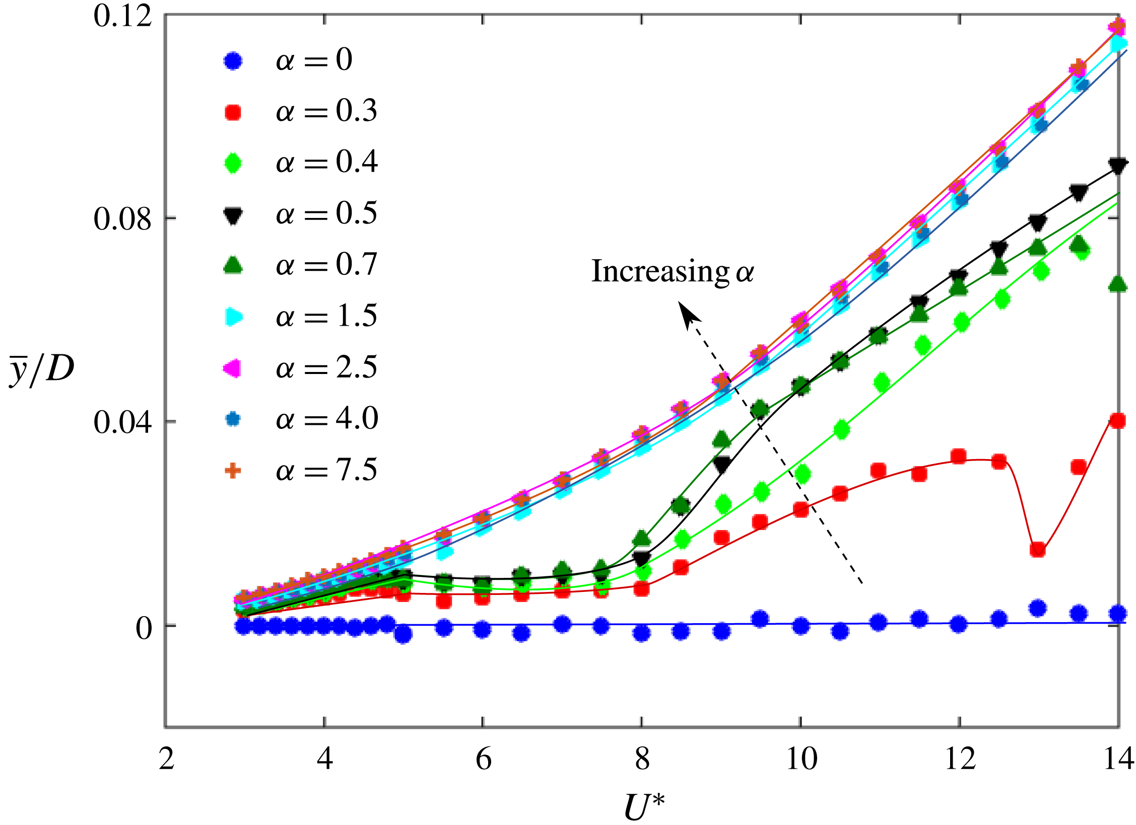
Figure 11. Variation of non-dimensional mean displacement of the sphere ( $\overline{y}/D$ ) with the reduced velocity for different rotation rates. The dashed line arrow represents the direction of increasing $\unicode[STIX]{x1D6FC}$ .

Figure 11 shows the non-dimensional time-averaged displacement of the sphere as a function of reduced velocity for increasing rotation rates. The time-averaged displacement remains around zero for the non-rotating case, but increases with $\unicode[STIX]{x1D6FC}$ . This is due to the rotation-induced Magnus force that exerts a one-sided fluid force acting on the sphere. It can be noted that beyond $\unicode[STIX]{x1D6FC}=1.5$ , there is very slight increase in the time-averaged displacement, suggesting that the magnitude of the Magnus force is limited. Similar behaviour has also been observed in previous studies of rigidly mounted rotating spheres by Macoll (Reference Macoll1928), Barlow & Domanski (Reference Barlow and Domanski2008), Kray et al. (Reference Kray, Franke and Frank2012) and Kim et al. (Reference Kim, Choi, Park and Yoo2014), showing that the increase in the lift coefficient of a sphere reaches a plateau as $\unicode[STIX]{x1D6FC}$ is increased to a certain value, which depends on the Reynolds number.

Figure 12. Frequency response as a function of $U^{\ast }$ correlated with the amplitude response curve (above): (a.i,a.ii) $\unicode[STIX]{x1D6FC}=0$ ; (b.i,b.ii) $\unicode[STIX]{x1D6FC}=1$ . Here, the contour map represents a logarithmic-scale power spectrum depicting the frequency ( $f^{\ast }=f/f_{nw}$ ) content as $U^{\ast }$ is varied. The dashed line represents the value of $f_{vo}$ , which is the vortex shedding frequency of a static sphere.

Figure 12 shows logarithmic-scale power-spectrum plots depicting the dominant oscillation frequency content ( $f^{\ast }=f/f_{nw}$ ) as a function of reduced velocity for both the non-rotating case ( $\unicode[STIX]{x1D6FC}=0$ ) and the rotating case ( $\unicode[STIX]{x1D6FC}=1$ ). The dashed line represents the value of $f_{vo}$ , which is the vortex shedding frequency of a static sphere. Note that the power spectra were computed using fast Fourier transforms (FFTs) of the displacement time series for each $U^{\ast }$ and then normalised by the maximum power. As can be seen in the figure, the dominant oscillation frequency remained close to the natural frequency of the system over the entire lock-in range for the rotating and non-rotating cases. This was found to be true for all $\unicode[STIX]{x1D6FC}$ values investigated.

Figure 13 shows phase-space plots of the measured velocity ( ${\dot{y}}$ ) (normalised by its maximum value) versus (normalised) fluctuating displacement ( ${\tilde{y}}$ ) at $\unicode[STIX]{x1D6FC}=0.5$ for four different $U^{\ast }$ values spanning the range from where the frequency response is near periodic to where it becomes chaotic. Figure 13(a) shows a relatively thin topologically circular structure corresponding to a strongly periodic sphere vibration response. On the other hand, as the sphere goes through the transition from a near periodic to less periodic response, as depicted in figure 13(b,d), the width of the phase-space region covered by successive orbits increases substantially. This is consistent with the frequency contour plots shown previously in figure 12), and the accompanying displacement time traces shown in this figure. Even at $U^{\ast }=9.5$ , where the vibration amplitude has dropped considerably from the peak response, there are signs of intermittency or mode switching, which increase at higher $U^{\ast }$ . For an even higher $U^{\ast }$ value of 14.0, as shown in figure 13(d), where the vibration amplitude is very small, a highly non-periodic response is observed with intermittent bursts of higher-amplitude vibrations located within an otherwise minimal response.

To add further insight to this transition, a variant of the Poincaré surface of section approach was used to further investigate the transition to non-stationary dynamics. These maps are obtained by plotting normalised sphere displacement, $y/D$ , against its value one complete cycle previously. The points are mapped at every upward zero crossing of the sphere transverse velocity for more than 100 vibration cycles. This approach was used to explore the transition to chaos in the wake of a rolling sphere by Rao et al. (Reference Rao, Passaggia, Bolnot, Thompson, Leweke and Hourigan2012) based on numerical simulations, showing the breakdown of periodic orbits through the appearance of Kolmogorov–Arnold–Moser (KAM) tori eventually resulting in a chaotic state as the Reynolds number was further increased. Figure 14 shows such recurrence maps at $\unicode[STIX]{x1D6FC}=0.5$ for four different $U^{\ast }$ values. As is evident from figure 14(a), at $U^{\ast }=6$ , when the vibrations are highly periodic, the points are clustered over a confined region of parameter space consistent with a near-periodic system state. As the $U^{\ast }$ value is increased to higher values of $U^{\ast }=9.5$ and $U^{\ast }=10.5$ , as shown in 14(b) and (c), respectively, the points start to spread in space, mainly along a diagonal line. For $U^{\ast }=14.0$ , the points now appear much more randomly distributed over a larger region. Together with the phase portraits and frequency spectra, this sequence of plots indicates that the system is undergoing a transition to chaotic oscillations.

Figure 13. Phase-space plots for $\unicode[STIX]{x1D6FC}=0.5$ , correlated with the time trace of the fluctuating displacement signal (above each map) at four different reduced velocities: (a) $U^{\ast }=6$ ; (b) $U^{\ast }=9.5$ ; (c) $U^{\ast }=10.5$ ; (d) $U^{\ast }=14.0$ .

Figure 14. Recurrence maps for $y_{o}/D$ , taken for each upward zero crossing of the sphere transverse velocity at $\unicode[STIX]{x1D6FC}=0.5$ for various $U^{\ast }$ values: $U^{\ast }=6$ (a); 9.5 (b); 10.5 (c); 14 (d).

Figure 15. Recurrence plots (lower) of the time series of the normalised body displacement (upper) for $U^{\ast }=6.0$ (a), 9.5 (b), 10.5 (c) and 14.0 (d) at $\unicode[STIX]{x1D6FC}=0.5$ . Note that $\unicode[STIX]{x1D70F}=t/T$ is the normalised time.

To further explore how the vibration response evolves gradually from periodic to chaotic, figure 15 presents corresponding recurrence plots (RPs) based on the body displacement signal for the aforementioned four $U^{\ast }$ values at $\unicode[STIX]{x1D6FC}=0.5$ . Recurrence plots, first designed by Eckmann, Kamphorst & Ruelle (Reference Eckmann, Kamphorst and Ruelle1987) to visually analyse the recurring patterns in time series of dynamical systems, have been utilised in a great variety of scientific areas, from physics (e.g. detection of chaos in nonlinear dynamical systems), to finance and economics, Earth science, biological systems (e.g. in cardiology, neuro-psychology), etc. A historical review of RPs has been given by Marwan (Reference Marwan2008). The construction method for the present RPs is detailed in Marwan et al. (Reference Marwan, Romano, Thiel and Kurths2007). As illustrated in figure 15(a), for the case of $U^{\ast }=6.0$ , where the body vibration is highly periodic, the RP exhibits diagonal oriented periodic checkerboard structures. These structures are symmetric about the main ( $45^{\circ }$ ) diagonal (also known as the line of identity (LOI)). As demonstrated in Marwan (Reference Marwan2003) and Marwan et al. (Reference Marwan, Romano, Thiel and Kurths2007), the diagonal lines parallel to the LOI indicate that the evolution of states of a dynamical system is similar at different epochs, while the diagonal lines orthogonal to the LOI also indicate the evolution of states of a dynamical system is similar at different epochs but with respect to reverse time. It is apparent that these diagonal lines parallel to the LOI are separated by a fixed horizontal distance matching the oscillation period, which is indicative of highly periodic recurrent dynamics with a single dominant frequency. As noted in Marwan et al. (Reference Marwan, Romano, Thiel and Kurths2007), for a quasi-periodic system (as opposed to the current case), the distances between the diagonal lines may vary to form more complex recurrent structures. As the reduced velocity is increased to $U^{\ast }=9.5$ and 10.5 in figures 15(b) and 15(c), respectively, the periodicity of body vibration tends to reduce with less parameter space covered by checkerboard patterns in the RPs. It should also be noted that there is an increasing trend of horizontal (and mirror vertical) curvy lines, which indicate the evolution of states of the system is similar at different epochs but with different rates; in other words, the dynamics of the system could be changing (Marwan et al. Reference Marwan, Romano, Thiel and Kurths2007) (e.g. a non-stationary system with time-varying frequency). As the velocity is further increased to $U^{\ast }=14.0$ in figure 15(d), it becomes difficult to identify any well-defined checkerboard or recurrent structures in the RP. Some horizontal curvy lines and their mirrored counterparts become flatter compared to the cases of $U^{\ast }=9.5$ and 10.5, indicating that some states do not change or change slowly for some time (e.g. for $12<\unicode[STIX]{x1D70F}<17$ ). Additionally, the RP exhibits some single points, indicating that the process may be an uncorrelated random or even anti-correlated (Marwan et al. Reference Marwan, Romano, Thiel and Kurths2007). At this point, it can be concluded that the state of the dynamical system becomes chaotic.

As an alternative depiction of the amplitude responses displayed in figure 7, figure 16 shows a response contour map of the sphere vibration in $U^{\ast }$ – $\unicode[STIX]{x1D6FC}$ parameter space. This clearly shows the shift in high-amplitude response to lower $U^{\ast }$ values as the rotation rate is increased. Even though rotation suppresses large-amplitude oscillation as $\unicode[STIX]{x1D6FC}$ is increased towards unity, there remains a band of moderate oscillation centred at $U^{\ast }\sim 5.5$ that decreases in amplitude much more slowly beyond this $\unicode[STIX]{x1D6FC}$ value. Perhaps also of interest is that high-amplitude oscillation is mainly limited to $\unicode[STIX]{x1D6FC}\lesssim 0.8$ . Previous studies (e.g. Giacobello, Ooi & Balachandar Reference Giacobello, Ooi and Balachandar2009; Kim Reference Kim2009; Poon et al. Reference Poon, Ooi, Giacobello, Iaccarino and Chung2014, and references therein) have shown that the onset of the shear-layer instability wake state of a non-oscillating rotating sphere occurs beyond this $\unicode[STIX]{x1D6FC}$ value. That wake state forms when fluid that passes the retreating side of the sphere is pushed towards the other side of the wake to form a distinctive one-sided separating shear layer, thus changing the characteristic formation and release of vortex loops that defines the non-rotating wake state. The nature of the wake state as a function of rotation rate is examined using flow visualisation and particle image velocimetry in § 5.

Figure 16. The VIV response contour map for a rotating sphere in $U^{\ast }{-}\unicode[STIX]{x1D6FC}$ parameter space. Different contour lines depict different amplitude levels as shown in the figure legend.

4.2 The effective added-mass coefficient and critical mass ratio

Previous studies of VIV of a circular cylinder have shown the existence of a critical mass ratio, $m_{crit}^{\ast }$ , below which large-amplitude body oscillations will persist up to infinite $U^{\ast }$ (Govardhan & Williamson Reference Govardhan and Williamson2002; Jauvtis & Williamson Reference Jauvtis and Williamson2004). The critical mass ratio can be deduced, as given by Govardhan & Williamson (Reference Govardhan and Williamson2002), by evaluating the effective added-mass coefficient $C_{EA}$  in the synchronisation regime. The effective added mass, $m_{EA}=C_{EA}m_{d}$ , is (the negative of) the component of the total force in phase with the acceleration divided by the acceleration. Its significance is that from (3.2) under the condition of low damping, the system frequency depends on the sum of the system mass plus the effective added mass, i.e. $2\unicode[STIX]{x03C0}f=\sqrt{k/(m+m_{EA})}$ , hence if $m\rightarrow -m_{EA}$ , the system response frequency becomes unbounded. Non-dimensionalising this equation and rearranging gives an expression for $C_{EA}$ :

(4.2) $$\begin{eqnarray}C_{EA}=m^{\ast }\left(\frac{1-{f^{\ast }}^{2}}{{f^{\ast }}^{2}}\right)+\left(\frac{C_{A}}{{f^{\ast }}^{2}}\right),\end{eqnarray}$$

in which $C_{A}$  is the potential-flow added-mass coefficient ( $C_{A}=0.5$ for a non-rotating or rotating sphere).

For low mass-damping( $m^{\ast }\text{-}\unicode[STIX]{x1D701}$ ) systems, as proposed by Govardhan & Williamson (Reference Govardhan and Williamson2002), the critical mass ratio can be evaluated by $m_{crit}^{\ast }=\text{max}(-C_{EA})$ . Govardhan & Williamson (Reference Govardhan and Williamson2002) reported $m_{crit}^{\ast }=0.54$ for 1-DOF transverse VIV of a cylinder and $m_{crit}^{\ast }=0.52$ for the 2-DOF case, and $m_{crit}^{\ast }\sim 0.6$ for 2-DOF VIV of a sphere. All these values were reported for very low mass-damping systems ( $m^{\ast }\unicode[STIX]{x1D701}\leqslant 0.04$ ) for moderate Reynolds numbers of $Re\sim 2000$ to $Re\sim 20\,000$ . The mass-damping coefficient here is approximately 0.02.

Figure 17. Effective added mass as a function of $U^{\ast }$ for $\unicode[STIX]{x1D6FC}=0$ (○) and 1 (▫). Data from Govardhan & Williamson (Reference Govardhan and Williamson2005) for low-mass 2-DOF tethered spheres are provided for comparison ( $\times$ , $m^{\ast }=1.31$ ; $+$ , $m^{\ast }=2.83$ ).

Figure 17 shows the variation of $C_{EA}$  with $U^{\ast }$ in the synchronisation range, for the current study with $m^{\ast }=14.2$ , for both the non-rotating case ( $\unicode[STIX]{x1D6FC}=0$ ) and a rotating case ( $\unicode[STIX]{x1D6FC}=1$ ). The coefficient $C_{EA}$  is computed using (4.2), in the same manner as in Govardhan & Williamson (Reference Govardhan and Williamson2002). Results from the current study are directly compared to previously reported $C_{EA}$  data for sphere vibrations with 2-DOF (tethered spheres) for relatively low mass ratios. It can be observed from the figure that $C_{EA}$  for a non-rotating sphere ( $\unicode[STIX]{x1D6FC}=0$ ) with 1-DOF is similar to that of the 2-DOF case. The mass ratio does not seem to significantly affect $C_{EA}$ , at least for this range of $m^{\ast }$ . With imposed rotation, $C_{EA}$  for sphere vibration reduces more quickly with $U^{\ast }$ , following the shift in the response curves with rotation rate, as is evident in figure 17. However, the maximum value of $-C_{EA}$ appears similar.

The maximum of $-C_{EA}$ for the cases shown in figure 17 is ${\sim}0.7$ . Hence, from the above comparison, it can be concluded that the critical mass for both rotating and non-rotating sphere vibration is $m_{crit}^{\ast }\sim 0.7$ . However, there is some scatter in the data, which is consistent with the relatively large mass ratio relative to the critical mass ratio causing the system frequency to depart only slightly from the natural frequency. Thus, the result is not inconsistent with the value of $m_{crit}^{\ast }\simeq 0.6$ proposed by Govardhan & Williamson (Reference Govardhan and Williamson2002) using much lighter spheres. Perhaps what is more interesting is that the non-rotating and rotating values are similar. The result also seems to suggest that the critical mass is not sensitive to the number of degrees of freedom of oscillation, in agreement with the finding for a circular cylinder.

4.3 Effect of rotation on the force coefficients

In this section, the focus is on the effect of transverse rotation on the lift force coefficient for the first two modes within the fundamental synchronisation regime. Results are presented for a selection of rotation rates studied for the same experimental configuration used previously in § 4.1. The dimensionless fluctuating total lift coefficient $C_{y_{rms}}^{\prime }$ , and the total phase ( $\unicode[STIX]{x1D719}_{total}$ ) and the vortex phase ( $\unicode[STIX]{x1D719}_{vortex}$ ) are defined in accordance with the discussion in § 3.2.

Figure 18. Variation of the total phase ( $\unicode[STIX]{x1D719}_{total}$ ) and the vortex phase ( $\unicode[STIX]{x1D719}_{vortex}$ ) with $U^{\ast }$ for $\unicode[STIX]{x1D6FC}=1$ . Measured phase variations (b), correlated with the amplitude response curve (a). The vortex phase starts to rise from low values at the start of Mode I reaching ${\sim}170^{\circ }$ near the peak of Mode II. In contrast, the total phase only begins to rise from ${\sim}0^{\circ }$ as the response reaches close to the peak values in Mode II. (Compare figure 5).

Figure 18 shows the variation of the total phase ( $\unicode[STIX]{x1D719}_{total}$ ) and the vortex phase ( $\unicode[STIX]{x1D719}_{vortex}$ ) with $U^{\ast }$ for $\unicode[STIX]{x1D6FC}=1.0$ . It can be observed that the vortex phase ( $\unicode[STIX]{x1D719}_{vortex}$ ) starts to rise from low values ( ${\sim}30{-}40^{\circ }$ ) at the start of Mode I reaching ${\sim}170^{\circ }$ near the $A_{10}^{\ast }$ peak of Mode II. In contrast, the total phase ( $\unicode[STIX]{x1D719}_{total}$ ) only starts to rise from ${\sim}0^{\circ }$ as the amplitude response reaches close to the peak value in Mode II. These trends were also evident in the non-rotating case shown in figure 5. However, when the vibrations are suppressed, beyond $U^{\ast }=10$ in this case, both $\unicode[STIX]{x1D719}_{total}$ and $\unicode[STIX]{x1D719}_{vortex}$ settle down at approximately $90^{\circ }$ . Similar behaviour was observed for other rotation rates as well.

Figure 19. Variation of the $C_{y_{rms}}^{\prime }$ with reduced velocity for different rotation rates.

Figure 19 shows the r.m.s. of total lift coefficient $C_{y_{rms}}^{\prime }$ versus the reduced velocity for various rotation rates. Note that for $\unicode[STIX]{x1D6FC}=7.5$ the signal-to-noise ratio was poor in the force sensor signals due to negligible response of the sphere, hence the theoretical estimate (as discussed in § 2) has been reported for that case. For the non-rotating case ( $\unicode[STIX]{x1D6FC}=0$ ), there is a sudden jump in $C_{y_{rms}}^{\prime }$ at $U^{\ast }\sim 5$ that is associated with the sudden increase in the amplitude response (lock-in), as shown in figure 7. For increasing $\unicode[STIX]{x1D6FC}$ , the fluctuating force coefficient decreases monotonically and gradually, in accordance with the decreasing amplitude response, as shown in figure 7. The peak value of $C_{y_{rms}}^{\prime }$ also decreases gradually with increasing $\unicode[STIX]{x1D6FC}$ . For $\unicode[STIX]{x1D6FC}=7.5$ , no jump was observed in $C_{y_{rms}}^{\prime }$ , consistent with negligible body oscillations, as shown in figure 7. These observed behaviours of the coefficient $C_{y_{rms}}^{\prime }$ are consistent with the amplitude response. It appears that the imposed transverse rotation decreases the fluctuating component of the lift force, and in turn, that leads to a decrease in the oscillation amplitude.

Figure 20. Time trace of the total lift coefficient, $C_{y}$ (b), correlated with the displacement signal (a) for $\unicode[STIX]{x1D6FC}=0.7$ at $U^{\ast }=6$ . Asymmetry in the force signal as the sphere traverses from the advancing to the retreating side is evident in the time trace.

Figure 20(b) shows the time trace of the total lift force coefficient, $C_{y}$ , for rotation rate $\unicode[STIX]{x1D6FC}=0.7$ , at a reduced velocity of $U^{\ast }=6$ , correlated with the sphere displacement (shown in figure 20 a). As apparent from the figure, there is an evident asymmetry in the force signal as the sphere traverses from the advancing side to the retreating side. This is indicative of the differences in the wake shedding pattern from one half-cycle to the next as the sphere moves from one side to the other. This will be examined further in § 5.

4.3.1 Competition between the Magnus force and the fluctuating lift force

The imposed rotation decreases the fluctuating component of the transverse force that drives the oscillations of the sphere. It also increases the mean component of the transverse force due to the Magnus effect. Hence, in order to better understand the dynamics of this problem, the total transverse force coefficient acting on the sphere can be split into two components, as $C_{y}=\overline{C}_{y}+C_{y_{rms}}^{\prime }$ , where $\overline{C}_{y}$ is the time-averaged mean transverse force coefficient and $C_{y_{rms}}^{\prime }$ is the fluctuating transverse force coefficient. Under resonance, where the assumption is often made that ( $U^{\ast }/f^{\ast }$ ) and $f^{\ast }$ are constant, $A^{\ast }$ is directly correlated to $C_{y}$ for a fixed mass-damping system by

(4.3) $$\begin{eqnarray}A^{\ast }\propto \frac{C_{y}^{\prime }\sin \unicode[STIX]{x1D719}}{(m_{A}+C_{A})\unicode[STIX]{x1D701}},\end{eqnarray}$$

where $\unicode[STIX]{x1D719}$ is the phase difference between the body displacement and transverse force. This can be derived from (2.1), (3.2) and (3.1), as also shown by Williamson & Govardhan (Reference Williamson and Govardhan2004). Also, the non-dimensionalised mean displacement of the sphere, $\overline{y}/DU^{\ast 2}$ , is directly correlated to the mean transverse force coefficient $\overline{C}_{y}$ by

(4.4) $$\begin{eqnarray}\frac{\overline{y}}{DU^{\ast 2}}=\frac{\overline{C}_{y}}{2\unicode[STIX]{x03C0}^{3}(C_{A}+m^{\ast })}.\end{eqnarray}$$

Initially, for the non-rotating sphere undergoing VIV, $\overline{C}_{y}$ is zero and $C_{y_{rms}}^{\prime }$ drives the oscillations. As $\unicode[STIX]{x1D6FC}$ is increased, the component of $\overline{C}_{y}$ increases and the r.m.s. value of the fluctuating component $C_{y_{rms}}^{\prime }$ decreases. For lower rotation rates, the Magnus effect is not very strong, so there seems to be a competition between the increasing Magnus force and the competing fluctuating transverse force. Such a competition is evident for only lower rotation rates in the current study.

Figure 21. Comparison of the response characteristics for $\unicode[STIX]{x1D6FC}=0.4$ (a–d) and $\unicode[STIX]{x1D6FC}=2.5$ (e–h). The quantity plotted in each row is shown at the left.

In the left column, figure 21(a–d) shows that the fluctuating oscillation amplitude, $A^{\ast }$ , is closely correlated with the fluctuating transverse force coefficient, $C_{y_{rms}}^{\prime }$ , and the non-dimensionalised mean displacement amplitude, $\overline{y}/DU^{\ast 2}$ , directly correlates with the mean transverse force coefficient, $\overline{C}_{y}$ , for $\unicode[STIX]{x1D6FC}=0.4$ . The right column of figure 21(e–h) shows the same plots for $\unicode[STIX]{x1D6FC}=2.5$ . These variations confirm the theoretical relationships given by the two equations above. The response for $\unicode[STIX]{x1D6FC}=0.4$ can be broadly divided into three regimes for this case. In region I, ${C_{y}}_{rms}^{\prime }$ is large due to the resonance between the vortex shedding and body oscillation frequencies covering Mode I and the Mode II peak. For this region, $\overline{C}_{y}$ is reduced with a concomitant effect in $\overline{y}/DU^{\ast 2}$ . In region II, which corresponds to the plateau response range after the Mode II peak, the fluctuating forcing is less and the mean force increases, leading to increased mean displacement offset. The competition between the two force components is clearly evident. In region III, the Magnus effect dominates, with $\overline{C}_{y}$ again reaching a constant value close to that at low $U^{\ast }$ before lock-in. Simultaneously, there is sudden drop in the $A^{\ast }$ and ${C_{y}}_{rms}^{\prime }$ in the desynchronisation regime at high $U^{\ast }$ .

The sudden rebound in the amplitude response observed for a rotation rate of $\unicode[STIX]{x1D6FC}=0.3$ at higher $U^{\ast }$ values of ${\sim}16{-}17$ (see figure 7) can also be explained on such grounds. A brief study by Sareen et al. (Reference Sareen, Zhao, Lo Jacono, Sheridan, Hourigan and Thompson2016) investigated the effect of rotation on the force coefficients of a fixed rotating sphere by measuring the drag and lift coefficient for varying rotation rates ( $0\leqslant \unicode[STIX]{x1D6FC}\leqslant 6$ ) at several Reynolds numbers. They observed a sudden drop in the lift coefficient at $\unicode[STIX]{x1D6FC}=0.3$ for a Reynolds number of $Re=2.75\times 10^{4}$ . Interestingly, the Reynolds number where the sudden rebound is observed in the current study varies between $2.75\times 10^{4}$ and $2.9\times 10^{4}$ corresponding to the $U^{\ast }$ range 16–17. Thus, it can be conjectured that here also there is a sudden drop in the mean lift force acting on the sphere at $\unicode[STIX]{x1D6FC}=0.3$ for $U^{\ast }\sim 16{-}17$ . In lieu of the competition between the mean lift force and the fluctuating force, the fluctuating force is allowed to suddenly increase leading to a sudden rebound in the amplitude response.

However, at higher rotation rates, for example at $\unicode[STIX]{x1D6FC}=2.5$ as shown in figure 21, the Magnus force dominates over the entire $U^{\ast }$ range, even though there is a narrow resonant regime. This leads to almost constant values of $\overline{y}/DU^{\ast ^{2}}$ and $\overline{C}_{y}$ . For this case, $A^{\ast }$ and ${C_{y}}_{rms}^{\prime }$ remain at low values over the entire $U^{\ast }$ range. How the sphere rotation affects vortex shedding and thereby leads to the attenuation of VIV will be discussed in § 5.