2.1 Model formulation

The flow considered is that of an incompressible fluid in a rectangular domain with dimensions $(L_{x},L_{y},L_{z})$ , where $x$ , $y$ , $z$ or $x_{1}$ , $x_{2}$ , $x_{3}$ represent the streamwise, wall-normal and spanwise coordinates, respectively. The corresponding velocity components are denoted by $u$ , $v$ , $w$ or $u_{1}$ , $u_{2}$ , $u_{3}$ and time is denoted by $t$ . A solid wall is located at the lower boundary of the domain at $y=0$ . Given the kinematic viscosity $\unicode[STIX]{x1D708}$ and the fluid density $\unicode[STIX]{x1D70C}$ , the instantaneous wall shear stress is defined as

(2.1) $$\begin{eqnarray}\displaystyle \unicode[STIX]{x1D70F}_{w}(t)=\unicode[STIX]{x1D70C}\unicode[STIX]{x1D708}\left\langle \left.{\displaystyle \frac{\unicode[STIX]{x2202}u}{\unicode[STIX]{x2202}y}}\right|_{y=0}\right\rangle _{x,z}, & & \displaystyle\end{eqnarray}$$

where $\langle ~\cdot ~\rangle _{x,z}$ denotes the average in the streamwise and spanwise directions. The wall shear stress of the ‘turbulent state’, $\overline{\unicode[STIX]{x1D70F}_{w}}$ , is subsequently obtained from a full simulation, where $\overline{~\cdot ~}$ denotes the average in time while the flow remains turbulent. The reference friction velocity is defined as $u_{\unicode[STIX]{x1D70F},r}=\sqrt{\overline{\unicode[STIX]{x1D70F}_{w}}/\unicode[STIX]{x1D70C}}$ and the viscous length scale is then defined as $\unicode[STIX]{x1D6FF}_{\unicode[STIX]{x1D708}}=\unicode[STIX]{x1D708}/u_{\unicode[STIX]{x1D70F},r}$ . Using $\unicode[STIX]{x1D6FF}_{\unicode[STIX]{x1D708}}$ as the characteristic length scale and $u_{\unicode[STIX]{x1D70F},r}$ as the characteristic velocity scale, the model is formulated in inner units with the velocity field $\boldsymbol{u}^{+}=(u^{+},v^{+},w^{+})=(u,v,w)/u_{\unicode[STIX]{x1D70F},r}$ , spatial coordinates $\boldsymbol{x}^{+}=(x^{+},y^{+},z^{+})=(x,y,z)/\unicode[STIX]{x1D6FF}_{\unicode[STIX]{x1D708}}$ and time $t^{+}=tu_{\unicode[STIX]{x1D70F},r}^{2}/\unicode[STIX]{x1D708}$ . A diagram of the flow geometry is shown in figure 1.

Figure 1. Flow geometry of the shear stress-driven model.

Employing the Reynolds decomposition, the velocity field can be expressed in terms of the mean and fluctuating components

(2.2) $$\begin{eqnarray}\displaystyle \boldsymbol{u}^{+}(\boldsymbol{x}^{+},t^{+})=\boldsymbol{U}^{+}(y^{+})+\boldsymbol{u}^{^{\prime }+}(\boldsymbol{x}^{+},t^{+}), & & \displaystyle\end{eqnarray}$$

where $\boldsymbol{U}^{+}(y^{+})=(U^{+}(y^{+}),0,0)=(\overline{\langle u^{+}\rangle }_{x^{+},z^{+}},0,0)$ and $\boldsymbol{u}^{^{\prime }+}=(u^{^{\prime }+},v^{^{\prime }+},w^{^{\prime }+})$ . In channel flows, the turbulent mean and fluctuating velocity components satisfy the equations

(2.3) $$\begin{eqnarray}\displaystyle {\displaystyle \frac{\text{d}U^{+}}{\text{d}y^{+}}}-\overline{\langle u^{^{\prime }+}v^{^{\prime }+}\rangle }_{x^{+},z^{+}}=1-{\displaystyle \frac{y^{+}}{Re_{\unicode[STIX]{x1D70F}}}}, & & \displaystyle\end{eqnarray}$$

(2.4) $$\begin{eqnarray}\displaystyle \boldsymbol{u}_{t^{+}}^{^{\prime }+}+(\boldsymbol{U}^{+}\boldsymbol{\cdot }\unicode[STIX]{x1D735})\boldsymbol{u}^{^{\prime }+}+(\boldsymbol{u}^{^{\prime }+}\boldsymbol{\cdot }\unicode[STIX]{x1D735})\boldsymbol{U}^{+} & = & \displaystyle -\unicode[STIX]{x1D735}p^{^{\prime }+}+\unicode[STIX]{x1D6FB}^{2}\boldsymbol{u}^{^{\prime }+}-(\boldsymbol{u}^{^{\prime }+}\boldsymbol{\cdot }\unicode[STIX]{x1D735})\boldsymbol{u}^{^{\prime }+}\nonumber\\ \displaystyle & & \displaystyle +\,\overline{\langle (\boldsymbol{u}^{^{\prime }+}\boldsymbol{\cdot }\unicode[STIX]{x1D735})\boldsymbol{u}^{^{\prime }+}\rangle }_{x^{+},z^{+}},\end{eqnarray}$$

where $p^{^{\prime }+}$ is the pressure fluctuation and the $-y^{+}/Re_{\unicode[STIX]{x1D70F}}$ term is derived from the imposed pressure gradient (e.g. Townsend Reference Townsend1980). Within the mesolayer, the wall-normal coordinate satisfies the relation $y^{+}\sim \sqrt{Re_{\unicode[STIX]{x1D70F}}}$ (Sreenivasan & Sahay Reference Sreenivasan, Sahay and Panton1997; Wei et al. Reference Wei, Fife, Klewicki and McMurtry2005). Therefore, as $Re_{\unicode[STIX]{x1D70F}}\rightarrow \infty$ , the $-y^{+}/Re_{\unicode[STIX]{x1D70F}}$ term will vanish provided that $L_{y}^{+}\sim \sqrt{Re_{\unicode[STIX]{x1D70F}}}$ . For parallel wall-bounded flows more generally, any terms in the mean momentum equation that are associated with the given flow geometry must vanish in the limit of $Re_{\unicode[STIX]{x1D70F}}\rightarrow \infty$ . The model is then governed by the following momentum equations for the turbulent mean and fluctuating components,

(2.5) $$\begin{eqnarray}\displaystyle {\displaystyle \frac{\text{d}U^{+}}{\text{d}y^{+}}}-\overline{\langle u^{^{\prime }+}v^{^{\prime }+}\rangle }_{x^{+},z^{+}}=1, & & \displaystyle\end{eqnarray}$$

(2.6) $$\begin{eqnarray}\displaystyle \boldsymbol{u}_{t^{+}}^{^{\prime }+}+(\boldsymbol{U}^{+}\boldsymbol{\cdot }\unicode[STIX]{x1D735})\boldsymbol{u}^{^{\prime }+}+(\boldsymbol{u}^{^{\prime }+}\boldsymbol{\cdot }\unicode[STIX]{x1D735})\boldsymbol{U}^{+} & = & \displaystyle -\unicode[STIX]{x1D735}p^{^{\prime }+}+\unicode[STIX]{x1D6FB}^{2}\boldsymbol{u}^{^{\prime }+}-(\boldsymbol{u}^{^{\prime }+}\boldsymbol{\cdot }\unicode[STIX]{x1D735})\boldsymbol{u}^{^{\prime }+}\nonumber\\ \displaystyle & & \displaystyle +\,\overline{\langle (\boldsymbol{u}^{^{\prime }+}\boldsymbol{\cdot }\unicode[STIX]{x1D735})\boldsymbol{u}^{^{\prime }+}\rangle }_{x^{+},z^{+}}.\end{eqnarray}$$

At the lower boundary of the domain, a no-slip condition is imposed to represent the stationary wall,

(2.7) $$\begin{eqnarray}\displaystyle \boldsymbol{u}^{+}|_{y^{+}=0}=\mathbf{0}, & & \displaystyle\end{eqnarray}$$

whereas at the upper boundary, a horizontally uniform shear stress is applied. The uniform shear stress condition at the upper boundary is implemented such that the bulk flow rate across the domain is maintained during simulations. For this purpose, the instantaneous bulk velocity is defined as $U_{b}^{+}(t^{+})=\langle u^{+}(x^{+},y^{+},z^{+},t^{+})\rangle _{x^{+},y^{+},z^{+}}$ ( $\langle \cdot \rangle _{x^{+},y^{+},z^{+}}$ denotes the volume average) and the laminar bulk velocity is denoted by $U_{0}^{+}$ . Then, the streamwise boundary condition is expressed as

(2.8) $$\begin{eqnarray}\displaystyle \left.{\displaystyle \frac{\unicode[STIX]{x2202}u^{+}}{\unicode[STIX]{x2202}y^{+}}}\right|_{y^{+}=L_{y}^{+}}(t^{+})=\left.\left\langle {\displaystyle \frac{\unicode[STIX]{x2202}u^{+}}{\unicode[STIX]{x2202}y^{+}}}\right|_{y^{+}=0}\right\rangle _{x^{+},z^{+}}(t^{+})+C^{+}(U_{0}^{+}-U_{b}^{+}(t^{+})), & & \displaystyle\end{eqnarray}$$

where $C^{+}$ is a tuning constant that maintains $U_{b}^{+}(t^{+})$ close to $U_{0}^{+}$ during simulations. Given that the fluctuation of $U_{b}^{+}(t^{+})$ about $U_{0}^{+}$ is kept to a minimum, the flow is largely independent of the value of $C^{+}$ but $C^{+}\approx 0.28$ is the value used throughout the present study. Since $\overline{U_{b}^{+}(t^{+})}=U_{0}^{+}$ , equation (2.8) implies that the time-averaged total shear stress (i.e. the sum of molecular and Reynolds stresses) is uniform across the entire domain as long as the wall-normal velocity at the upper boundary is zero, ensuring that the mean momentum equation (2.5) is satisfied. During the simulations of the present study, $U_{0}^{+}-U_{b}^{+}(t^{+})$ has indeed been found to be very small, indicating that only a very small amount of compensation at the upper boundary is required at each time step to maintain $U_{b}^{+}(t^{+})$ close to $U_{0}^{+}$ . This technique is very similar to that used to maintain constant mass flux in pressure-driven channel flow. At the upper boundary of the domain, impermeability and stress-free conditions are imposed for the wall-normal and spanwise velocity components respectively, namely

(2.9a,b ) $$\begin{eqnarray}\displaystyle v^{+}|_{y^{+}=L_{y}^{+}}=0,\quad \text{and}\quad \left.{\displaystyle \frac{\unicode[STIX]{x2202}w^{+}}{\unicode[STIX]{x2202}y^{+}}}\right|_{y^{+}=L_{y}^{+}}=0, & & \displaystyle\end{eqnarray}$$

ensuring zero Reynolds stress at the upper boundary. The upper boundary conditions of the model may be considered ad hoc, however, such conditions are required to ensure that the structures of the logarithmic and wake layers are safely removed. Periodic boundary conditions are imposed in both the streamwise and spanwise directions. The numerical simulations in this work were performed with the diablo Navier–Stokes solver (Bewley Reference Bewley2014). This code uses spectral methods with a $2/3$ dealiasing rule in the streamwise & spanwise directions and a second-order finite difference scheme in the wall-normal direction, which has been verified extensively (e.g. Hwang Reference Hwang2013).

Several notable features of the present model must also be mentioned. Firstly, equation (2.6) does not seem to contain any explicit control parameter, such as a Reynolds number. This is essentially because the equations of motion are normalised by the viscous length scale $\unicode[STIX]{x1D6FF}_{\unicode[STIX]{x1D708}}$ and reference friction velocity $u_{\unicode[STIX]{x1D70F},r}$ . Under this rescaling, the velocity field is governed by the unit Reynolds number Navier–Stokes equations (2.6). The inner-scaled flow variables are $O(1)$ quantities even in the limit of $Re_{\unicode[STIX]{x1D70F}}\rightarrow \infty$ . However, this does not imply that the equations do not have a control parameter. In this case, the domain dimensions (i.e. $(L_{x}^{+},L_{y}^{+},L_{z}^{+})$ ) are the main control parameters, as long as they are finite. In particular, the spanwise width of the domain can be used to determine the expected multiplicity (or levels in the hierarchy) of integral length scales. For example, if $L_{z}^{+}\simeq 100$ , it will only include the near-wall energy-containing structures at a single integral length scale (Jiménez & Moin Reference Jiménez and Moin1991). If $L_{z}^{+}\simeq 200$ , it will include two integral length scales (i.e. $\unicode[STIX]{x1D706}_{z}^{+}\simeq 100,200$ ) due to the spanwise periodic boundary condition. Secondly, it must be emphasised that (2.5) only governs the turbulent mean velocity field. The laminar state (and other invariant solutions) satisfy

(2.10) $$\begin{eqnarray}\displaystyle {\displaystyle \frac{\text{d}U^{+}}{\text{d}y^{+}}}-\overline{\langle u^{^{\prime }+}v^{^{\prime }+}\rangle }_{x^{+},z^{+}}=\unicode[STIX]{x1D6E5}^{+}, & & \displaystyle\end{eqnarray}$$

where $\unicode[STIX]{x1D6E5}^{+}=\text{d}U^{+}/\text{d}y^{+}|_{y^{+}=0}$ is the wall shear rate of the corresponding solution, which is smaller than unity in the laminar case. However, the present model ensures that the base flow is a uniform shear flow – this can be easily checked by setting the Reynolds stress in (2.10) to zero, with solution $U^{+}=\unicode[STIX]{x1D6E5}^{+}y^{+}$ . The laminar bulk velocity is then 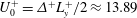$U_{0}^{+}=\unicode[STIX]{x1D6E5}^{+}L_{y}^{+}/2\approx 13.89$ . This implies that the model would be valid in the region close to the wall, where the base flow can be approximated by a uniform shear flow. This also indicates that the base flow in the mesolayer is a uniform shear flow, explaining why the description by (2.5) and (2.6) would be universal for any parallel wall-bounded shear flow. Finally, it is evident that the crucial issue in the use of the present model is the use of the upper boundary condition (2.8), which could potentially affect the region that is to be studied. For this reason, the model is first carefully validated in § 2.2.

2.2 Validation of the shear stress-driven flow model

The shear stress-driven flow model presented in the previous subsection must now be evaluated, and the velocity statistics and spectra compared to that of independent near-wall turbulence. The obvious benchmark for the model is near-wall Couette flow, which exactly satisfies (2.5) and (2.6) at all Reynolds numbers. In order to isolate the near-wall flow, a damping function is introduced to the system, which quashes turbulent fluctuations above a fixed wall-normal height. The damping function employed is

(2.11) $$\begin{eqnarray}\displaystyle \unicode[STIX]{x1D707}^{+}(y^{+})={\displaystyle \frac{\unicode[STIX]{x1D707}_{0}^{+}}{2}}\left[1+\tanh \left(10\left(\left({\displaystyle \frac{y^{+}}{y_{0}^{+}}}\right)^{2}-1\right)\right)\right], & & \displaystyle\end{eqnarray}$$

similar to that used by Jiménez & Pinelli (Reference Jiménez and Pinelli1999). Here, $\unicode[STIX]{x1D707}_{0}^{+}$ denotes the damping amplitude and $y_{0}^{+}$ denotes the damping height, such that $\unicode[STIX]{x1D707}^{+}(y^{+})$ tends to the constant $\unicode[STIX]{x1D707}_{0}^{+}$ above $y_{0}^{+}$ and decays rapidly to zero below this point. Above the damping height, the turbulent fluctuations are damped onto the mean flow, hence the system is governed by the equations

(2.12) $$\begin{eqnarray}\displaystyle \boldsymbol{u}_{t^{+}}^{+}+(\boldsymbol{u}^{+}\boldsymbol{\cdot }\unicode[STIX]{x1D735})\boldsymbol{u}^{+}=-\unicode[STIX]{x1D735}p^{+}+\unicode[STIX]{x1D6FB}^{2}\boldsymbol{u}^{+}-\unicode[STIX]{x1D707}^{+}(y^{+})(\boldsymbol{u}^{+}-\langle \boldsymbol{u}^{+}\rangle _{x^{+},z^{+}}). & & \displaystyle\end{eqnarray}$$

The value of the damping height is chosen to be $y_{0}^{+}\approx 95$ so that the near-wall flow is unaffected. The value of the damping amplitude must be sufficiently high to kill all turbulent fluctuations above the damping height and it was found that $\unicode[STIX]{x1D707}_{0}^{+}\approx 0.33$ achieves appropriate results. Since the damping function kills Reynolds stresses above the damping height, the kinematic viscosity must increase in line with the Fukagata–Iwamoto–Kasagi identity (Fukagata, Iwamoto & Kasagi Reference Fukagata, Iwamoto and Kasagi2002) to maintain similar inner-scaled domain dimensions. To compare both flow configurations, a long streamwise domain length of $L_{x}^{+}\approx 3000$ is chosen so that the longest streaky structures are resolved. However, the spanwise domain width is chosen to be close to that of the minimal unit, $L_{z}^{+}\approx 110$ , so as to remove the wider structures of the outer flow. The shear stress-driven flow model is denoted by SSDF and damped Couette flow by DCF, and the simulation parameters are displayed in table 1. All statistics presented here were computed over a time period of $T^{+}>35\,000$ .

Figure 2. Mean streamwise velocity, $U^{+}(y^{+})$ , of the shear stress-driven flow model (red dashed line), plotted against that of damped Couette flow (black solid line).

Figure 3. Root mean squared velocity of the shear stress-driven flow model; (a) $u_{rms}^{+}$ (red dashed line), (b) $v_{rms}^{+}$ (green solid line) and (c) $w_{rms}^{+}$ (blue dash-dotted line), plotted against that of damped Couette flow (black solid lines).

Table 1. Simulation parameters of the shear stress-driven flow model and damped Couette flow.

Figure 4. Premultiplied one-dimensional streamwise (a,c,e,g) and spanwise (b,d,f,h) wavenumber spectra of the shear stress-driven flow model; (a,b) streamwise velocity, (c,d) wall-normal velocity, (e,f) spanwise velocity and (g,h) Reynolds stress. Isocontours of damped Couette flow are superimposed in black.

The mean streamwise velocity profile of the shear stress-driven flow model compared to that of damped Couette flow is shown in figure 2. There is excellent agreement between the two flow configurations for $y^{+}<70$ but the shear stress-driven model slightly overestimates the mean velocity above this point. The viscous sublayer features the characteristic linear profile, which is also seen near the upper boundary of the domain. Similar behaviour is observed in the root mean squared velocity statistics in figure 3. The shear stress-driven model clearly captures the near-wall peak of the streamwise velocity fluctuation at $y^{+}\approx 12$ but again overestimates the streamwise velocity near the upper boundary. In contrast, the wall-normal and spanwise velocity fluctuations are underestimated by the shear stress-driven model near the upper boundary but show excellent agreement closer to the wall. The premultiplied one-dimensional streamwise and spanwise wavenumber spectra are shown in figure 4. As seen in the first- and second-order statistics, there is excellent agreement between the shear stress-driven model and damped Couette flow for $y^{+}<40$ . The streamwise wavenumber spectra of the streamwise velocity shows slight excitation at longer streamwise wavelengths near the upper boundary, consonant with the previous statistical results. The spectra of the wall-normal and spanwise velocity components are also underestimated near the upper boundary. In general, the spanwise wavenumber spectra of the three velocity components and Reynolds stress show excellent agreement.

3.1 Edge and invariant solutions

As in the case of Couette flow, the base flow of the shear stress-driven flow model has a linear velocity profile. However, any perturbations to the base flow are subject to different boundary conditions than those of Couette flow, namely (2.8) and (2.9), hence the linear stability of the base flow is not guaranteed. A simple way to verify the linear stability of the base flow for the parameters chosen is to determine whether it is possible to compute the edge, the hyper-dimensional manifold that separates initial conditions that relaminarise from those that become fully turbulent (Skufca et al. Reference Skufca, Yorke and Eckhardt2006). In this case, the edge of $\unicode[STIX]{x1D6FA}$ is computed via bisection, in which the turbulent fluctuations of a random initial condition are rescaled so as to lie between specific laminar and turbulent thresholds. This modified velocity field is advanced in time until the transient behaviour has decayed sufficiently, denoted by time $t_{0}^{+}$ . The edge is a fundamental feature of the state space of a parallel wall-bounded shear flow. The turbulent state space is also structured by invariant solutions, including relative equilibrium solutions and relative periodic orbits, whose stable and unstable manifolds guide nearby turbulent trajectories. Such invariant solutions are computed using the Newton–Krylov–Hookstep algorithm (Viswanath Reference Viswanath2007, Reference Viswanath2009; Willis, Cvitanović & Avila Reference Willis, Cvitanović and Avila2013), which has been verified extensively in Hwang et al. (Reference Hwang, Willis and Cossu2016). Given an initial condition $\boldsymbol{u}_{0}^{+}$ , this algorithm seeks to minimise the relative error between the initial condition and its translated time-forward map

(3.2) $$\begin{eqnarray}\displaystyle r={\displaystyle \frac{||\boldsymbol{u}_{0}^{+}-\unicode[STIX]{x1D70F}(s_{x^{+}},s_{z^{+}})f^{T^{+}}(\boldsymbol{u}_{0}^{+})||}{||\boldsymbol{u}_{0}^{+}||}}, & & \displaystyle\end{eqnarray}$$

where $f$ denotes the Navier–Stokes propagator and $\unicode[STIX]{x1D70F}$ represents a translation of distance $s_{x^{+}}$ in the streamwise direction and $s_{z^{+}}$ in the spanwise direction. For periodic orbits, the value of $T^{+}$ is updated at each Newton iteration from a good initial guess and the converged value becomes the time period (up to positive integer multiplication of the fundamental period). For equilibria, the choice of $T^{+}$ is arbitrary but $T^{+}\approx 16$ is the value used for those computed here. All invariant solutions reported in this work satisfy $r<10^{-8}$ . The eigenvalues of converged solutions are subsequently computed via Arnoldi iteration.

Figure 5. The edge of the reference domain $\unicode[STIX]{x1D6FA}$ (black solid line), separating initial conditions that relaminarise (blue dash-dotted lines) from those that become fully turbulent (red dash-dotted lines). $E_{u}^{+}$ is the streamwise turbulent fluctuation energy and $t_{0}^{+}$ is the time by which the initial transient behaviour of the edge has decayed sufficiently. The inset shows the relative periodic orbit embedded in the edge.

Table 3. Properties of the invariant solutions in $\unicode[STIX]{x1D6FA}$ : $T^{+}$ , the time period; $c_{x}^{+}$ , the phase speed; $\unicode[STIX]{x1D6E5}^{+}$ , the wall shear rate; $I/I_{l}$ , the energy input normalised by that of the laminar state; $E_{p}$ , the kinetic energy deviation from the laminar state; $\dim (W^{u})$ , the dimension of the unstable manifold. The $c_{x}^{+}$ , $\unicode[STIX]{x1D6E5}^{+}$ , $I/I_{l}$ and $E_{p}$ values of $PO_{A0L}$ and $PO_{C0U}$ are averages over the period $T^{+}$ .

Defining the streamwise turbulent fluctuation energy as

(3.3) $$\begin{eqnarray}\displaystyle E_{u}^{+}={\textstyle \frac{1}{2}}\langle ({u^{\prime }}^{+})^{2}\rangle _{x^{+},y^{+},z^{+}}, & & \displaystyle\end{eqnarray}$$

the edge of $\unicode[STIX]{x1D6FA}$ as a function of time is shown in figure 5. After the transient behaviour has decayed, the edge initially shows statistically stationary behaviour, from which the first relative equilibrium solution, $EQ_{A1L}$ , was computed. However, this equilibrium solution is unstable to a gentle relative periodic orbit on the edge. In figure 5, the edge trajectory leaves the neighbourhood of the equilibrium solution and is pulled towards the periodic orbit, stabilising at later time. This periodic orbit, titled $PO_{A0L}$ , is stable on the edge and hence it is the edge state. Therefore, the transient visit of $EQ_{A1L}$ in figure 5 is a peculiarity of the initial condition for the bisection, since any edge trajectory in the neighbourhood of $PO_{A0L}$ will approach it monotonically. The other invariant solutions were computed using initial conditions taken directly from the turbulent trajectory or via continuation. In total, two relative periodic orbits and thirteen relative equilibrium solutions were found in $\unicode[STIX]{x1D6FA}$ . They are distinguished into three distinct groups (A, B and C) in the following discussion and their properties are summarised in table 3.

Figure 6. Velocity field visualisation and root mean squared velocity profiles of the Group A relative periodic orbit and relative equilibrium solutions, henceforth titled $PO_{A0L}$ , $EQ_{A1L}$ , $EQ_{A2}$ , $EQ_{A3L}$ and $EQ_{A4L}$ , respectively. The red and blue surfaces represent high- and low-speed streaks; (a,b,d) $u^{+}-\langle u^{+}\rangle _{x^{+},z^{+}}=\pm 3$ , (c,e) $u^{+}-\langle u^{+}\rangle _{x^{+},z^{+}}=\pm 1.5$ . The yellow and green surfaces are iso-surfaces of wall-normal velocity; $v^{+}=\pm 0.12$ . Red dashed lines, $u_{rms}^{+}$ ; green solid lines, $v_{rms}^{+}$ ; blue dash-dotted lines, $w_{rms}^{+}$ . The root mean squared velocity profile of $PO_{A0L}$ is an average over the period $T^{+}$ .

The Group A solutions are characterised by small cross-streamwise velocity fluctuations relative to the streamwise velocity fluctuations. Velocity isosurfaces and second-order statistics are shown in figure 6. Titled $PO_{A0L}$ , $EQ_{A1L}$ , $EQ_{A2}$ , $EQ_{A3L}$ and $EQ_{A4L}$ respectively, each solution in this group is a lower branch solution (figure 9). As previously mentioned, $\mathbf{PO}_{\mathbf{A0L}}$ is the edge state. It is time periodic with $T^{+}\approx 26.2$ , an order of magnitude shorter than the bursting period of near-wall turbulence (Hamilton et al. Reference Hamilton, Kim and Waleffe1995; Jiménez et al. Reference Jiménez, Kawahara, Simens, Nagata and Shiba2005), and its oscillation amplitude is very small ( $t^{+}-t_{0}^{+}\simeq 20\,000$ in figure 5). However, its $E_{u}^{+}$ value is significantly different to that of $EQ_{A1L}$ ( $t^{+}-t_{0}^{+}\simeq 0$ in figure 5), which is noticeable in the $u_{rms}^{+}$ profile near the upper boundary. This periodic orbit might be related to that identified in the near-wall region of Poiseuille flow by Jiménez & Simens (Reference Jiménez and Simens2001) or to the ‘gentle’ periodic orbit on the edge in Kawahara & Kida (Reference Kawahara and Kida2001) (see also Lustro et al. Reference Lustro, Kawahara, van Veen, Shimizu and Kokubu2019). The $\mathbf{EQ}_{\mathbf{A1L}}$ state is the equilibrium solution embedded in the edge. However, it has a three-dimensional unstable manifold; one dimension representing the instability of the edge and the other two representing its instability to $PO_{A0L}$ . It is dominated by a pair of strong streaks, flanked by weaker vortical motion. Examination of the velocity field indicates that this is presumably the stress-driven analogue of Nagata’s lower branch solution (Nagata Reference Nagata1990), without the shift-rotational symmetry possessed by Couette flow. If an appropriate computational domain is provided, Nagata’s lower branch solution also arises as the edge state of Couette flow (Schneider et al. Reference Schneider, Gibson, Lagha, De Lillo and Eckhardt2008). The Group A solutions all have wall shear rates well below the turbulent mean but $\mathbf{EQ}_{\mathbf{A2}}$ is the equilibrium solution with the lowest drag in $\unicode[STIX]{x1D6FA}$ (table 3). In fact, it is analogous to $EQ_{7}$ computed by Gibson, Halcrow & Cvitanovi (Reference Gibson, Halcrow and Cvitanović2009) and is the only solution to comprise of two pairs of streaks. The $\mathbf{EQ}_{\mathbf{A3L}}$ state is a ‘wall-attached’ solution, showing clear vertical localisation and little activity near the upper boundary. It too consists of a pair of strong streaks, driven by cross-streamwise motion an order of magnitude lower. The $\mathbf{EQ}_{\mathbf{A4L}}$ state is the last Group A solution and also exhibits vertical localisation, this time in the domain centre. The maximum streak value is similar to that of $EQ_{A2}$ , hence it has the second-lowest drag in $\unicode[STIX]{x1D6FA}$ . Again, this solution possesses a Couette flow analogue, namely $EQ_{3}$ computed by Gibson et al. (Reference Gibson, Halcrow and Cvitanović2009).

Figure 7. Velocity field visualisation and root mean squared velocity profiles of the Group B relative equilibrium solutions, henceforth titled $EQ_{B5L}$ , $EQ_{B3U}$ , $EQ_{B4U}$ , $EQ_{B6L}$ and $EQ_{B6U}$ , respectively. The red and blue surfaces represent high and low speed streaks; (a,d,e) $u^{+}-\langle u^{+}\rangle _{x^{+},z^{+}}=\pm 3$ , (b,c) $u^{+}-\langle u^{+}\rangle _{x^{+},z^{+}}=\pm 2$ . The yellow and green surfaces are isosurfaces of wall-normal velocity; (a,d,e) $v^{+}=\pm 0.9$ , (b,c) $v^{+}=\pm 0.35$ . Red dashed lines, $u_{rms}^{+}$ ; green solid lines, $v_{rms}^{+}$ ; blue dash-dotted lines, $w_{rms}^{+}$ .

Group B comprises the equilibria whose wall shear rate values are in the vicinity of the turbulent mean, specifically $0.41<\unicode[STIX]{x1D6E5}^{+}<1.01$ (table 3). In this sense, these solutions can be described as ‘moderately turbulent states’. In contrast to Group A, the equilibria in this group show much greater velocity field diversity, as seen in the velocity isosurfaces and second-order statistics in figure 7. This is due to the fact that both lower and upper branch solutions are present. However, the Group B equilibria are clustered together in state space, as seen in the phase portraits in figures 10 and 11. In particular, the energy input (3.5) of the solutions relative to that of the laminar state lies in the interval $1.3<I/I_{l}<2.6$ . These equilibria are much more unstable than the solutions of Group A, each having an unstable manifold of dimension 6–19. The $\mathbf{EQ}_{\mathbf{B5L}}$ state is an equilibrium solution that bifurcates away from the $EQ_{A1L}$ branch, just above the turning point (figure 9 a). It is very similar structurally to a typical upper branch solution, with the localisation of the low-speed streak along the wall and high-speed streak along the upper boundary, except for significantly lower drag. In fact, the drag of this solution is almost exactly equal to that of the turbulent trajectory in $\unicode[STIX]{x1D6FA}$ , hence it could be argued that $EQ_{B5L}$ represents the mean turbulent state. The $\mathbf{EQ}_{\mathbf{B3U}}$ state is the upper branch of the ‘wall-attached’ solution $EQ_{A3L}$ . It consists of two distinct regions; $y^{+}<40$ , where the cross-streamwise velocity fluctuations are of the same order as the streamwise fluctuations, and $y^{+}>40$ , where the streamwise velocity fluctuations dominate. Correspondingly, in the velocity field visualisation (figure 7 b), a pair of near-wall streaks are present together with the sustaining vortical motion, as well as a pair of energetic streaks along the upper boundary. The $\mathbf{EQ}_{\mathbf{B4U}}$ state is the upper branch of $EQ_{A4L}$ and like its lower branch counterpart, it too is vertically localised in the domain centre. Both the low- and high-speed streaks exhibit wavy behaviour, resembling streak instability, and the wall-normal fluctuations are much more prominent. However, due to the wall-normal localisation, the wall shear stress remains relatively low for an upper branch solution, as for its Couette flow analogue $EQ_{4}$ (Gibson et al. Reference Gibson, Halcrow and Cvitanović2009). The $\mathbf{EQ}_{\mathbf{B6L}}$ and $\mathbf{EQ}_{\mathbf{B6U}}$ states are the last Group B solutions. A lower and upper branch pair, these equilibria are positioned quite close together in state space (figures 10 and 11). Consequently, the two solutions are very similar structurally, the only differences being a shift closer to the wall in the $u_{rms}^{+}$ profile and a small increase in wall-normal velocity content.

Figure 8. Velocity field visualisation and root mean squared velocity profiles of the Group C relative periodic orbit and relative equilibrium solutions, henceforth titled $PO_{C0U}$ , $EQ_{C1U}$ , $EQ_{C5U}$ , $EQ_{C7L}$ and $EQ_{C7U}$ , respectively. The red and blue surfaces represent high- and low-speed streaks; $u^{+}-\langle u^{+}\rangle _{x^{+},z^{+}}=\pm 3.75$ . The yellow and green surfaces are iso-surfaces of wall-normal velocity; (a,d) $v^{+}=\pm 1.4$ , (b,c,e) $v^{+}=\pm 1.9$ . Red dashed lines, $u_{rms}^{+}$ ; green solid lines, $v_{rms}^{+}$ ; blue dash-dotted lines, $w_{rms}^{+}$ . The root mean squared velocity profile of $PO_{C0U}$ is an average over the period $T^{+}$ .

The Group C solutions are characterised by large near-wall peaks in the streamwise velocity fluctuations, as shown in the velocity isosurfaces and second-order statistics in figure 8. Consequently, these solutions exhibit very high wall shear rates and can be described as the ‘high drag states’. In contrast to Group A and B, each of the Group C solutions has a wall shear rate greater than the turbulent mean, specifically $\unicode[STIX]{x1D6E5}^{+}>1.19$ (table 3). These solutions are also highly dissipative, with energy dissipation (3.6) relative to that of the laminar state satisfying $D/D_{l}>3.8$ . Unsurprisingly, the solutions in this group are highly unstable, with unstable manifolds of dimension 22 or greater. The $\mathbf{PO}_{\mathbf{C0U}}$ state is the upper branch of $PO_{A0L}$ , the edge state. It is also time periodic, with $T^{+}\approx 25.8$ , and its oscillation amplitude is still quite small (figures 10 and 11). In contrast to the stability of its lower branch counterpart, $PO_{C0U}$ has a $47$ -dimensional unstable manifold, the second most unstable in $\unicode[STIX]{x1D6FA}$ . It features very strong streaks along the upper boundary of the domain, resulting in a skewed $u_{rms}^{+}$ profile. The $\mathbf{EQ}_{\mathbf{C1U}}$ state is the upper branch of $EQ_{A1L}$ , the equilibrium solution embedded in the edge. As seen in the Group B equilibria, the low-speed streak localises along the wall and the high-speed streak localises along the upper boundary, resulting in a bimodal $u_{rms}^{+}$ distribution. Again, examination of the velocity field indicates that this is presumably the stress-driven equivalent to Nagata’s upper branch solution (Nagata Reference Nagata1990). The $\mathbf{EQ}_{\mathbf{C5U}}$ state is the upper branch of $EQ_{B5L}$ , the solution that bifurcates away from the main $EQ_{A1L}$ - $EQ_{C1U}$ branch (figure 9 a). Structurally, it is very similar to $EQ_{C1U}$ , except for small differences in the wall-normal velocity content. In fact, $EQ_{C5U}$ is the solution with the highest drag in $\unicode[STIX]{x1D6FA}$ (table 3). Finally, $\mathbf{EQ}_{\mathbf{C7L}}$ and $\mathbf{EQ}_{\mathbf{C7U}}$ are the last Group C solutions. A lower and upper branch pair, both equilibria are characterised by very ‘turbulent’ velocity fields, containing high-speed streaks near the upper boundary and strong vortical structures. The root mean squared velocity profiles of both solutions are quite uneven, the only pair to exhibit such behaviour. Both equilibria are extremely unstable, possessing $38$ - and $63$ -dimensional unstable manifolds respectively.

3.2 Bifurcation of solutions

Thus far, three distinct groups of invariant solutions of the Navier–Stokes equations have been presented. In order to establish connections between the different solutions and to analyse their physical properties, the bifurcation of solutions over the domain size is investigated. Each periodic orbit and equilibrium solution is continued to smaller and larger values of the spanwise width $L_{z}^{+}$ using an arc-length continuation algorithm, while maintaining $L_{x}^{+}$ and $L_{y}^{+}$ the same. Solution curves are traced out and bifurcation points are identified. The $(L_{z}^{+},\unicode[STIX]{x1D6E5}^{+})$ bifurcation diagram is shown in figure 9(a), where $\unicode[STIX]{x1D6E5}^{+}=\text{d}U^{+}/\text{d}y^{+}|_{y^{+}=0}$ is the wall shear rate of each solution.

Figure 9. Wall shear rate of the invariant solutions, $\unicode[STIX]{x1D6E5}^{+}$ , as a function of the spanwise width; (a) $L_{z}^{+}$ normalised by $u_{\unicode[STIX]{x1D70F},r}$ , (b) $L_{z}^{\ast }$ normalised by $u_{\unicode[STIX]{x1D70F},e}$ . The grey dashed line represents the width of the reference domain $\unicode[STIX]{x1D6FA}$ . Brown line, $PO_{A0L}$ & $PO_{C0U}$ ; black line, $EQ_{A1L}$ & $EQ_{C1U}$ ; gold line, $EQ_{A2}$ ; blue line, $EQ_{A3L}$ & $EQ_{B3U}$ ; red line, $EQ_{A4L}$ & $EQ_{B4U}$ ; green line, $EQ_{B5L}$ & $EQ_{C5U}$ ; cyan line, $EQ_{B6L}$ & $EQ_{B6U}$ ; pink line, $EQ_{C7L}$ & $EQ_{C7U}$ . The $\unicode[STIX]{x1D6E5}^{+}$ values of $PO_{A0L}$ and $PO_{C0U}$ are averages over the period $T^{+}$ . The inset shows the subcritical Hopf bifurcation of $EQ_{A1L}$ .

Figure 10. Phase portraits of a turbulent trajectory and the invariant solutions: (a) the $(I/I_{l},D/D_{l})$ plane, where $I_{l}$ and $D_{l}$ represent the energy input and dissipation of the laminar state; (b) the $(I/I_{l},E_{p})$ plane, where $E_{p}$ is the kinetic energy deviation from the laminar state. Brown square & line, $PO_{A0L}$ & $PO_{C0U}$ ; black square & triangle, $EQ_{A1L}$ & $EQ_{C1U}$ ; gold square, $EQ_{A2}$ ; blue square & circle, $EQ_{A3L}$ & $EQ_{B3U}$ ; red square & circle, $EQ_{A4L}$ & $EQ_{B4U}$ ; green circle & triangle, $EQ_{B5L}$ & $EQ_{C5U}$ ; cyan unfilled & filled circles, $EQ_{B6L}$ & $EQ_{B6U}$ ; pink unfilled & filled triangles, $EQ_{C7L}$ & $EQ_{C7U}$ . The $I/I_{l}$ , $D/D_{l}$ and $E_{p}$ values of $PO_{A0L}$ are averages over the period $T^{+}$ .

Figure 11. Phase portraits of a turbulent trajectory and the invariant solutions: (a) $(E_{s}/\bar{E}_{s},E_{r}/\bar{E}_{r},E_{w}/\bar{E}_{w})$ space, where $E_{s}$ , $E_{r}$ and $E_{w}$ represent the streak, roll and wave energy respectively, and $\overline{~\cdot ~}$ denotes the average in time while the flow remains turbulent; (b) the $(E_{r}/\bar{E}_{r},E_{w}/\bar{E}_{w})$ plane; (c) the $(E_{s}/\bar{E}_{s},E_{r}/\bar{E}_{r})$ plane. The symbols are identical to those used in figure 10.

In the reference domain $\unicode[STIX]{x1D6FA}$ , in which $L_{z}^{+}=110$ , $PO_{A0L}$ is the edge state and $EQ_{A1L}$ is the equilibrium solution embedded in the edge, as mentioned previously. Continuing $PO_{A0L}$ to larger values of $L_{z}^{+}$ (in brown), it forms a saddle-node bifurcation at $L_{z}^{+}\approx 136$ (as seen in the inset in figure 9 a), beyond which it gains two more real unstable eigenvalues. It turns back to smaller values of $L_{z}^{+}$ and at $L_{z}^{+}\approx 111$ , the periodic orbit collides with the $EQ_{A1L}$ lower branch. Analysing the eigenvalues of $EQ_{A1L}$ reveals that it is stable on the edge for $L_{z}^{+}>111$ and unstable on the edge for $L_{z}^{+}<111$ , indicating that this is a subcritical Hopf bifurcation. Continuing $PO_{A0L}$ to smaller values of $L_{z}^{+}$ instead, the drag begins to increase and it forms saddle-node bifurcation at $L_{z}^{+}\approx 74.5$ , the only solution to exist at this length scale. Above the bifurcation point, the drag increases substantially and after two further sharp saddle-node bifurcations, it reaches its maximum at the upper branch periodic orbit $PO_{C0U}$ . The $EQ_{A1L}$ state (in black) exhibits similar behaviour at smaller values of $L_{z}^{+}$ , forming a saddle-node bifurcation at $L_{z}^{+}\approx 75.5$ . However, at larger values of $L_{z}^{+}$ , the upper branch shows increasingly erratic behaviour until it turns sharply at $L_{z}^{+}\approx 196$ . The solution curve continues back down to smaller values of $L_{z}^{+}$ , forming the upper branch on which $EQ_{B3U}$ exists (in blue). The drag decreases through the saddle-node bifurcation point at $L_{z}^{+}\approx 82.5$ but is largely constant in the neighbourhood of the lower branch solution, $EQ_{A3L}$ . Clearly, there is a relationship between these two pairs of equilibrium solutions. This is reinforced by the fact that the drag of $EQ_{A1L}$ and $EQ_{A3L}$ is almost identical over the interval $90<L_{z}^{+}<150$ .

The $EQ_{B5L}$ and $EQ_{C5U}$ states are also related to the above solution pairs, as mentioned in § 3.1. Just above the bifurcation point of $EQ_{C1U}$ , the number and magnitude of unstable eigenvalues increases significantly, meaning that the upper branch is highly unstable. A secondary solution curve emerges at $L_{z}^{+}\approx 84$ (in green), namely that of $EQ_{C5U}$ , which is the solution with the highest drag in $\unicode[STIX]{x1D6FA}$ . Just above $L_{z}^{+}\approx 112$ , there is a sharp reduction in drag before the solution curve continues back to smaller values of $L_{z}^{+}$ in the vicinity of the lower branch solution, $EQ_{B5L}$ . At smaller values of $L_{z}^{+}$ again, this solution curve exhibits erratic ‘looping’ behaviour, before it eventually rejoins the $EQ_{C1U}$ branch from which it emerged.

The $EQ_{A2}$ state (in gold) is the only solution without an upper branch counterpart in $\unicode[STIX]{x1D6FA}$ . The drag of the lower branch remains almost constant over the interval $100<L_{z}^{+}<190$ but increases as it approaches the cusp-like saddle-node bifurcation point at $L_{z}^{+}\approx 83$ . Along the upper branch, there is a substantial increase in drag before the solution curve turns again and continues back down to smaller values of $L_{z}^{+}$ . Below $L_{z}^{+}\approx 80$ , the residual began to increase above the desired threshold so further continuation was abandoned. In contrast, the remaining three pairs of equilibria, $EQ_{A4L}$ & $EQ_{B4U}$ (in red), $EQ_{B6L}$ & $EQ_{B6U}$ (in cyan) and $EQ_{C7L}$ & $EQ_{C7U}$ (in pink), are all well-defined lower and upper branch pairs. However, the solution curves of each pair differ significantly. The $EQ_{A4L}$ and $EQ_{B4U}$ states have a parabolic-shaped curve, emerging in a saddle-node bifurcation at $L_{z}^{+}\approx 90$ , even though the difference in drag between the lower and upper branches is quite small. The $EQ_{B6L}$ and $EQ_{B6U}$ states possess a unique lemniscate curve, while $EQ_{C7L}$ and $EQ_{C7U}$ have an almost rectangular-shaped curve. Another common feature of these three pairs of equilibria is that they only exist over a very limited interval of $L_{z}^{+}$ , namely $90<L_{z}^{+}<125$ .

The bifurcation diagram in figure 9(a) also provides insight into the length scales of turbulent activity in the near-wall region. The $PO_{A0L}$ state is the solution that exists at the smallest spanwise width, $L_{z}^{+}\approx 74.5$ , and no solutions exist below this value. As $L_{z}^{+}$ increases, nearly all of the equilibrium solutions are born through saddle-node bifurcations, thirteen of which exist in $\unicode[STIX]{x1D6FA}$ . With the exception of $EQ_{B3U}$ , all upper branch solutions achieve maximum drag in the interval $100<L_{z}^{+}<120$ , corresponding to the characteristic spacing of near-wall streaks (Robinson Reference Robinson1991). While the upper branch solutions are much more sensitive to the spanwise width, the lower branch solutions show little variation in drag and even quasi-constant behaviour over moderate values of $L_{z}^{+}$ . At the largest values of $L_{z}^{+}$ , only a few lower branch solutions still exist. As an aside, the $(L_{z}^{\ast },\unicode[STIX]{x1D6E5}^{+})$ bifurcation diagram is shown in figure 9(b), where $L_{z}^{\ast }$ is the spanwise width normalised with the friction velocity of the corresponding invariant solution, $u_{\unicode[STIX]{x1D70F},e}$ . Under this rescaling, the bifurcation points of the solutions $PO_{A0L}$ , $EQ_{A1L}$ , $EQ_{A2}$ , $EQ_{A3L}$ and $EQ_{A4L}$ coincide at $L_{z}^{\ast }\approx 55$ , similar to that of the high- $Re$ asymptotic state reported by Yang et al. (Reference Yang, Willis and Hwang2019). The slight discrepancy is likely due to the $2:1$ aspect ratio of the horizontal computational domain (i.e. $L_{x}:L_{z}$ ) maintained in that work.

3.3 Phase portraits

Now that the connections between various invariant solutions have been determined, an approximation to the state space of near-wall turbulence can be constructed. This is the ultimate aim of the dynamical systems approach, namely how the position and stability of invariant solutions guide a chaotic turbulent trajectory through the state space. A particular phase portrait is usually chosen to exploit the inherent properties of invariant solutions or to shed light on a specific physical process. For example, if the total kinetic energy is defined as

(3.4) $$\begin{eqnarray}\displaystyle E(t^{+})={\textstyle \frac{1}{2}}\langle \boldsymbol{u}^{+}\boldsymbol{\cdot }\boldsymbol{u}^{+}\rangle _{x^{+},y^{+},z^{+}}, & & \displaystyle\end{eqnarray}$$

then its time derivative can be expressed as $\text{d}E/\text{d}t^{+}=I-D$ , where

(3.5) $$\begin{eqnarray}\displaystyle I(t^{+})=\left\langle u^{+}\left.{\displaystyle \frac{\unicode[STIX]{x2202}u^{+}}{\unicode[STIX]{x2202}y^{+}}}\right|_{y^{+}=L_{y}^{+}}\right\rangle _{x^{+},z^{+}}, & & \displaystyle\end{eqnarray}$$

is the energy input and

(3.6) $$\begin{eqnarray}\displaystyle D(t^{+})=\left\langle \left({\displaystyle \frac{\unicode[STIX]{x2202}u_{i}^{+}}{\unicode[STIX]{x2202}x_{j}^{+}}}\right)^{2}\right\rangle _{x^{+},y^{+},z^{+}}, & & \displaystyle\end{eqnarray}$$

is the energy dissipation. However, the energy conservation property of invariant solutions implies that $\text{d}E/\text{d}t^{+}$ (or its average over the period $T^{+}$ in the case of periodic orbits) is identically zero, hence $I$ and $D$ (or their average over $T^{+}$ ) must be equal quantities. Denoting the energy input and dissipation of the laminar state by $I_{l}$ and $D_{l}$ respectively, the $(I/I_{l},D/D_{l})$ phase portrait of a turbulent trajectory and the invariant solutions is shown in figure 10(a). The invariant solutions are positioned along the diagonal, while the turbulent trajectory oscillates around it in a chaotic manner and eventually relaminarises at late time. Introducing the deviation from the laminar state $\boldsymbol{u}_{p}^{+}=\boldsymbol{u}^{+}-\boldsymbol{u}_{l}^{+}=(u_{p}^{+},v_{p}^{+},w_{p}^{+})$ , the perturbation kinetic energy may be defined as

(3.7) $$\begin{eqnarray}\displaystyle E_{p}(t^{+})={\textstyle \frac{1}{2}}\langle \boldsymbol{u}_{p}^{+}\boldsymbol{\cdot }\boldsymbol{u}_{p}^{+}\rangle _{x^{+},y^{+},z^{+}}. & & \displaystyle\end{eqnarray}$$

This quantity (or its average over $T^{+}$ ) also remains constant for invariant solutions, thus allowing for the construction of an alternative phase portrait. The $(I/I_{l},E_{p})$ phase portrait of the same turbulent trajectory and the invariant solutions is shown in figure 10(b). As expected, the energy input and perturbation kinetic energy of the invariant solutions is positively correlated. The A, B and C grouping of solutions is also clearly visible in both phase portraits. The Group A solutions, represented by squares, are positioned closest to the laminar state, satisfying $I/I_{l}=D/D_{l}<1.4$ and $E_{p}<5$ (table 3). These solutions form a lower bound to the self-sustaining turbulent trajectory, consonant with the fact that $PO_{A0L}$ is the edge state and $EQ_{A1L}$ is embedded in the edge. In contrast, the Group C equilibria, represented by triangles, and periodic orbit are closer to the maximum values attained by the turbulent trajectory, with $I/I_{l}=D/D_{l}>3.8$ . The Group B equilibria, represented by circles, fill in the gap between the other two, closer to the mean turbulent state.

A particular phase portrait may also be chosen to investigate a specific physical process. In the case of near-wall turbulence, the relevant process is of course the self-sustaining process (Hamilton et al. Reference Hamilton, Kim and Waleffe1995). It is therefore of interest to relate the relative equilibrium solutions and relative periodic orbits to the self-sustaining process, in order to study the state space dynamics in greater detail. In order to capture the three distinct stages, the self-sustaining process will be illustrated by a three-dimensional phase portrait. Following the approach of Lucas & Kerswell (Reference Lucas and Kerswell2017), the kinetic energy of the streak, roll and wave are defined as

(3.8) $$\begin{eqnarray}\displaystyle & \displaystyle E_{s}(t^{+})={\textstyle \frac{1}{2}}\langle \langle u_{p}^{+}\rangle _{x^{+}}^{2}\rangle _{y^{+},z^{+}}, & \displaystyle\end{eqnarray}$$

(3.9) $$\begin{eqnarray}\displaystyle & \displaystyle E_{r}(t^{+})={\textstyle \frac{1}{2}}\langle \langle v_{p}^{+}\rangle _{x^{+}}^{2}+\langle w_{p}^{+}\rangle _{x^{+}}^{2}\rangle _{y^{+},z^{+}}, & \displaystyle\end{eqnarray}$$

and

(3.10) $$\begin{eqnarray}\displaystyle E_{w}(t^{+})={\textstyle \frac{1}{2}}\langle (\boldsymbol{u}_{p}^{+}-\langle \boldsymbol{u}_{p}^{+}\rangle _{x^{+}})^{2}\rangle _{x^{+},y^{+},z^{+}}, & & \displaystyle\end{eqnarray}$$

respectively, such that $E_{s}+E_{r}+E_{w}=E_{p}$ . Since the streak energy is of higher order than that of the roll and wave, the above quantities are normalised by their mean turbulent values in the phase portraits in figure 11. The three-dimensional portrait is shown in figure 11(a), while the two-dimensional $(E_{r}/\bar{E}_{r},E_{w}/\bar{E}_{w})$ and $(E_{s}/\bar{E}_{s},E_{r}/\bar{E}_{r})$ portraits are shown in figures 11(b) and 11(c) respectively. It is immediately obvious that the invariant solutions are dispersed throughout the phase portrait, indicating that the solutions have very different dynamics.

The $(E_{s}/\bar{E}_{s},E_{r}/\bar{E}_{r},E_{w}/\bar{E}_{w})$ phase portrait allows for the clearest distinction between the three groups of solutions. The Group A solutions (squares) possess very little roll or wave energy, positioned almost at the origin of the $(E_{r}/\bar{E}_{r},E_{w}/\bar{E}_{w})$ plane. They are positioned almost along the abscissa of the $(E_{s}/\bar{E}_{s},E_{r}/\bar{E}_{r})$ plane, with $EQ_{A1L}$ (the equilibrium solution embedded in the edge) showing greatest streak energy and $EQ_{A2}$ (the solution with lowest drag) showing least. On the other hand, the high drag Group C equilibria (triangles) and periodic orbit possess the greatest roll and wave energy, corresponding to their high vorticity content. The Group B equilibria (circles) again bridge the gap, with moderately low values of both roll and wave energy. Interestingly, the Group B and C solutions are not distinguishable based on streak energy alone, given that strong streaky structures appear in the velocity field visualisations in both groups.

The above phase portraits also illustrate the interruption of the self-sustaining process and the consequent relaminarisation of the flow. At late time, the trajectory appears to escape from the turbulent state and enters the neighbourhood of the low energy states on the way to the laminar state. In particular, the trajectory appears to approach $EQ_{B3U}$ then $EQ_{A1L}$ , as seen in each of the $(I/I_{l},D/D_{l})$ , $(I/I_{l},E_{p})$ and $(E_{s}/\bar{E}_{s},E_{r}/\bar{E}_{r},E_{w}/\bar{E}_{w})$ phase portraits. However, $EQ_{A1L}$ is the equilibrium solution embedded in the edge and other than its instability to the edge state, its only unstable eigendirection is transversal to the edge. In this case, the turbulent trajectory passes through the edge along the unstable manifold of $EQ_{A1L}$ , exhibiting the characteristic decay of the roll energy. The turbulent trajectory then approaches the laminar state along the $E_{s}$ axis, corresponding to the slow decay of the streak energy.

It must be pointed out that each phase portrait provides a limited description of the infinite-dimensional dynamical system that is turbulence. The dynamics of turbulence that lies in dimensions orthogonal to a given phase portrait will be omitted, hence important physical processes may be missed. The $(I/I_{l},D/D_{l})$ and $(I/I_{l},E_{p})$ phase portraits shown above are not without criticism (Budanur et al. Reference Budanur, Short, Farazmand, Willis and Cvitanović2017). For example, the edge is not recognisable as the boundary between the laminar and turbulent flow regimes. Neither $PO_{A0L}$ , the edge state, nor $EQ_{A1L}$ , the equilibrium solution embedded in the edge, have the lowest values of $I/I_{l}$ , $D/D_{l}$ or $E_{p}$ and several other equilibria appear to be positioned between them and the laminar state. In addition, $EQ_{B4U}$ appears to be positioned closer to the Group A solutions, even though its velocity field is structurally very different to the solutions in that group. In order to gain a more thorough understanding of the state space of near-wall turbulence, the construction of phase portraits must be combined with the careful analysis of velocity fields, solution stability and bifurcation behaviour.

3.4 High- $Re$ asymptotic behaviour of equilibria

Following the model formulation in § 2, all results presented thus far have been scaled in inner units, where the domain dimensions $(L_{x}^{+},L_{y}^{+},L_{z}^{+})$ have been the only model parameters. By the definition of the system, its Reynolds number is of order unity. In this regime, the asymptotic description should follow Deguchi (Reference Deguchi2015). Of course, the same results can be rescaled in outer units for the purpose of studying the asymptotic behaviour in the limit of vanishing viscosity. In this case, the definition of a Reynolds number is required. Using the domain height $L_{y}$ as the characteristic length scale, the laminar bulk velocity $U_{0}$ as the characteristic velocity scale and the kinematic viscosity $\unicode[STIX]{x1D708}$ , the Reynolds number can be defined as

(3.11) $$\begin{eqnarray}\displaystyle Re={\displaystyle \frac{L_{y}U_{0}}{\unicode[STIX]{x1D708}}}. & & \displaystyle\end{eqnarray}$$

In outer units, the model parameters are therefore the streamwise length of the domain $L_{x}/L_{y}$ , the spanwise width of the domain $L_{z}/L_{y}$ and the Reynolds number $Re$ . In the current configuration, the values of these parameters are $L_{x}/L_{y}\approx 3.56$ , $L_{z}/L_{y}\approx 1.22$ and $Re=1250$ . Given the definition of a Reynolds number, it is of interest to study the asymptotic development of the relative equilibrium solutions at high $Re$ with $L_{x}/L_{y}$ and $L_{z}/L_{y}$ fixed as above. In particular, the scaling of the equilibria with $Re$ will be examined and compared to established theories at high Reynolds number (Hall & Sherwin Reference Hall and Sherwin2010), since this will provide valuable information about the asymptotic structure of the equilibrium solutions in the near-wall computational domain. To this end, the deviation from the laminar state $\boldsymbol{u}_{p}=(\boldsymbol{u}-\boldsymbol{u}_{l})/U_{0}$ is reintroduced and the kinetic energy of the streak and roll are defined analogous to (3.8) and (3.9) respectively. The wave velocity field is subsequently defined as

(3.12) $$\begin{eqnarray}\displaystyle (u_{w},v_{w},w_{w})=\boldsymbol{u}_{p}-\langle \boldsymbol{u}_{p}\rangle _{x}, & & \displaystyle\end{eqnarray}$$

and the energy of the first and second streamwise modes of the wave as

(3.13) $$\begin{eqnarray}\displaystyle E_{w1}={\textstyle \frac{1}{2}}\langle \hat{u} _{w}^{2}(\pm 1,y,0)+\hat{v}_{w}^{2}(\pm 1,y,0)+{\hat{w}}_{w}^{2}(\pm 1,y,0)\rangle _{y}, & & \displaystyle\end{eqnarray}$$

and

(3.14) $$\begin{eqnarray}\displaystyle E_{w2}={\textstyle \frac{1}{2}}\langle \hat{u} _{w}^{2}(\pm 2,y,0)+\hat{v}_{w}^{2}(\pm 2,y,0)+{\hat{w}}_{w}^{2}(\pm 2,y,0)\rangle _{y}, & & \displaystyle\end{eqnarray}$$

where $\widehat{~\cdot ~}$ denotes the Fourier transform.

Figure 12. Scaling of (a,b) $EQ_{A1L}$ , (c,d) $EQ_{A2}$ , (e,f) $EQ_{A3L}$ and (g,h) $EQ_{A4L}$ with $Re$ ; (a,c,e,g) solid lines, $E_{s}$ , dash-dotted lines, $E_{r}$ ; (b,d,f,h) solid lines, $E_{w1}$ , dash-dotted lines, $E_{w2}$ . The grey dotted lines represent the VWI scaling; $E_{s}\sim Re^{0}$ , $E_{r}\sim Re^{-2}$ , $E_{w1}\sim Re^{-2}$ and $E_{w2}\sim Re^{-3}$ .

The scaling of $EQ_{A1L}$ , $EQ_{A2}$ , $EQ_{A3L}$ and $EQ_{A4L}$ with $Re$ is shown in figure 12, together with their upper branch counterparts $EQ_{C1U}$ , $EQ_{B3U}$ and $EQ_{B4U}$ . The streak and roll energy are shown in (a,c,e,g) and the energy of the first and second streamwise modes of the wave are shown in (b,d,f,h). The $EQ_{A1L}$ , $EQ_{A3L}$ and $EQ_{A4L}$ states all exhibit the characteristic vortex–wave interaction (VWI) scaling, where $E_{s}\sim Re^{0}$ , $E_{r}\sim Re^{-2}$ , $E_{w1}\sim Re^{-2}$ and $E_{w2}\sim Re^{-3}$ (Hall & Sherwin Reference Hall and Sherwin2010). This result is not surprising, given that the Group A solutions possess very little roll or wave energy relative to streak energy, as seen in figure 11. The $EQ_{A2}$ state exhibits similar behaviour, except that the energy of the fundamental streamwise mode of the wave is approximately zero and hence not shown. The upper branch solutions $EQ_{C1U}$ , $EQ_{B3U}$ and $EQ_{B4U}$ could not be continued to as high values of the Reynolds number due to the increasing instability of equilibria at high $Re$ . The relative equilibrium solutions not included in figure 12 either could not be continued or collided in saddle-node bifurcations at higher values of $Re$ .

Figure 13. Wave-induced forcing, $F(y,z)$ , of (a,b) $EQ_{A1L}$ , (c,d) $EQ_{A2}$ , (e,f) $EQ_{A3L}$ and (g,h) $EQ_{A4L}$ ; (a,c,e,g) $Re=1250$ ; (b,d,f,h) $Re=12\,500$ . The white line represents the critical layer position, $U(y,z)=c_{x}$ .

In addition to the characteristic Reynolds number scaling, VWI states are distinguishable by their velocity field structure. As shown in Hall & Sherwin (Reference Hall and Sherwin2010), the roll equations are driven by the Reynolds stresses of the wave, defined as

(3.15) $$\begin{eqnarray}\displaystyle F_{y}=-\left\langle u_{w}{\displaystyle \frac{\unicode[STIX]{x2202}v_{w}}{\unicode[STIX]{x2202}x}}+v_{w}{\displaystyle \frac{\unicode[STIX]{x2202}v_{w}}{\unicode[STIX]{x2202}y}}+w_{w}{\displaystyle \frac{\unicode[STIX]{x2202}v_{w}}{\unicode[STIX]{x2202}z}}\right\rangle _{x}, & & \displaystyle\end{eqnarray}$$

and

(3.16) $$\begin{eqnarray}\displaystyle F_{z}=-\left\langle u_{w}{\displaystyle \frac{\unicode[STIX]{x2202}w_{w}}{\unicode[STIX]{x2202}x}}+v_{w}{\displaystyle \frac{\unicode[STIX]{x2202}w_{w}}{\unicode[STIX]{x2202}y}}+w_{w}{\displaystyle \frac{\unicode[STIX]{x2202}w_{w}}{\unicode[STIX]{x2202}z}}\right\rangle _{x}. & & \displaystyle\end{eqnarray}$$

However, in the limit of $Re\rightarrow \infty$ , the wave equations become singular in the critical layer, where the mean streamwise velocity and phase speed are equal, $U(y,z)=c_{x}$ . Hence, VWI states exhibit the localisation of the wave forcing, $F(y,z)=\sqrt{F_{y}^{2}+F_{z}^{2}}$ , around the critical layer at high Reynolds number. The critical layer position and wave forcing of $EQ_{A1L}$ , $EQ_{A2}$ , $EQ_{A3L}$ and $EQ_{A4L}$ is shown in figure 13, at $Re=1250$ (a,c,e,g) and $Re=12500$ (b,d,f,h). At lower Reynolds number, the wave forcing is more spatially extensive, affecting a large area surrounding the critical layer. Maximum values are attained in the critical layer with gradual spatial decay in the outer region. However, as the Reynolds number increases, the spatial extent of the wave forcing decreases and in each case, it is confined to the critical layer in the limit of $Re\rightarrow \infty$ . In particular, $EQ_{A2}$ possesses a flat critical layer, like EQ7 in Gibson et al. (Reference Gibson, Halcrow and Cvitanović2009) (see also Deguchi, Hall & Walton Reference Deguchi, Hall and Walton2013).

The $EQ_{A1L}$ state, which appears to be the analogue of Nagata’s lower branch solution, has been exemplified as the canonical VWI state (Hall & Sherwin Reference Hall and Sherwin2010). However, it has been shown above that two new equilibrium solutions exhibit VWI scaling and the localisation of wave forcing in the critical layer, namely $EQ_{A3L}$ and $EQ_{A4L}$ . Each of these solutions is structurally similar, with small cross-streamwise velocity fluctuations relative to streamwise velocity fluctuations. This is highlighted by the position of the Group A solutions close to the origin of the $(E_{r}/\bar{E}_{r},E_{w}/\bar{E}_{w})$ phase plane in figure 11(b). The primary difference between the three states is their wall-normal localisation, where $EQ_{A3L}$ appears to be fully attached to the wall, $EQ_{A4L}$ in the domain centre and $EQ_{A1L}$ along the upper boundary. The VWI states reside in the same neighbourhood of the state space of near-wall turbulence. As lower branch solutions, they are characterised by drag rates well below the turbulent mean, relatively high phase speeds and low energy input and dissipation rates (table 3). They are the most stable equilibrium solutions, each possessing three unstable eigenvalues, consonant with their position within or proximity to the edge. In addition, the VWI states are among the first solutions to emerge via saddle-node bifurcation in the $(L_{z}^{\ast },\unicode[STIX]{x1D6E5}^{+})$ bifurcation diagram in figure 9(b). The bifurcation point appears to be $L_{z}^{\ast }\approx 55$ , below which only the laminar state exists, indicating their relevance to the transition to turbulence.

However, it must be pointed out that the VWI states only account for a small subset of the invariant solutions presented above. Since they form a lower bound to the turbulent trajectory in terms of drag, energy input and perturbation kinetic energy, the VWI states fail to capture fully turbulent dynamics. The Group B equilibria best represent the statistics and structure of the mean turbulent state, featuring high- and low-speed streaks and quasi-streamwise vortices. In particular, $EQ_{B5L}$ has wall shear rate $\unicode[STIX]{x1D6E5}^{+}\approx 1$ and has a similar velocity profile to that of the reference simulation (figure 3). Together with $EQ_{B6U}$ , it appears close to the mean turbulent values of the energy input, dissipation and perturbation kinetic energy in figure 10, and streak energy in figure 11. The Group C solutions are the most ‘turbulent’, in the sense that they exhibit highly wavy streaks and significant vortical content. They appear to form an upper bound to the turbulent trajectory in terms of drag, energy input and dissipation and roll energy, lying close to the extremal turbulent trajectories in figures 10(a) and 11(c). Consequently, these invariant solutions are extremely unstable. For example, $EQ_{C7U}$ is the most unstable equilibrium solution in $\unicode[STIX]{x1D6FA}$ , with an incredible $63$ -dimensional unstable manifold, and $PO_{C0U}$ is the most unstable periodic orbit, with a $47$ -dimensional unstable manifold. However, the Group C solutions are the only ones to attain wave energy values close to the turbulent mean in figure 11(b) and they also move with phase speeds $12<c_{x}^{+}<14$ , comparable with the advection velocity of the near-wall coherent structures observed in numerical experiments (Kim & Hussain Reference Kim and Hussain1993). Clearly, the solutions of Group B and C play an important role in describing the full dynamics of near-wall turbulence.