1. INTRODUCTION
It is widely believed that the high-energy astrophysical beams, such as gamma ray burst or supernova remnants, emit non-thermal radiations (Kennel & Petschek, Reference Kennel and Petschek1967; Fonseca et al., Reference Fonseca, Silva, Tonge, Mori and Dawson2003; Schlickeiser & Shukla Reference Schlickeiser and Shukla2003). This fundamental phenomenon was first reported by Erich Weibel, who predicted the generation of strong magnetic fields in plasmas fulled by free energy stored in the temperature anisotropy (Weibel, Reference Weibel1959). He analyzed instability process by a bi-Maxwellian distribution function, with temperature anisotropy (u 0 ≠ u z), as
 $${\,f_0}({v_0},{v_z}) = \displaystyle{n \over {u_0^2 {u_z}\,{{(2{\rm \pi} )}^{3/2}}}}\,\exp\, \left[ { - \displaystyle{{v_0^2} \over {2u_0^2}} - \displaystyle{{v_z^2} \over {2u_z^2}}} \right],$$
where  ${v_0} = (v_x^2 + v_y^2 {)^{1/2}}$ and v z are velocity components in x–y plane and z-direction; u 02 and u z2 are corresponding temperatures, respectively. He could show that a purely transverse electromagnetic instability was generated when u 0 ≫ u z. Later in the same year, a very closely related instability was discovered by Fried that was driven by momentum anisotropy with a distribution function as the form (Fried, Reference Fried1959)
 $${\,f_0}({\bf v}) = {\rm \delta} ({v_y}){\rm \delta} (v_z^2 - {a^2}){\rm \delta} ({v_x}).$$
According to the Fried theory, a beam–plasma system turns unstable against electromagnetic modulation normal to the plasma flow (k ⊥ v b). This instability is often called as the current filamentation (CF) or Weibel-like instability. While in a laser–plasma context, the CF instability is usually identified with the Weibel instability (Califano et al., Reference Califano, Del Sarto and Pegoraro2006), it is revealed that the filamentation mode is transverse when both beams are strictly identical (Pegoraro et al., Reference Pegoraro, Bulanov, Califano and Lontano1996; Tzoufras et al., Reference Tzoufras, Ren, Tsung, Tonge, Mori, Fiore, Fonseca and Silva2006; Fiore et al., Reference Fiore, Silva, Ren, Tzoufras and Mori2006; Bret et al., Reference Bret, Gremillet and Bellido2007; Hao et al., Reference Hao, Sheng and Zhang2008; Reference Hao, Sheng, Ren and Zhang2009; Yalinewich & Gedalin, Reference Yalinewich and Gedalin2010). On the other hand, the Weibel instability develops from a temperature anisotropy and exists in the presence or absence of any beam. Consequently, the CF instability is “beam based”, while the Weibel instability is “temperature anisotropy based”.
The existence of Weibel and CF instabilities was approved not only in astrophysical but also in laboratory plasmas as well. For instance in streaming and counterstreaming plasma flows (Brian Yang et al., Reference Brian Yang, Gallant, Arons and Bruce1993; Califano et al., Reference Califano, Attico, Pegoraro, Bertin and Bulanov2001; Bret et al., Reference Bret, Christine Firpo and Deutsch2005; Reference Bret, Christine Firpo and Deutsch2006; Shukla & Shukla, Reference Shukla and Shukla2007; Tautz & Sakai, Reference Tautz and Sakai2007; Lazar, Reference Lazar2008; Liu et al., Reference Liu, Swisdak and Drake2009; Abraham-Shrauner, Reference Abraham-Shrauner2010; Lazar et al., Reference Lazar, Dieckmann and Poedts2010; Ghorbanalilu et al., Reference Ghorbanalilu, Sadegzadeh, Ghaderi and Niknam2014) microwave discharge of neutral gases and laser produced plasmas (Bendib et al., Reference Bendib, Bendib, Bendib, Bendib, Sid and Bendib1998; Okada et al., Reference Okada, Sajiki and Satou1999; Ghorbanalilu, Reference Ghorbanalilu2006; Reference Ghorbanalilu2011; Reference Ghorbanalilu2013; Quinn et al., Reference Quinn, Romagnani, Ramakrishna, Sarri, Dieckmann, Wilson, Fuchs, Lancia, Pipahl, Toncian, Willi, Clarke, Notley, Macchi and Borghesi2012). In addition, on the basis of computer simulation, a strong magnetic field can be generated due to colliding electron clouds in an unmagnetized electron–ion plasma (Sakai et al., Reference Sakai, Schlickeiser and Shukla2004). On the other hand, in the recent simulation performed for the interaction between electron–ion plasma flows with a magnetized plasma, the role of heavy ions on the Weibel instability was discussed, in detail (Ardaneh et al., Reference Ardaneh, Cai and Nishikawa2014). It was shown that the ions form the current filaments that are the sources of deeply penetrating of the sheared magnetic field into the plasma. Furthermore, the filamentation instability was investigated for counterstreaming electron–proton plasma flows as a main mechanism of collisionless shocks generation (Bret, Reference Bret2013; Reference Bret2014). Moreover, in the recent experiment, the CF instability was observed and studied in a laboratory environment (Allen et al., Reference Allen, Yakimenko, Babzien, Fedurin, Kusche and Muggli2012).
It is well known to initiate nuclear fusion, the fusion fuel, must be heated to over 100 million degrees centigrade. This is accomplished, for example, by injecting fast neutralized hydrogen particles into the plasma. The positively charged hydrogen particles have been used exclusively up to now in the heating systems. Therefore, electrons are removed from neutral hydrogen and the positively charged hydrogen ions are then accelerated by electric fields to the required energy. The hydrogen ion beam should be neutralized because charged particles would be deflected by the magnetic field of the plasma cage. To do this purpose the ions have to pass through a cell containing gas or plasma-neutralizer. As a result the ions regain the missing electron from the gas and can be injected as fast neutrals into the plasma. To get a more efficient neutral beam it is necessary to use negative hydrogen ions instead of positive ones, which are easy to be neutralized at high velocities. In this case the dominant role of positive charges is the neutralizing of H− ions. However, the additional electron, which is responsible for the negative charge of the hydrogen particles, is only loosely bounded and is accordingly readily lost. Therefore, the plasma-neutralizer efficiency is not 100% and a complete neutralization has not been available so far. In this paper the filamentation instability due to the counterstreaming of e–H− plasmas suggested as a mechanism which may play an important role in conversion-efficiency of a neutral hydrogen beam. This means that, if the filamentation of H− beam occurs before its neutralization, the hydrogen ions are deflected by the self-generated magnetic field and thrown out from the beam line. In the course of this paper, we focus our attention on the instability process and the neutral beam generation does not cover the goal of this investigation.
We use a simple relativistic two-fluid model and Maxwell equations to derive the dispersion equation. The obtained dispersion equation can be easily generalized to other types of plasma systems such as e–e and e–i plasma flows. We show that ions dynamics plays an important role in the instability process and deep penetration of the generated magnetic field into the plasma. Although the heavy H− ions have a minor contribution on the instability growth rate, this contribution remains unchanged even in the presence of very strong external magnetic fields. Therefore, it is plausible on a time scale much longer than the plasma period  $t\;{\rm \gg}\; {\rm \omega} _{{\rm pe}}^{ - 1} $ that the sheared magnetic field becomes strong enough to deflect the electron filaments and amplifies the CF instability. On the other hand, the numerical analysis shows that the instability growth rate is decreased by increasing the particles thermal velocity. Moreover, the instability happens just in a finite interval of wavenumbers depending on the ratio of the electron thermal velocity to the drift velocity.
The organization of the present paper is as follows. In Section 2, by making use of relativistic two-fluid model and Maxwell equations a general dispersion relation is obtained for counterstreaming e–H− plasma propagating parallel to an ambient external magnetic field. In Section 3, the dispersion relation is solved for two limiting cases: (a) Cold unmagnetized counterstreaming e–H− plasma (b) cold and magnetized counterstreaming e–H− plasma propagating parallel an ambient external magnetic field, when the influence of heavy H− ions is ignored in the instability process. For both cases the solutions admit generation of a purely growing electromagnetic wave, however, the external magnetic field sufficiently suppresses instability growth. In order to get a complete solution we solved the dispersion relation numerically. The numerical solution allows to consider the influences of the external magnetic field, the contribution of ion filaments, and the particles thermal velocity on the instability process. The results for analytical and numerical solutions are in good agreement. Finally, a summary and conclusions are given in Section 4.
2. TWO-FLUID MODEL AND DISPERSION EQUATION
Let us consider a two-component plasma with charge species α (α = e, H−) counterstreaming relativistically with velocity v 0zα along an external magnetic field  ${B_0}{\hat e_z}$, where
  ${\hat e_z}$ is the unit-vector along the z-axis in a Cartesian coordinate system and B 0 indicates the strength of the external magnetic field. If charge species flow with the same velocity and opposite directions along the external magnetic field, the distribution function for charge species will be given by Eq. (2). We assume that the electromagnetic perturbation is an extraordinary mode in which the magnetic and electric fields perturbations are along the y- and z-axes, respectively. In this case the extraordinary mode propagates along the x-axis (k ⊥ B 0). We expect that a finite density perturbation is excited owing to cross–coupling of the external magnetic field B 0 and the sheared magnetic field perturbation. The relativistic momentum equation which is governed on charge particle dynamics is given as
 $$\eqalign{\displaystyle{{d({{\rm \gamma} _{\rm \alpha}} {m_{\rm \alpha}} \vec v)} \over {dt}}\, = \,& {{\vec F}_{\rm \alpha}} (t), \cr \displaystyle{{d{{\rm \gamma} _{\rm \alpha}}} \over {dt}} = & \displaystyle{{{\rm \gamma} _0^3 \vec v} \over {{c^2}}}.\displaystyle{{d\vec v} \over {dt}},} $$
where  ${\vec F_{\rm \alpha}} (t)$ defines all the forces acting on charge particle α and γα = (1 − v 2/c 2)−1/2 is the relativistic gamma factor. Here
  $v = (v_{\rm \alpha} ^2 + v_{0z{\rm \alpha}} ^2 {)^{1/2}}$, in which v α is particle fluid velocity and
  ${{\rm \gamma} _0} = (1 - v_{0z{\rm \alpha}} ^2 /{c^2}{)^{ - 1/2}}$ is zero order of relativistic gamma factor. Therefore, to analyse the problem in the linear regime, it is sufficient to describe the charge particles dynamics using the Eq. (3), Maxwell and continuity equations and Faraday's law as below:
 $$\displaystyle{{\partial {n_{\rm \alpha}}} \over {\partial t}} + {n_{0{\rm \alpha}}} \displaystyle{{\partial {v_{x{\rm \alpha}}}} \over {\partial x}} = 0,$$
 $$\displaystyle{{\partial {v_{x{\rm \alpha}}}} \over {\partial t}} = - \displaystyle{{{e_{\rm \alpha}} {B_y}} \over {{m_{\rm \alpha}} {{\rm \gamma} _0}c}}{v_{0z{\rm \alpha}}} + \displaystyle{{{{\rm \omega} _{c{\rm \alpha}}}} \over {{{\rm \gamma} _0}}}{v_{y{\rm \alpha}}} - \displaystyle{1 \over {{m_{\rm \alpha}} {{\rm \gamma} _0}{n_{0{\rm \alpha}}}}} \displaystyle{{\partial {\,p_{\rm \alpha}}} \over {\partial x}},$$
 $$\displaystyle{{\partial {v_{y{\rm \alpha}}}} \over {\partial t}} = - \displaystyle{{{{\rm \omega} _{c{\rm \alpha}}}} \over {{{\rm \gamma} _0}}}{v_{x{\rm \alpha}}}, $$
 $$\displaystyle{{\partial {v_{z{\rm \alpha}}}} \over {\partial t}} = - \displaystyle{{{e_{\rm \alpha}}} \over {{m_{\rm \alpha}} {\rm \gamma} _0^3}} {E_z},$$
 $$\displaystyle{{\partial {B_y}} \over {\partial x}} = \displaystyle{{4{\rm \pi}} \over c}\sum\limits_{\rm \alpha} {e_{\rm \alpha}} {n_{\rm \alpha}} {v_{0z{\rm \alpha}}} + \displaystyle{{4{\rm \pi}} \over c}\sum\limits_{\rm \alpha} {e_{\rm \alpha}} {n_{0{\rm \alpha}}} {v_{z{\rm \alpha}}} + \displaystyle{1 \over c}\displaystyle{{\partial {E_z}} \over {\partial t}},$$
 $$\displaystyle{{\partial {B_y}} \over {\partial t}} = c\displaystyle{{\partial {E_z}} \over {\partial x}},$$
where n 0α is the charge density of relativistic particles, v xα, vyα, and v zα are the components of fluid velocities, and n α is the small (n α ≪ n 0α) density perturbation. Furthermore, E z and B y are the electric and magnetic fields corresponding to the electromagnetic perturbations, e α, mα, and c are charge density, rest mass, and speed of light, respectively; ωcα = e αB 0/m αc is Larmor frequency. Note that the terms arise from dγ α/dt in Eqs. (5) and (6) are nonlinear and ignored, however, this term come into play just in z component of equation of motion in Eq. (7). Using Eqs. (5) and (6) and the continuity Eq. (4) along with p α = k Bn αTα (where k B = 1.38 × 10⁻²³ jK−1 is Boltzmann constant), we easily get
 $$\left( {\displaystyle{{{\partial ^2}} \over {\partial {t^2}}} + \displaystyle{{{\rm \omega} _{c{\rm \alpha}} ^2} \over {{\rm \gamma} _{\rm \alpha} ^2}} - \displaystyle{{{k_{\rm B}}{T_{\rm \alpha}}} \over {{m_{\rm \alpha}} {{\rm \gamma} _{\rm \alpha}}}} \displaystyle{{{\partial ^2}} \over {\partial {x^2}}}} \right){n_{\rm \alpha}} = \displaystyle{{{e_{\rm \alpha}} {n_{0{\rm \alpha}}} {v_{0z{\rm \alpha}}}} \over {{m_{\rm \alpha}} {{\rm \gamma} _{\rm \alpha}} c}}\displaystyle{{\partial {B_y}} \over {\partial x}}.$$
It is found from Eq. (10) that the electromagnetic fields E z and B y are coupled with density perturbations in the presence of the external magnetic field and the pressure gradient of charged particles. We assume that the perturbations quantities behave sinusoidally and are proportional to e (ikx −ωt) (where k and ω are the wavenumber and frequency). Consequently, by making use of the linearization procedure for coupled Eqs. (8)–(10), we arrive to the following dispersion relation for small perturbations propagating across the external magnetic field
 $$\eqalign{& 1 - \displaystyle{{{{\rm \omega} ^2}} \over {{c^2}{k^2}}} + \sum\limits_{\rm \alpha} \displaystyle{{{\rm \omega} _{\,p{\rm \alpha}} ^2} \over {{c^2}{k^2}{\rm \gamma} _0^3}} \cr & \quad + \sum\limits_{\rm \alpha} \displaystyle{{{\rm \omega} _{\,p{\rm \alpha}} ^2 v_{0z{\rm \alpha}} ^2} \over {{c^2}{{\rm \gamma} _0}[{{\rm \omega} ^2} - ({\rm \omega} _{c{\rm \alpha}} ^2 /{\rm \gamma} _0^2 ) - ({k^2}v_{th{\rm \alpha}} ^2 /{{\rm \gamma} _0})]}} = 0,} $$
where  ${v_{th{\rm \alpha}}} = \sqrt {({k_{\rm B}}{T_{\rm \alpha}} /{m_{\rm \alpha}} )} $ is the thermal velocity of charge particle α. It should be noted that α is running over electron and H− for e–H− plasma in Eq. (11). In the next section we are going to solve dispersion Eq. (11) and analyze the stability of plasma.
3. STABILITY ANALYSIS
We suppose the electron and negative hydrogen ion beams are strictly identical, that is, have the same density and equal drift velocity in opposite directions (v 0ze = − v 0zi = v 0), so the net current is zero. If we expand the dispersion relation (11) over α for electron and H−, we get
 $$\eqalign{& \left[ {{z^2} - {x^2} + \displaystyle{{(1 + {\rm \eta} )} \over {{\rm \gamma} _0^3}}} \right]\left( {{x^2} - \displaystyle{{{y^2}} \over {{\rm \gamma} _0^2}} - \displaystyle{{{z^2}{{\rm \beta} ^2}{\rm \delta} _e^2} \over {{{\rm \gamma} _0}}}} \right) \cr & \left( {{x^2} - \displaystyle{{{y^2}{{\rm \eta} ^2}} \over {{\rm \gamma} _0^2}} - \displaystyle{{{z^2}{{\rm \beta} ^2}{\rm \delta} _e^2 {\rm \eta}} \over {{{\rm \gamma} _0}}}} \right) + \displaystyle{{{z^2}{{\rm \beta} ^2}} \over {{{\rm \gamma} _0}}}\left( {{x^2} - \displaystyle{{{y^2}{{\rm \eta} ^2}} \over {{\rm \gamma} _0^2}} - \displaystyle{{{z^2}{{\rm \beta} ^2}{\rm \delta} _e^2 {\rm \eta}} \over {{{\rm \gamma} _0}}}} \right) \cr &\quad + \displaystyle{{{z^2}{{\rm \beta} ^2}{\rm \eta}} \over {{{\rm \gamma} _0}}}\left( {{x^2} - \displaystyle{{{y^2}} \over {{\rm \gamma} _0^2}} - \displaystyle{{{z^2}{{\rm \beta} ^2}{\rm \delta} _e^2} \over {{{\rm \gamma} _0}}}} \right) = 0,} $$
where x = ω/ωpe, z = kc/ωpe, β = v 0/c, y = ωce/ωpe, δe = v the/v 0, η = m e/m i, are dimensionless parameters, and ωpe = (4πn 0ee 2/m e)1/2 is the electron plasma frequency.
3.1. Analytical Solution
Equation (12) shows a relation in the sixth order of variable x, so it is impossible to find the roots of x analytically. However it is possible to write the Eq. (12) as a third order polynomial in the variable x 2, the analytical solution of this equation is very complicate. In spite of all that, for some limiting cases we can find a simple analytical solution.
3.1.1. Cold and Unmagnetized Counterstreaming e–H − Plasmas
In this case we consider the cold and unmagnetized plasma regime. By substituting δe = 0 and y = 0 in Eq. (12) we get a fourth order equation for x as below
 $${x^4} - \left[ {{z^2} + \displaystyle{{(1 + {\rm \eta} )} \over {{\rm \gamma} _0^3}}} \right]{x^2} - \displaystyle{{{{\rm \beta} ^2}{z^2}} \over {{{\rm \gamma} _0}}}(1 + {\rm \eta} ) = 0.$$
Solving Eq. (13), we find out a purely growing electromagnetic wave with the growth rate as
 $$\Im {\rm \omega} = \displaystyle{1 \over {\sqrt 2}} {\left\{ {\left[ {({z^2} + \displaystyle{{(1 + {\rm \eta} )} \over {{\rm \gamma} _0^3}}} \right]\left\{ {1 - {{\left[ {1 + \displaystyle{{4{{\rm \beta} ^2}{z^2}{\rm \gamma} _0^5 (1 + {\rm \eta} )} \over {{{[(1 + {\rm \eta} ) + {\rm \gamma} _0^3 {z^2}]}^2}}}} \right]}^{{1 /2}}}} \right\}} \right\}^{1/2}}.$$
3.1.2. Cold and Magnetized Counterstreaming e–H − Plasmas
The second limiting case which allows to find out an analytical solution for Eq. (12) is related to the cold and magnetized counterstreaming e–H− plasma propagating parallel to an ambient external magnetic field, when the influence of heavy H− ions is ignored in the instability process. Thus by choosing δe = 0 and η = 0 in Eq. (12) we get
 $${x^4} - \left( {{z^2} + \displaystyle{{{y^2}} \over {{\rm \gamma} _0^2}} + \displaystyle{1 \over {{\rm \gamma} _0^3}}} \right){x^2} + \left[ {\displaystyle{{{y^2}} \over {{\rm \gamma} _0^2}} \left( {{z^2} + \displaystyle{1 \over {{\rm \gamma} _0^3}}} \right) - \displaystyle{{{z^2}{{\rm \beta} ^2}} \over {{{\rm \gamma} _0}}}} \right] = 0,$$
whose solution also admit a purely growing electromagnetic wave with the growth rate as
 $$\eqalign{& \Im {\rm \omega} = \displaystyle{1 \over {\sqrt 2 }}\left[ {\left( {{z^2} + \displaystyle{{{y^2}} \over {{\rm \gamma} _0^2 }} + \displaystyle{1 \over {{\rm \gamma} _0^3 }}} \right)} \right. \cr & \quad \left. {\left\{ {1 - {{\left[ {1 - \displaystyle{{\left( {4{y^2}/{\rm \gamma} _0^2 } \right)\left[ {{z^2} + \left( {1/{\rm \gamma} _0^3 } \right)} \right] - \left( {4{z^2}{{\rm \beta} ^2}/{{\rm \gamma} _0}} \right)} \over {{{\left[ {{z^2} + \left( {{y^2}/{\rm \gamma} _0^2 } \right) + \left( {1/{\rm \gamma} _0^3 } \right)} \right]}^2}}}} \right]}^{1/2}}} \right\}} \right]^{1/2}} $$
when the condition of  ${y^2} < {\rm \gamma} _0^4 {z^2}{{\rm \beta} ^2}/({\rm \gamma} _0^3 {z^2} + 1)$ is satisfied. This means that the strength of the magnetic field should be smaller than a critical value for developing the instability.
3.2. Numerical Solution
In this subsection we are going to solve Eq. (12), numerically. This solution allows to analyze the dispersion relation without any limitation. Therefore, we are able to include the influences of thermal particles, ion filaments, and the external magnetic field on the instability process.
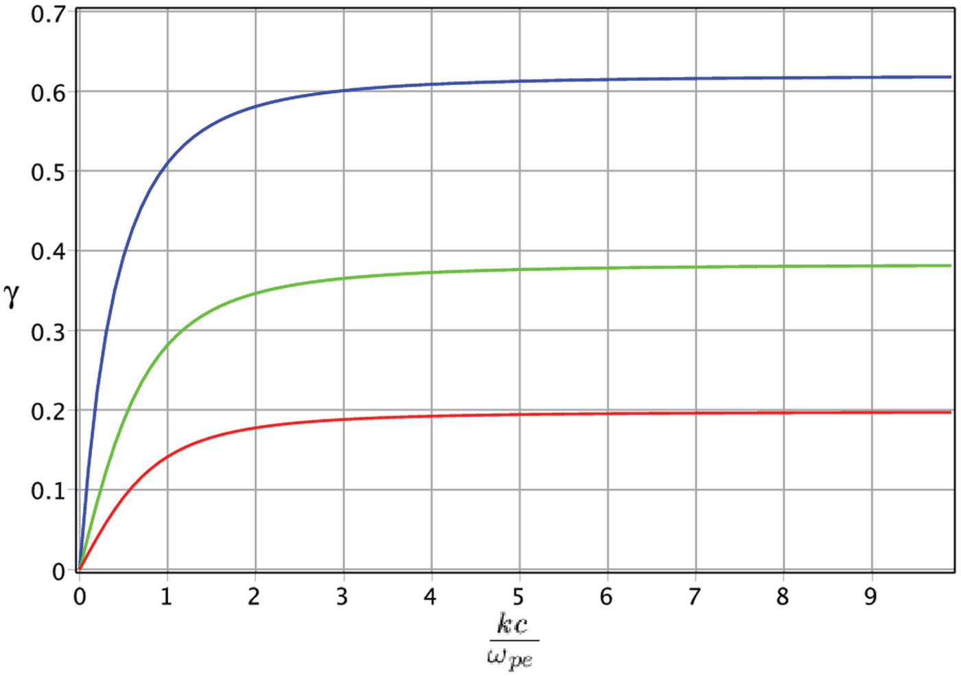
Figure 1 plots the normalized growth rate  $\gamma \, = \,\Im {\rm \omega} /{{\rm \omega} _{\rm \,pe}}$ of the filamentation instability as a function of the normalized wavenumber kc/ωpe (or the ratio of the penetration depth c/ωpe to the wavelength λ = 2π/k) computed numerically from Eq. (12), for cold and unmagnetized counterstreaming e–H − plasma. This figure shows that the instability growth rate is increased by increasing the particles drift velocity. Moreover, in the large wavenumbers limit
  ${k^2}{c^2}\;{\rm \gg}\; {\rm \omega} _{{\rm pe}}^2 $, and for weakly relativistic case (small β) the instability growth rate saturates to γ → β. Note that Figure 1 does not change with or without the ions contribution, significantly. It may be important to note that the analytical results obtained from Eq. (14) are in excellent agreement with the numerical computation of Eq. (12) plotted in Figure 1.

Fig. 1. Filamentation instability growth rate as a function of kc/ωpe for cold and unmagnetized counterstreaming e–H− plasma when the influence of H− ions is ignored (η = 0). The red, green, and blue lines are for β = 0.2, 0.4, and 0.8, respectively.
Physically speaking, when the electron current filaments are created, the magnetic fields grow linearly due to mutual attraction of these filaments. When the current filaments sufficiently close to gather, the force of the pressure gradient becomes important in Eq. (5). Since the terms including δe in Eq. (12) are the result of the pressure gradient effect, the influence of the particles thermal velocity on the instability growth rate is depicted in Figure 2 for δe = 0.2. It is seen from this figure that not only the maximum growth rate is decreased, but also the instability happens just for a finite interval of wavenumbers. The numerical solution indicates that the cut-off frequency and the maximum growth rate are decreased with increasing δe.
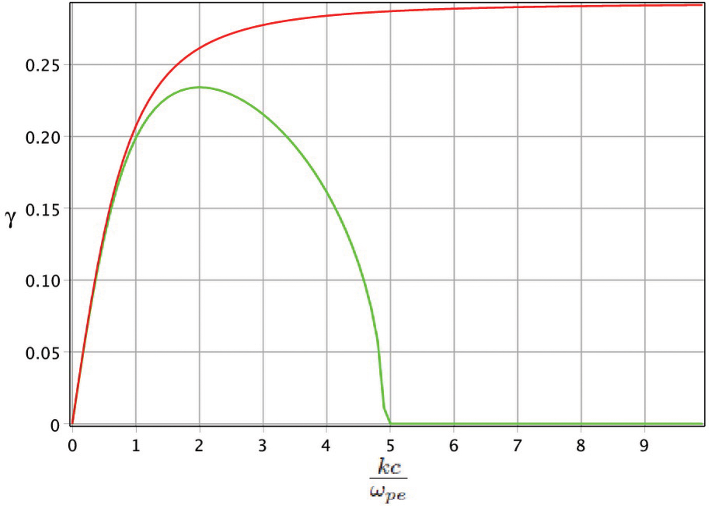
Fig. 2. Filamentation instability growth rate as a function of kc/ωpe for unmagnetized counterstreaming e–H− plasma in the absence of H− ions contribution for β = 0.3, computed numerically from Eq. (12). The green and red lines are for δe = 0.2 and δe = 0, respectively.
Figure 3 demonstrates the influence of the H− ions current filaments contribution on the instability growth rate for counterstreaming unmagnetized e–H− plasma. As shown in Figure 3 (point line) the cut-off frequency is extended upon to the large values, when the H− ion contribution is included. This means that the penetration depth of the sheared magnetic field into the plasma is increased, when the heavy H− ions begin to get involved in the instability process. As a result, the H− ions form current filaments that are responsible to the deep penetrating of sheared magnetic into the plasma.

Fig. 3. Filamentation instability growth rate as a function of kc/ωpe for unmagnetized counterstreaming e–H− plasma in the absence [solid line (η = 0)] and presence of H− ions contribution [point line (η = 1/1838)], based on the numerical solution of Eq. (12).
Figure 4 compares the instability growth rate  ${\rm \gamma} \, = \,\Im {\rm \omega} /{{\rm \omega}_{\rm \,pe}\comma}$ for magnetized and unmagnetized counterstreaming e–H− plasma in terms of kc/ωpe. The results show that by applying a magnetic field: (a) The instability growth rate and cut-off frequency are sufficiently decreased, (b) the required threshold wavenumber for the development of the filamentation instability is increased with the increasing magnetic field strength. Hence, the external magnetic field decreases the instability growth rate and constrains further the finite interval of wavenumbers. The results of the analytical and numerical solutions are in good conformity. For example, for parameters β = 0.3, η = 0, δe = 0, z = 2, maximum magnetic field strength for instability development is found around ωce ≈ 0.25ωpe from both Eqs. (12) and (16).

Fig. 4. Filamentation instability growth rate as a function of kc/ωpe for a magnetized counterstreaming e–H− plasma for β = 0.3, δe = 0.2, based on the numerical solution of Eq. (12). The red, green, and blue line are for ωce/ωpe = 0, 0.2, and 0.23, respectively.
In Figure 5 we are going to explain the influence of H− ions filaments with more detail, in magnetized counterstreaming e–H− plasma. This figure plots the instability growth rate  ${\rm \gamma} \, = \,\Im {\rm \omega} /{{\rm \omega}_{\rm \,pe}}$ as a function of kc/ωpe. The red and green lines are plotted for ωce/ωpe = 0.23 in the absence and presence of the H− ion contribution, respectively. Obviously, the threshold and cut-off frequencies extension are completely perceptible, when the H− ions filaments come into play. The numerical solution reveals that when the strength of the external magnetic field is increased upon to ωce/ωpe = 0.3, the contribution of electrons on the instability development completely lacks. Consequently, the blue line in Figure 5 shows just the H− ion contribution on the instability process. As shown in Figure 5, although the maximum growth rate is very small, the instability covers a wide range of wavenumbers. Therefore, we expect that the filamentation instability is further amplified and as a result the sheared magnetic field deeply penetrates into the plasma owing to H− ion streams, on a time scale much longer than the plasma period
  $t\;{\rm \gg}\; {\rm \omega} _{{\rm pe}}^{ - 1} $.

Fig. 5. Filamentation instability growth rate for a magnetized counterstreaming e–H− plasma as a function of kc/ωpe for β = 0.3, δe = 0.2, and ωce/ωpe = 0.23. The red and green lines are plotted in the absence (η = 0) and presence (η = 1/1838) of H− ions contribution, respectively. The blue line is for counterstreaming e–H− plasma and ωce/ωpe = 0.3.
The instability growth rate  ${\rm \gamma} \, = \,\Im {\rm \omega} /{{\rm \omega} _{\rm \,pe}}$ in terms of ωce/ωpe is shown in Figure 6, in the presence and absence of the H− ions contribution. The figure approves our claim that the instability is suppressed by applying a weak magnetic field ωce/ωpe ≈ 0.3, when the H− ion contribution is missed. On the other hand, the instability exists with a small growth rate in the presence of a very strong external magnetic field, when the H− ion filaments get involved. Subsequently, after a long time scale (
 $t\;{\rm \gg}\; {\rm \omega} _{{\rm pe}}^{ - 1} $) it is possible for the sheared magnetic field to become strong enough to deflect the electrons filaments again and amplifies the instability.

Fig. 6. Filamentation instability growth rate for a magnetized counterstreaming e–H− plasma as a function of ωce/ωpe for β = 0.3, δe = 0.2, kc/ωpe = 2. The point and solid lines are plotted in the absence (η = 0) and presence (η = 1/1838) of H− ions contribution, respectively.
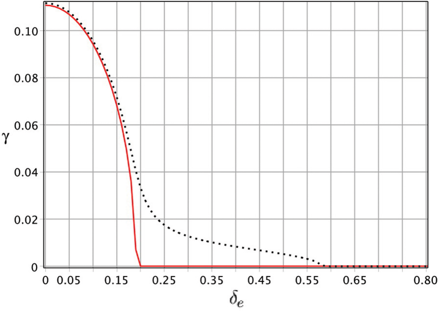
Figure 7 indicates the variation of the instability growth rate  ${\rm \gamma} \, = \,\Im {\rm \omega} /{{\rm \omega} _{\rm \,pe}}$ against δe = v the/v 0. Here, we suppose that the temperature of electrons and H− ions are equal (v thi/v the = η). As this figure demonstrates for a given external magnetic field, increasing the particles thermal velocity up to the value larger than a critical value can suppress instability generation. We find from this figure that increasing external magnetic field strength reduces this critical value, while it will be increased when the H− ion contribution gets involved in the instability process (pointed lines).

Fig. 7. Filamentation instability growth rate for a magnetized counterstreaming e–H− plasma as a function of δe for β = 0.3, kc/ωpe = 2, ωce/ωpe = 0.25. The red and point lines are plotted in the absence (η = 0) and presence (η = 1/1838) of H− ion contribution, respectively.
4. SUMMARY AND CONCLUSION
We have discussed the CF instability driven by counterstreaming e–H− plasma propagating parallel to an ambient external magnetic field. We have focused our attention on the influences of the heavy H− ions contribution, the particles thermal velocity, and the external magnetic field on the instability process. The dispersion relation is derived by using a relativistic two-fluid model and Maxwell equations. We present a analytical solution for two limiting cases (a) cold and unmagnetized counterstreaming e–H− plasma (b) cold and magnetized counterstreaming e–H− plasma propagating parallel to an ambient external magnetic field, when the influence of heavy H− ions is ignored. In order to obtain a complete solution we solved the dispersion relation numerically. Both numerical and analytical solutions admitted generation of purely growing electromagnetic perturbation across the ambient magnetic field. In addition, both solutions, with same accuracy, approved that for unmagnetized counterstreaming e–H− plasma with non-thermal particles T α → 0, the instability growth rate saturates to γ → β which is in good agreement with previous analytical investigations (Shokri & Ghorbanalilu, Reference Shokri and Ghorbanalilu2004a; Reference Shokri and Ghorbanalilu2004b). The stability analysis revealed that when the particles have nonzero thermal velocity δα ≠ 0 (or T α ≠ 0), the maximum growth rate is decreased and an instability develops in a finite interval of wavenumbers. It was shown that when the heavy H− ions got involved in the instability process, the cut-off frequency was extended. The numerical investigation showed that for a magnetized electron plasma flow: (a) The maximum growth rate and cut-off frequency were decreased, (b) the required threshold wavenumber of filamentation instability development was increased, with increasing magnetic field strength. Consequently, the instability is more constrained by applying an external magnetic field in a finite interval of wavenumbers. The influence of ion filaments was very dominant for magnetized counterstreaming e–H− plasma. It was shown that for a magnetized counterstreaming e–H− plasma, in the absence of role of H− ion, the CF instability was suppressed by applying a weak external magnetic field ( ${\rm \omega} _{{\rm ce}}^2 {\rm \ll} {\rm \omega} _{{\rm pe}}^2 $). However, the instability occurred with a small growth rate even in the presence of very strong external magnetic fields (
 ${\rm \omega} _{{\rm ce}}^2 \;{\rm \gg}\; {\rm \omega} _{{\rm pe}}^2 $), when the influence of heavy H− ions is included. As a result and an important remark, although the growth rate of instability is small for strongly magnetized counterstreaming e–H− plasma, the instability covers a wide range of wavenumbers. This means that the filamentation instability is further amplified and the sheared magnetic field deeply penetrates into the plasma owing to H− ion streams, on a time scale much longer than the plasma period
  $t\;{\rm \gg}\; {\rm \omega} _{{\rm pe}}^{ - 1} $ (Ardaneh et al., Reference Ardaneh, Cai and Nishikawa2014).