1 Introduction
The prospects for creating electron–positron pair plasmas magnetically confined in dipole or stellarator geometries have been discussed since the early 2000s (Pedersen et al.
Reference Pedersen, Boozer, Dorland, Kremer and Schmitt2003, Reference Pedersen, Danielson, Hugenschmidt, Marx, Sarasola, Schauer, Schweikhard, Surko and Winkler2012). In the near future, the first experiment aiming at this goal will be constructed (Saitoh et al.
Reference Saitoh, Stanja, Stenson, Hergenhahn, Niemann, Pedersen, Stoneking, Piochacz and Hugenschmidt2015). It is planned to confine electron–positron plasmas in a cylindrical an approximately 20 litre vacuum vessel with a levitated coil. The electrons are to be injected with an electron gun and the positrons will be supplied from the research neutron source at the Technical University of Munich. One expects the following plasma parameters: plasma density in the range
 $10^{10}~\text{m}^{-3}<n<10^{12}~\text{m}^{-3}$
, temperature in the range
$10^{10}~\text{m}^{-3}<n<10^{12}~\text{m}^{-3}$
, temperature in the range
 $1~\text{eV}<T<10~\text{eV}$
, Debye length
$1~\text{eV}<T<10~\text{eV}$
, Debye length
 $\unicode[STIX]{x1D706}_{D}=\sqrt{\unicode[STIX]{x1D716}_{0}T/(2ne^{2})}<10^{-2}~\text{m}$
and gyroradius
$\unicode[STIX]{x1D706}_{D}=\sqrt{\unicode[STIX]{x1D716}_{0}T/(2ne^{2})}<10^{-2}~\text{m}$
and gyroradius
 $\unicode[STIX]{x1D70C}\ll \unicode[STIX]{x1D706}_{D}$
. Recently, efficient injection and trapping of a cold positron beam in a dipole magnetic field configuration has been demonstrated by Saitoh et al. (Reference Saitoh, Stanja, Stenson, Hergenhahn, Niemann, Pedersen, Stoneking, Piochacz and Hugenschmidt2015). This result is a key step towards the ultimate aim of creating and studying of the first man-made magnetically confined pair plasma in the laboratory.
$\unicode[STIX]{x1D70C}\ll \unicode[STIX]{x1D706}_{D}$
. Recently, efficient injection and trapping of a cold positron beam in a dipole magnetic field configuration has been demonstrated by Saitoh et al. (Reference Saitoh, Stanja, Stenson, Hergenhahn, Niemann, Pedersen, Stoneking, Piochacz and Hugenschmidt2015). This result is a key step towards the ultimate aim of creating and studying of the first man-made magnetically confined pair plasma in the laboratory.
It has been shown by Helander (Reference Helander2014) that pair plasmas possess unique gyrokinetic stability properties thanks to the mass symmetry between the particle species. For example, drift instabilities are completely absent in straight unsheared geometry, e.g. in a slab. They can be destabilised only in the presence of magnetic curvature in more complicated confining fields. Helander & Connor (Reference Helander and Connor2016) found that this result persists also in the electromagnetic regime. However, what happens if the perfect mass symmetry between the positively charged particles (positrons) and the negatively charged ones (electrons) is broken? This can happen if some fraction of ions (e.g. protons) is introduced into the pair plasma, which will probably be the case in experiments since the pumping and vacuum systems are never completely perfect. Then one could expect that the drift instabilities will reappear.
In this paper, we address the effect of proton contamination on the gyrokinetic stability of pair plasmas. We find that drift instabilities can indeed appear in contaminated pair plasmas if the proton fraction exceeds some threshold. Also, we find that the shear Alfvén wave is present in a contaminated plasma even if the ion contamination is small. Its frequency, however, increases rapidly when the ion fraction becomes negligible.
Table 1. Gyrokinetic modes in slab geometry. The mode name appears in the first column. The second column indicates whether the mode is stable or not. For unstable modes, the destabilising gradient is written. The third column indicates if the mode requires an electromagnetic component to exist or if the electrostatic perturbation is sufficient. In pure pair plasmas, only K-modes of the electron type exist. Other modes require some degree of proton contamination.

The structure of the paper is as follows. In § 2, the general electromagnetic dispersion relation is derived. It describes slab gyrokinetic stability in plasmas with an arbitrary number of species, although we consider only three species in this work. Solutions of this dispersion relation can be classified with respect to the driving gradient, stability and nature of the perturbations (electrostatic or electromagnetic). A brief summary of the modes existing in a shearless slab is given in table 1. In § 3, the stable part of the gyrokinetic spectrum (K-modes) is addressed. In §§ 4, 5 and 6, drift instabilities in three-component plasmas are considered. In § 7, the shear Alfvén wave in electron–positron–ion plasmas is described. Conclusions are summarised in § 8.
2 Dispersion relation
Following Helander (Reference Helander2014) and Helander & Connor (Reference Helander and Connor2016), we use gyrokinetic theory to analyse the linear stability of electron–positron–ion plasmas. It is convenient to write the gyrokinetic distribution function in the form:
 $$\begin{eqnarray}f_{a}=f_{a0}\left(1-\frac{e_{a}\unicode[STIX]{x1D719}}{T_{a}}\right)+g_{a}=f_{a0}+f_{a1},\quad f_{a1}=-\frac{e_{a}\unicode[STIX]{x1D719}}{T_{a}}\,f_{a0}+g_{a}.\end{eqnarray}$$
Here,
 $f_{a0}$
is a Maxwellian,
$f_{a0}$
is a Maxwellian,
 $a$
is the species index with
$a$
is the species index with
 $a=e$
corresponding to electrons,
$a=e$
corresponding to electrons,
 $a=p$
to positrons and
$a=p$
to positrons and
 $a=i$
to the ions,
$a=i$
to the ions,
 $e_{a}$
is the electric charge,
$e_{a}$
is the electric charge,
 $f_{a1}$
is the perturbed part of the distribution function and
$f_{a1}$
is the perturbed part of the distribution function and
 $g_{a}$
is the non-adiabatic part of
$g_{a}$
is the non-adiabatic part of
 $f_{a1}$
. The linearised gyrokinetic equation in this notation is
$f_{a1}$
. The linearised gyrokinetic equation in this notation is
 $$\begin{eqnarray}\text{i}v_{\Vert }\unicode[STIX]{x1D735}_{\Vert }g_{a}+(\unicode[STIX]{x1D714}-\unicode[STIX]{x1D714}_{\text{d}a})g_{a}=\frac{e_{a}}{T_{a}}\,\text{J}_{0}\left(\frac{k_{\bot }v_{\bot }}{\unicode[STIX]{x1D714}_{\text{c}a}}\right)\,(\unicode[STIX]{x1D714}-\unicode[STIX]{x1D714}_{\ast a}^{T})\,(\unicode[STIX]{x1D719}-v_{\Vert }A_{\Vert })\,f_{a0}\end{eqnarray}$$
with
 $\text{J}_{0}$
the Bessel function,
$\text{J}_{0}$
the Bessel function,
 $\unicode[STIX]{x1D714}$
the complex frequency of the mode,
$\unicode[STIX]{x1D714}$
the complex frequency of the mode,
 $\unicode[STIX]{x1D714}_{\text{c}a}$
the cyclotron frequency,
$\unicode[STIX]{x1D714}_{\text{c}a}$
the cyclotron frequency,
 $k_{\bot }$
the perpendicular wavenumber,
$k_{\bot }$
the perpendicular wavenumber,
 $v_{\Vert }$
and
$v_{\Vert }$
and
 $v_{\bot }$
the parallel and perpendicular velocities,
$v_{\bot }$
the parallel and perpendicular velocities,
 $\unicode[STIX]{x1D719}$
the perturbed electrostatic potential and
$\unicode[STIX]{x1D719}$
the perturbed electrostatic potential and
 $A_{\Vert }$
the perturbed parallel magnetic potential in the Coulomb gauge. We consider an unsheared slab geometry with the coordinates
$A_{\Vert }$
the perturbed parallel magnetic potential in the Coulomb gauge. We consider an unsheared slab geometry with the coordinates
 $(x,y,z)$
, a uniform magnetic field
$(x,y,z)$
, a uniform magnetic field
 $\boldsymbol{B}=B\boldsymbol{e}_{z}$
pointing in the
$\boldsymbol{B}=B\boldsymbol{e}_{z}$
pointing in the
 $z$
-direction and plasma profiles which are non-uniform in the
$z$
-direction and plasma profiles which are non-uniform in the
 $x$
-direction. In slab geometry, the drift frequency
$x$
-direction. In slab geometry, the drift frequency
 $\unicode[STIX]{x1D714}_{\text{d}a}=0$
. Other notations used are
$\unicode[STIX]{x1D714}_{\text{d}a}=0$
. Other notations used are
 $$\begin{eqnarray}\displaystyle & \displaystyle \unicode[STIX]{x1D714}_{\ast a}^{T}=\unicode[STIX]{x1D714}_{\ast a}\left[1+\unicode[STIX]{x1D702}_{a}\left(\frac{v^{2}}{v_{\text{th}a}^{2}}-\frac{3}{2}\right)\right],\quad v=\sqrt{v_{\Vert }^{2}+v_{\bot }^{2}},\quad k_{\bot }=\sqrt{k_{x}^{2}+k_{y}^{2}} & \displaystyle\end{eqnarray}$$
 $$\begin{eqnarray}\displaystyle & \displaystyle \unicode[STIX]{x1D714}_{\ast a}=\frac{k_{y}T_{a}}{e_{a}B}\frac{\text{d}\ln n_{a}}{\text{d}x},\quad \unicode[STIX]{x1D702}_{a}=\frac{\text{d}\ln T_{a}}{\text{d}\ln n_{a}},\quad v_{\text{th}a}=\sqrt{\frac{2T_{a}}{m_{a}}}. & \displaystyle\end{eqnarray}$$
Here,
 $m_{a}$
is the particle mass,
$m_{a}$
is the particle mass,
 $n_{a}$
is the ambient particle density and the sign convention is such that
$n_{a}$
is the ambient particle density and the sign convention is such that
 $\unicode[STIX]{x1D714}_{\ast i}\leqslant 0$
,
$\unicode[STIX]{x1D714}_{\ast i}\leqslant 0$
,
 $\unicode[STIX]{x1D714}_{\ast p}\leqslant 0$
and
$\unicode[STIX]{x1D714}_{\ast p}\leqslant 0$
and
 $\unicode[STIX]{x1D714}_{\ast e}\geqslant 0$
. For simplicity, we will assume
$\unicode[STIX]{x1D714}_{\ast e}\geqslant 0$
. For simplicity, we will assume
 $k_{x}=0$
and
$k_{x}=0$
and
 $k_{\bot }=k_{y}$
throughout the paper. Taking the Fourier transform along the parallel coordinate, we obtain:
$k_{\bot }=k_{y}$
throughout the paper. Taking the Fourier transform along the parallel coordinate, we obtain:
 $$\begin{eqnarray}(\unicode[STIX]{x1D714}-k_{\Vert }v_{\Vert })g_{a}=\frac{e_{a}}{T_{a}}\,\text{J}_{0}\left(\frac{k_{\bot }v_{\bot }}{\unicode[STIX]{x1D714}_{\text{c}a}}\right)(\unicode[STIX]{x1D714}-\unicode[STIX]{x1D714}_{\ast a}^{T})(\unicode[STIX]{x1D719}-v_{\Vert }A_{\Vert })\,f_{a0}.\end{eqnarray}$$
This equation is trivially solved:
 $$\begin{eqnarray}g_{a}=\frac{\unicode[STIX]{x1D714}-\unicode[STIX]{x1D714}_{\ast a}^{T}}{\unicode[STIX]{x1D714}-k_{\Vert }v_{\Vert }}\frac{e_{a}f_{a0}}{T_{a}}\text{J}_{0}(\unicode[STIX]{x1D719}-v_{\Vert }A_{\Vert }).\end{eqnarray}$$
The gyrokinetic quasineutrality condition and the parallel Ampere’s law are
 $$\begin{eqnarray}\left(\mathop{\sum }_{a}\frac{n_{a}e_{a}^{2}}{T_{a}}+\unicode[STIX]{x1D716}_{0}\,k_{\bot }^{2}\right)\unicode[STIX]{x1D719}=\mathop{\sum }_{a}e_{a}\int g_{a}\text{J}_{0}\,\text{d}^{3}v,\quad A_{\Vert }=\frac{\unicode[STIX]{x1D707}_{0}}{k_{\bot }^{2}}\mathop{\sum }_{a}e_{a}\int v_{\Vert }g_{a}\text{J}_{0}\,\text{d}^{3}v.\end{eqnarray}$$
Here,
 $\unicode[STIX]{x1D716}_{0}$
is the electric permittivity and
$\unicode[STIX]{x1D716}_{0}$
is the electric permittivity and
 $\unicode[STIX]{x1D707}_{0}$
is the magnetic permeability of free space. For the electromagnetic dispersion relation, it is convenient to define:
$\unicode[STIX]{x1D707}_{0}$
is the magnetic permeability of free space. For the electromagnetic dispersion relation, it is convenient to define:
 $$\begin{eqnarray}W_{na}=-\frac{1}{n_{a}v_{\text{th}a}^{n}}\int \frac{\unicode[STIX]{x1D714}-\unicode[STIX]{x1D714}_{\ast a}^{T}}{\unicode[STIX]{x1D714}-k_{\Vert }v_{\Vert }}\text{J}_{0}^{2}\,f_{a0}\,v_{\Vert }^{n}\,\text{d}^{3}v.\end{eqnarray}$$
Taking velocity-space integrals, one finds:
 $$\begin{eqnarray}W_{na}=\unicode[STIX]{x1D701}_{a}\left\{\left(1-\frac{\unicode[STIX]{x1D714}_{\ast a}}{\unicode[STIX]{x1D714}}\right)Z_{na}\unicode[STIX]{x1D6E4}_{0a}+\frac{\unicode[STIX]{x1D714}_{\ast a}\unicode[STIX]{x1D702}_{a}}{\unicode[STIX]{x1D714}}\,\left[\frac{3}{2}Z_{na}\unicode[STIX]{x1D6E4}_{0a}-Z_{na}\unicode[STIX]{x1D6E4}_{\ast a}-Z_{n+2,a}\unicode[STIX]{x1D6E4}_{0a}\right]\right\}.\end{eqnarray}$$
Here, the following notation is employed:
 $$\begin{eqnarray}\displaystyle & \displaystyle \frac{1}{\unicode[STIX]{x1D706}_{\text{D}a}^{2}}=\frac{e_{a}^{2}n_{a}}{\unicode[STIX]{x1D716}_{0}T_{a}},\quad \frac{1}{\unicode[STIX]{x1D706}_{\text{D}}^{2}}=\mathop{\sum }_{a}\frac{1}{\unicode[STIX]{x1D706}_{\text{D}a}^{2}},\quad b_{a}=k_{\bot }^{2}\unicode[STIX]{x1D70C}_{a}^{2},\quad \unicode[STIX]{x1D70C}_{a}=\frac{\sqrt{m_{a}T_{a}}}{|e_{a}|B} & \displaystyle\end{eqnarray}$$
 $$\begin{eqnarray}\displaystyle & \displaystyle \unicode[STIX]{x1D6E4}_{\ast a}=\unicode[STIX]{x1D6E4}_{0a}-b_{a}[\unicode[STIX]{x1D6E4}_{0a}-\unicode[STIX]{x1D6E4}_{1a}],\quad \unicode[STIX]{x1D6E4}_{0a}=\text{I}_{0}(b_{a})\text{e}^{-b_{a}},\,\unicode[STIX]{x1D6E4}_{1a}=I_{1}(b_{a})\text{e}^{-b_{a}} & \displaystyle\end{eqnarray}$$
 $$\begin{eqnarray}\displaystyle & \displaystyle Z_{na}=\frac{1}{\sqrt{\unicode[STIX]{x03C0}}}\int _{-\infty }^{\infty }\frac{x^{n}\text{e}^{-x^{2}}\text{d}x}{x-\unicode[STIX]{x1D701}_{a}},\quad \unicode[STIX]{x1D701}_{a}=\frac{\unicode[STIX]{x1D714}}{k_{\Vert }v_{\text{th}a}} & \displaystyle\end{eqnarray}$$
with
 $\text{I}_{0}$
and
$\text{I}_{0}$
and
 $\text{I}_{1}$
denoting the modified Bessel functions of the first kind. Using this notation, we can cast the field equations into the form:
$\text{I}_{1}$
denoting the modified Bessel functions of the first kind. Using this notation, we can cast the field equations into the form:
 $$\begin{eqnarray}\displaystyle & \displaystyle (1+k_{\bot }^{2}\unicode[STIX]{x1D706}_{D}^{2})\unicode[STIX]{x1D719}+\mathop{\sum }_{a}\frac{\unicode[STIX]{x1D706}_{D}^{2}}{\unicode[STIX]{x1D706}_{Da}^{2}}(W_{0a}\,\unicode[STIX]{x1D719}-W_{1a}\,A_{\Vert }v_{\text{th}a})=0 & \displaystyle\end{eqnarray}$$
 $$\begin{eqnarray}\displaystyle & \displaystyle A_{\Vert }+\frac{1}{c^{2}}\mathop{\sum }_{a}\frac{v_{\text{th}a}}{k_{\bot }^{2}\unicode[STIX]{x1D706}_{Da}^{2}}(W_{1a}\,\unicode[STIX]{x1D719}-W_{2a}\,A_{\Vert }v_{\text{th}a})=0. & \displaystyle\end{eqnarray}$$
Computing the determinant of this system of equations, we find the electromagnetic dispersion relation describing an electron–positron–ion plasma in a slab geometry:
 $$\begin{eqnarray}\displaystyle & & \displaystyle \displaystyle \left(1+k_{\bot }^{2}\unicode[STIX]{x1D706}_{D}^{2}+\mathop{\sum }_{a}\frac{\unicode[STIX]{x1D706}_{D}^{2}}{\unicode[STIX]{x1D706}_{Da}^{2}}\,W_{0a}\right)\left(1-2\mathop{\sum }_{a}\frac{\unicode[STIX]{x1D6FD}_{a}}{k_{\bot }^{2}\unicode[STIX]{x1D70C}_{a}^{2}}\,W_{2a}\right)\nonumber\\ \displaystyle & & \displaystyle \displaystyle \quad +\,2\mathop{\sum }_{a}\frac{\unicode[STIX]{x1D706}_{D}^{2}}{\unicode[STIX]{x1D706}_{Da}^{2}}\;W_{1a}v_{\text{th}a}\mathop{\sum }_{a}\frac{\unicode[STIX]{x1D6FD}_{a}}{k_{\bot }^{2}\unicode[STIX]{x1D70C}_{a}^{2}}\;\frac{W_{1a}}{v_{\text{th}a}}=0.\end{eqnarray}$$
Here,
 $\unicode[STIX]{x1D6FD}_{a}=\unicode[STIX]{x1D707}_{0}n_{a}T_{a}/B^{2}$
. The electrostatic limit corresponds, as usual, to
$\unicode[STIX]{x1D6FD}_{a}=\unicode[STIX]{x1D707}_{0}n_{a}T_{a}/B^{2}$
. The electrostatic limit corresponds, as usual, to
 $\unicode[STIX]{x1D6FD}_{a}=0$
.
$\unicode[STIX]{x1D6FD}_{a}=0$
.
In the following, we will use this dispersion relation in order to describe instabilities which can appear in three-component plasmas. This will give us insight into the general properties of the gyrokinetic stability of such plasmas.
3 Gyrokinetic stable modes
We first consider the case of a pure electrostatic electron–positron plasma. Assuming quasineutrality
 $\unicode[STIX]{x1D714}_{\ast p}=-\unicode[STIX]{x1D714}_{\ast e}$
, equal temperatures
$\unicode[STIX]{x1D714}_{\ast p}=-\unicode[STIX]{x1D714}_{\ast e}$
, equal temperatures
 $T_{p}=T_{e}$
and equal temperature gradients
$T_{p}=T_{e}$
and equal temperature gradients
 $\unicode[STIX]{x1D702}_{p}=\unicode[STIX]{x1D702}_{e}$
, we can reduce the dispersion relation to
$\unicode[STIX]{x1D702}_{p}=\unicode[STIX]{x1D702}_{e}$
, we can reduce the dispersion relation to
 $$\begin{eqnarray}1+k_{\bot }^{2}\unicode[STIX]{x1D706}_{\text{D}}^{2}+\unicode[STIX]{x1D701}Z_{0}=0\end{eqnarray}$$
with the electron and positron finite Larmor radius (FLR) effects neglected for simplicity, implying that
 $\unicode[STIX]{x1D6E4}_{0e}=\unicode[STIX]{x1D6E4}_{0p}=1$
. Here, we use the notation
$\unicode[STIX]{x1D6E4}_{0e}=\unicode[STIX]{x1D6E4}_{0p}=1$
. Here, we use the notation
 $Z_{0}=Z_{0e}=Z_{0p}$
and
$Z_{0}=Z_{0e}=Z_{0p}$
and
 $\unicode[STIX]{x1D701}=\unicode[STIX]{x1D701}_{e}=\unicode[STIX]{x1D701}_{p}$
. Equations of this type have been considered in detail by Fried & Gould (Reference Fried and Gould1961) and Yegorenkov & Stepanov (Reference Yegorenkov and Stepanov1987, Reference Yegorenkov and Stepanov1988) for conventional (hydrogen) plasmas. In a hydrogen plasma, equation (3.2), similar to (3.1), describes the plasma stability in the absence of the density and temperature gradients for
$\unicode[STIX]{x1D701}=\unicode[STIX]{x1D701}_{e}=\unicode[STIX]{x1D701}_{p}$
. Equations of this type have been considered in detail by Fried & Gould (Reference Fried and Gould1961) and Yegorenkov & Stepanov (Reference Yegorenkov and Stepanov1987, Reference Yegorenkov and Stepanov1988) for conventional (hydrogen) plasmas. In a hydrogen plasma, equation (3.2), similar to (3.1), describes the plasma stability in the absence of the density and temperature gradients for
 $T_{i}=T_{e}$
:
$T_{i}=T_{e}$
:
 $$\begin{eqnarray}1+k_{\bot }^{2}\unicode[STIX]{x1D706}_{\text{D}}^{2}+{\textstyle \frac{1}{2}}\left[\unicode[STIX]{x1D701}_{i}Z_{0}(\unicode[STIX]{x1D701}_{i})\unicode[STIX]{x1D6E4}_{0i}+\unicode[STIX]{x1D701}_{e}Z_{0}(\unicode[STIX]{x1D701}_{e})\unicode[STIX]{x1D6E4}_{0e}\right]=0.\end{eqnarray}$$
This equation has an infinite number of solutions, called K-modes (Yegorenkov & Stepanov Reference Yegorenkov and Stepanov1987, Reference Yegorenkov and Stepanov1988). These modes can be of the ion type with
 $\unicode[STIX]{x1D701}_{i}\geqslant 1$
and
$\unicode[STIX]{x1D701}_{i}\geqslant 1$
and
 $\unicode[STIX]{x1D701}_{e}\ll 1$
, or of the electron type with
$\unicode[STIX]{x1D701}_{e}\ll 1$
, or of the electron type with
 $\unicode[STIX]{x1D701}_{e}\geqslant 1$
. In figure 1, the spectrum resulting from (3.2) for the conventional plasma is plotted including K-modes of the ion type. This spectrum was computed numerically using the Nyquist technique (Carpentier & Santos Reference Carpentier and Santos1982; Davies Reference Davies1986). The staircase-like visual appearance of figures 1 and 2 is an artefact caused by the density of the roots of the dispersion relation increasing towards the origin of the coordinates. This complicates the numerical solution in this area.
$\unicode[STIX]{x1D701}_{e}\geqslant 1$
. In figure 1, the spectrum resulting from (3.2) for the conventional plasma is plotted including K-modes of the ion type. This spectrum was computed numerically using the Nyquist technique (Carpentier & Santos Reference Carpentier and Santos1982; Davies Reference Davies1986). The staircase-like visual appearance of figures 1 and 2 is an artefact caused by the density of the roots of the dispersion relation increasing towards the origin of the coordinates. This complicates the numerical solution in this area.

Figure 1. (a) Gyrokinetic frequency spectrum for conventional plasmas including sound wave and the electrostatic limit of the Alfvén wave. (b) Low-frequency part of the spectrum (K-modes of the ion type).

Figure 2. (a) The imaginary part of the spectrum in a homogeneous plasma. (b) The same in the presence of an ion temperature gradient
 $\unicode[STIX]{x1D705}_{\text{T}i}\unicode[STIX]{x1D70C}_{i}=0.1$
with
$\unicode[STIX]{x1D705}_{\text{T}i}\unicode[STIX]{x1D70C}_{i}=0.1$
with
 $\unicode[STIX]{x1D705}_{Ti}=-\text{d}\ln T_{i}/\text{d}x$
. In this figure, i-modes denote modes rotating in the ion diamagnetic direction (corresponding to the negative frequencies, recall the sign convention
$\unicode[STIX]{x1D705}_{Ti}=-\text{d}\ln T_{i}/\text{d}x$
. In this figure, i-modes denote modes rotating in the ion diamagnetic direction (corresponding to the negative frequencies, recall the sign convention
 $\unicode[STIX]{x1D714}_{\ast i}<0$
and
$\unicode[STIX]{x1D714}_{\ast i}<0$
and
 $\unicode[STIX]{x1D714}_{\ast e}>0$
) and e-modes correspond to modes rotating in the electron diamagnetic direction (positive frequencies).
$\unicode[STIX]{x1D714}_{\ast e}>0$
) and e-modes correspond to modes rotating in the electron diamagnetic direction (positive frequencies).
In figure 2, one sees that, as Fried & Gould (Reference Fried and Gould1961) suggested, most of the solutions of (3.2) are strongly damped, satisfying
 $|\unicode[STIX]{x1D6FE}|\sim |\unicode[STIX]{x1D714}|$
. The least damped solutions can be destabilised by plasma profile gradients leading either to the ion-temperature-gradient-driven instability (ITG), the electron-temperature-gradient-driven instability (ETG) or the universal instability, driven by the density gradient. This is shown in figure 2, where the effect of the ion temperature gradient on the gyrokinetic spectrum in a conventional plasma can be seen. In pure pair plasmas, however, the electron and the positron diamagnetic contributions cancel also in presence of profile gradients, making such plasmas absolutely stable in a slab geometry within the gyrokinetic description. Note however, that perfect symmetry between the electron and positron density and temperature profiles is required to guarantee the cancellation of the diamagnetic terms. While density profiles are always identical for the two species in a quasineutral plasma, the temperature profiles can differ. In this case, a pure pair plasma can be temperature-gradient unstable, as we will see in the following. The gradient-driven instabilities can also appear if a pair plasma is ‘contaminated’ by protons or other ions.
$|\unicode[STIX]{x1D6FE}|\sim |\unicode[STIX]{x1D714}|$
. The least damped solutions can be destabilised by plasma profile gradients leading either to the ion-temperature-gradient-driven instability (ITG), the electron-temperature-gradient-driven instability (ETG) or the universal instability, driven by the density gradient. This is shown in figure 2, where the effect of the ion temperature gradient on the gyrokinetic spectrum in a conventional plasma can be seen. In pure pair plasmas, however, the electron and the positron diamagnetic contributions cancel also in presence of profile gradients, making such plasmas absolutely stable in a slab geometry within the gyrokinetic description. Note however, that perfect symmetry between the electron and positron density and temperature profiles is required to guarantee the cancellation of the diamagnetic terms. While density profiles are always identical for the two species in a quasineutral plasma, the temperature profiles can differ. In this case, a pure pair plasma can be temperature-gradient unstable, as we will see in the following. The gradient-driven instabilities can also appear if a pair plasma is ‘contaminated’ by protons or other ions.
Some analytic progress can be made for K-modes in an electron–positron plasma. Assuming
 $\unicode[STIX]{x1D701}_{e}=\unicode[STIX]{x1D701}_{p}\gg 1$
and
$\unicode[STIX]{x1D701}_{e}=\unicode[STIX]{x1D701}_{p}\gg 1$
and
 $|\unicode[STIX]{x1D6FE}|\sim |\unicode[STIX]{x1D714}|$
, the plasma dispersion function can be approximated:
$|\unicode[STIX]{x1D6FE}|\sim |\unicode[STIX]{x1D714}|$
, the plasma dispersion function can be approximated:
 $$\begin{eqnarray}Z_{0}(\unicode[STIX]{x1D701}_{e})\approx 2\text{i}\sqrt{\unicode[STIX]{x03C0}}\text{e}^{-\unicode[STIX]{x1D701}_{e}^{2}}-\frac{1}{\unicode[STIX]{x1D701}_{e}}-\frac{1}{2\unicode[STIX]{x1D701}_{e}^{3}}.\end{eqnarray}$$
Using this expansion and neglecting the Debye length,
 $k_{\bot }\unicode[STIX]{x1D706}_{D}\ll 1$
, we obtain:
$k_{\bot }\unicode[STIX]{x1D706}_{D}\ll 1$
, we obtain:
 $$\begin{eqnarray}4\text{i}\sqrt{\unicode[STIX]{x03C0}}\unicode[STIX]{x1D701}_{e}^{3}\text{e}^{-\unicode[STIX]{x1D701}_{e}^{2}}=1.\end{eqnarray}$$
Introducing the notation
 $\unicode[STIX]{x1D701}_{e}=x-\text{i}y$
and assuming
$\unicode[STIX]{x1D701}_{e}=x-\text{i}y$
and assuming
 $x=\pm (y+\unicode[STIX]{x1D6E5})$
with
$x=\pm (y+\unicode[STIX]{x1D6E5})$
with
 $\unicode[STIX]{x1D6E5}\ll y$
(Yegorenkov & Stepanov Reference Yegorenkov and Stepanov1987, Reference Yegorenkov and Stepanov1988), we can write the dispersion relation in the form:
$\unicode[STIX]{x1D6E5}\ll y$
(Yegorenkov & Stepanov Reference Yegorenkov and Stepanov1987, Reference Yegorenkov and Stepanov1988), we can write the dispersion relation in the form:
 $$\begin{eqnarray}8y^{3}\sqrt{2\unicode[STIX]{x03C0}}\text{e}^{-2y\unicode[STIX]{x1D6E5}}\exp (2\text{i}y^{2}-\text{i}\unicode[STIX]{x03C0}/4)=1\equiv \exp (2\unicode[STIX]{x03C0}m\text{i}).\end{eqnarray}$$
Splitting this relation into equations for the argument and for the absolute value and employing
 $\unicode[STIX]{x1D6E5}/y\ll 1$
, we obtain:
$\unicode[STIX]{x1D6E5}/y\ll 1$
, we obtain:
 $$\begin{eqnarray}2y^{2}-\unicode[STIX]{x03C0}/4=2\unicode[STIX]{x03C0}m,\quad 8y^{3}\sqrt{2\unicode[STIX]{x03C0}}\text{e}^{-2y\unicode[STIX]{x1D6E5}}=1.\end{eqnarray}$$
Thus, an infinite family of solutions is found:
 $$\begin{eqnarray}y_{m}=\sqrt{\unicode[STIX]{x03C0}m+\unicode[STIX]{x03C0}/8}\approx \sqrt{\unicode[STIX]{x03C0}m},\quad \unicode[STIX]{x1D6E5}_{m}=\frac{\ln (8y_{m}^{3}\sqrt{2\unicode[STIX]{x03C0}})}{2y_{m}},\quad x_{m}=\pm (y_{m}+\unicode[STIX]{x1D6E5}_{m}).\end{eqnarray}$$
Finally, we write our solutions in the form:
 $$\begin{eqnarray}\unicode[STIX]{x1D714}_{m}=\pm k_{\Vert }v_{\text{th}e}x_{m},\quad \unicode[STIX]{x1D6FE}_{m}=-k_{\Vert }v_{\text{th}e}y_{m}.\end{eqnarray}$$
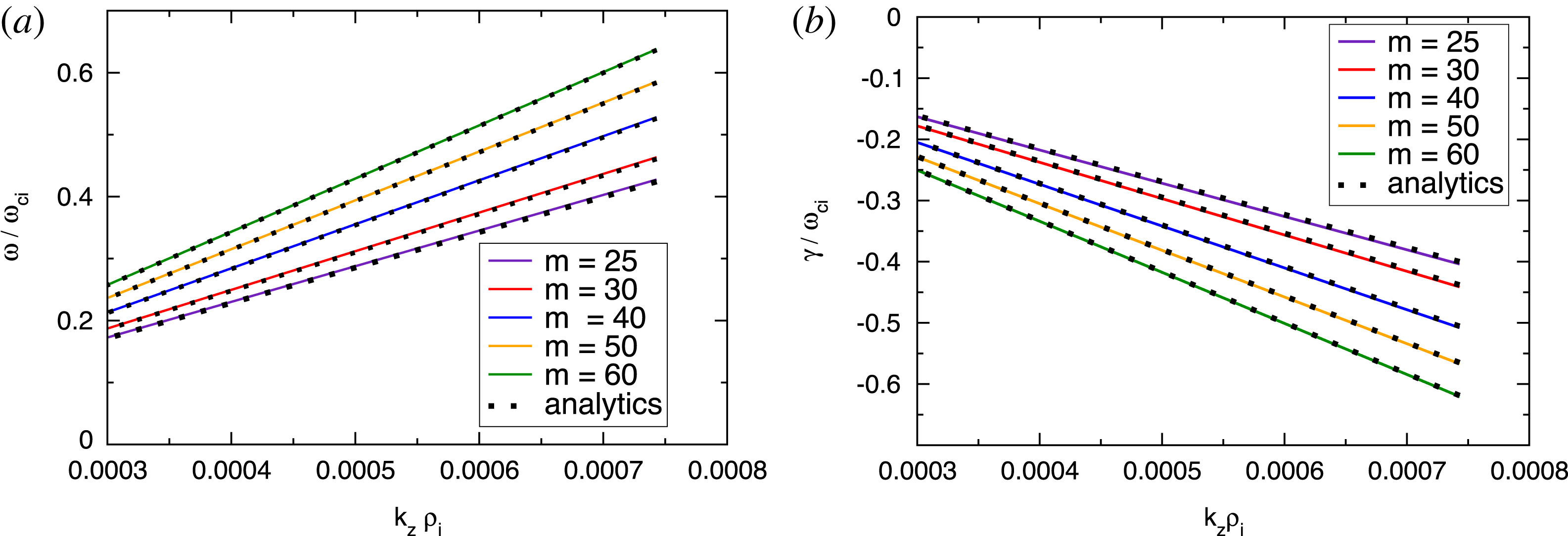
These relations describe strongly damped K-modes in a pure electron–positron plasma. In figure 3, we compare these analytic results with the numerical solution of the original dispersion relation (2.15) and find very good agreement. Note that the expansion (3.3) is valid for
 $m\gg 1$
. For low
$m\gg 1$
. For low
 $m$
, the dispersion relation must be solved numerically.
$m$
, the dispersion relation must be solved numerically.


Figure 4. ‘K-mode’ solution of the dispersion relation for conventional plasma assuming
 $k_{\bot }\unicode[STIX]{x1D706}_{D}=0$
. One can see the ion and the electron parts of the spectrum. The numerical solution of (2.15) is compared with the analytic result (3.13). For the numerical solution, we set the density and temperature gradients appearing in (2.15) to zero.
$k_{\bot }\unicode[STIX]{x1D706}_{D}=0$
. One can see the ion and the electron parts of the spectrum. The numerical solution of (2.15) is compared with the analytic result (3.13). For the numerical solution, we set the density and temperature gradients appearing in (2.15) to zero.
In a conventional hydrogen plasma, one can make the usual assumption
 $\unicode[STIX]{x1D701}_{i}\gg 1$
and
$\unicode[STIX]{x1D701}_{i}\gg 1$
and
 $\unicode[STIX]{x1D701}_{e}\ll 1$
corresponding to the K-modes of the ion type. In this case, the following expansions of the plasma dispersion function can be used:
$\unicode[STIX]{x1D701}_{e}\ll 1$
corresponding to the K-modes of the ion type. In this case, the following expansions of the plasma dispersion function can be used:
 $$\begin{eqnarray}Z_{0}(\unicode[STIX]{x1D701}_{i})=2\text{i}\sqrt{\unicode[STIX]{x03C0}}\text{e}^{-\unicode[STIX]{x1D701}_{i}^{2}}-\frac{1}{\unicode[STIX]{x1D701}_{i}}-\frac{1}{2\unicode[STIX]{x1D701}_{i}^{3}},\quad Z_{0}(\unicode[STIX]{x1D701}_{e})=\text{i}\sqrt{\unicode[STIX]{x03C0}}-2\unicode[STIX]{x1D701}_{e},\end{eqnarray}$$
which lead to the approximated dispersion relation (assuming
 $k_{\bot }\unicode[STIX]{x1D706}_{D}\ll 1$
):
$k_{\bot }\unicode[STIX]{x1D706}_{D}\ll 1$
):
 $$\begin{eqnarray}\left(1-\unicode[STIX]{x1D6E4}_{0i}/2\right)+\left(\text{i}\unicode[STIX]{x1D701}_{i}\sqrt{\unicode[STIX]{x03C0}}\text{e}^{-\unicode[STIX]{x1D701}_{i}^{2}}-\frac{1}{4\unicode[STIX]{x1D701}_{i}^{2}}\right)\unicode[STIX]{x1D6E4}_{0i}+O(\unicode[STIX]{x1D701}_{e})=0.\end{eqnarray}$$
For simplicity, we neglect FLR effects, implying
 $\unicode[STIX]{x1D6E4}_{0i}=1$
. Also, the small contribution
$\unicode[STIX]{x1D6E4}_{0i}=1$
. Also, the small contribution
 $1/(4\unicode[STIX]{x1D701}_{i}^{2})\ll 1$
can be neglected compared to the other terms. Then, we obtain:
$1/(4\unicode[STIX]{x1D701}_{i}^{2})\ll 1$
can be neglected compared to the other terms. Then, we obtain:
 $$\begin{eqnarray}2\text{i}\unicode[STIX]{x1D701}_{i}\sqrt{\unicode[STIX]{x03C0}}\text{e}^{-\unicode[STIX]{x1D701}_{i}^{2}}+1=0.\end{eqnarray}$$
Using the notation
 $\unicode[STIX]{x1D701}_{i}=x-\text{i}y$
with
$\unicode[STIX]{x1D701}_{i}=x-\text{i}y$
with
 $x=\pm (y+\unicode[STIX]{x1D6E5})$
and employing
$x=\pm (y+\unicode[STIX]{x1D6E5})$
and employing
 $\unicode[STIX]{x1D6E5}\ll 1$
, we can split the dispersion relation into equations for the argument and for the absolute value:
$\unicode[STIX]{x1D6E5}\ll 1$
, we can split the dispersion relation into equations for the argument and for the absolute value:
 $$\begin{eqnarray}2y\sqrt{2\unicode[STIX]{x03C0}}\text{e}^{-2y\unicode[STIX]{x1D6E5}}\exp (2\text{i}y^{2}-3\unicode[STIX]{x03C0}\text{i}/4)=1\equiv \exp (2\unicode[STIX]{x03C0}m\text{i}).\end{eqnarray}$$
Finally, the solutions for the K-modes of the ion type are
 $$\begin{eqnarray}y_{m}=\sqrt{\unicode[STIX]{x03C0}m+\frac{3\unicode[STIX]{x03C0}}{8}}\approx \sqrt{\unicode[STIX]{x03C0}m},\quad \unicode[STIX]{x1D6E5}_{m}=\frac{\ln (2y\sqrt{2\unicode[STIX]{x03C0}})}{2y},\quad x_{m}=\pm (y_{m}+\unicode[STIX]{x1D6E5}_{m}).\end{eqnarray}$$
In figure 4, these analytic results are compared with the numerical solution of the original (exact) dispersion relation (2.15).
Interestingly, the same dispersion relation can be obtained for K-modes in a pure pair plasma keeping the Debye length finite. In this case, the dispersion relation (3.4) is replaced by
 $$\begin{eqnarray}4\text{i}\sqrt{\unicode[STIX]{x03C0}}\unicode[STIX]{x1D701}_{e}^{3}\text{e}^{-\unicode[STIX]{x1D701}_{e}^{2}}+2\unicode[STIX]{x1D701}_{e}^{2}k_{\bot }^{2}\unicode[STIX]{x1D706}_{D}^{2}=1\quad \Longrightarrow \quad 2\text{i}\sqrt{\unicode[STIX]{x03C0}}\unicode[STIX]{x1D701}_{e}\text{e}^{-\unicode[STIX]{x1D701}_{e}^{2}}+k_{\bot }^{2}\unicode[STIX]{x1D706}_{D}^{2}=0,\end{eqnarray}$$
which reduces to (3.11) if
 $k_{\bot }\unicode[STIX]{x1D706}_{D}\gg 1/\unicode[STIX]{x1D701}_{e}$
with
$k_{\bot }\unicode[STIX]{x1D706}_{D}\gg 1/\unicode[STIX]{x1D701}_{e}$
with
 $k_{\bot }\unicode[STIX]{x1D706}_{D}$
replacing
$k_{\bot }\unicode[STIX]{x1D706}_{D}$
replacing
 $1$
and
$1$
and
 $\unicode[STIX]{x1D701}_{e}$
replacing
$\unicode[STIX]{x1D701}_{e}$
replacing
 $\unicode[STIX]{x1D701}_{i}$
.
$\unicode[STIX]{x1D701}_{i}$
.
Going back to a hydrogen plasma, we consider a regime with
 $\unicode[STIX]{x1D701}_{i}\gg \unicode[STIX]{x1D701}_{e}\gg 1$
corresponding to the K-modes of the electron type. In this case, we can expand
$\unicode[STIX]{x1D701}_{i}\gg \unicode[STIX]{x1D701}_{e}\gg 1$
corresponding to the K-modes of the electron type. In this case, we can expand
 $$\begin{eqnarray}Z_{0}(\unicode[STIX]{x1D701}_{i})=2\text{i}\sqrt{\unicode[STIX]{x03C0}}\text{e}^{-\unicode[STIX]{x1D701}_{i}^{2}}-\frac{1}{\unicode[STIX]{x1D701}_{i}}-\frac{1}{2\unicode[STIX]{x1D701}_{i}^{3}},\quad Z_{0}(\unicode[STIX]{x1D701}_{e})=2\text{i}\sqrt{\unicode[STIX]{x03C0}}\text{e}^{-\unicode[STIX]{x1D701}_{e}^{2}}-\frac{1}{\unicode[STIX]{x1D701}_{e}}-\frac{1}{2\unicode[STIX]{x1D701}_{e}^{3}}.\end{eqnarray}$$
A dispersion relation very similar to that describing the K-modes of the ion type, see (3.11), can be derived for the K-modes of the electron type keeping ion FLR terms and neglecting the electron FLR effects. This can be done since
 $\unicode[STIX]{x1D70C}_{e}\ll \unicode[STIX]{x1D70C}_{i}$
; it implies
$\unicode[STIX]{x1D70C}_{e}\ll \unicode[STIX]{x1D70C}_{i}$
; it implies
 $\unicode[STIX]{x1D6E4}_{0e}\approx 1$
. In this case, we obtain:
$\unicode[STIX]{x1D6E4}_{0e}\approx 1$
. In this case, we obtain:
 $$\begin{eqnarray}\frac{1-\unicode[STIX]{x1D6E4}_{0i}}{2}+\left(\text{i}\unicode[STIX]{x1D701}_{e}\sqrt{\unicode[STIX]{x03C0}}\text{e}^{-\unicode[STIX]{x1D701}_{e}^{2}}-\frac{1}{4\unicode[STIX]{x1D701}_{e}^{2}}\right)+O\left(\frac{1}{\unicode[STIX]{x1D701}_{i}^{2}}\right)=0.\end{eqnarray}$$
Here, recall that
 $\unicode[STIX]{x1D701}_{i}\gg \unicode[STIX]{x1D701}_{e}$
. At finite
$\unicode[STIX]{x1D701}_{i}\gg \unicode[STIX]{x1D701}_{e}$
. At finite
 $k_{\bot }\unicode[STIX]{x1D70C}_{i}\gg 1/\unicode[STIX]{x1D701}_{e}$
, implying
$k_{\bot }\unicode[STIX]{x1D70C}_{i}\gg 1/\unicode[STIX]{x1D701}_{e}$
, implying
 $1-\unicode[STIX]{x1D6E4}_{0i}\gg 1/\unicode[STIX]{x1D701}_{e}^{2}$
, one can neglect the last term in (3.16), transforming it to
$1-\unicode[STIX]{x1D6E4}_{0i}\gg 1/\unicode[STIX]{x1D701}_{e}^{2}$
, one can neglect the last term in (3.16), transforming it to
 $$\begin{eqnarray}2\text{i}\unicode[STIX]{x1D701}_{e}\sqrt{\unicode[STIX]{x03C0}}e^{-\unicode[STIX]{x1D701}_{e}^{2}}+(1-\unicode[STIX]{x1D6E4}_{0i})=0.\end{eqnarray}$$
This equation and, hence, its solution coincide with the dispersion relation (3.11) for the K-modes of the ion type if we replace the last term in (3.11) with
 $(1-\unicode[STIX]{x1D6E4}_{0i})$
and
$(1-\unicode[STIX]{x1D6E4}_{0i})$
and
 $\unicode[STIX]{x1D701}_{i}$
with
$\unicode[STIX]{x1D701}_{i}$
with
 $\unicode[STIX]{x1D701}_{e}$
. In the opposite limit of negligible
$\unicode[STIX]{x1D701}_{e}$
. In the opposite limit of negligible
 $k_{\bot }\unicode[STIX]{x1D70C}_{i}\ll 1/\unicode[STIX]{x1D701}_{e}$
, the dispersion relation for the K-modes of the electron type, equation (3.16), becomes
$k_{\bot }\unicode[STIX]{x1D70C}_{i}\ll 1/\unicode[STIX]{x1D701}_{e}$
, the dispersion relation for the K-modes of the electron type, equation (3.16), becomes
 $$\begin{eqnarray}\text{i}\unicode[STIX]{x1D701}_{e}\sqrt{\unicode[STIX]{x03C0}}\text{e}^{-\unicode[STIX]{x1D701}_{e}^{2}}-\frac{1}{4\unicode[STIX]{x1D701}_{e}^{2}}=0\quad \Longleftrightarrow \quad 4\text{i}\unicode[STIX]{x1D701}_{e}^{3}\sqrt{\unicode[STIX]{x03C0}}\text{e}^{-\unicode[STIX]{x1D701}_{e}^{2}}=1.\end{eqnarray}$$
This equation and its solution coincide exactly with the pair-plasma K-mode dispersion relation with
 $k_{\bot }\unicode[STIX]{x1D706}_{D}$
neglected, see (3.4).
$k_{\bot }\unicode[STIX]{x1D706}_{D}$
neglected, see (3.4).
In a three-component plasma with the ion fraction
 $\unicode[STIX]{x1D708}_{i}=n_{i}/n_{e}$
, the K-mode dispersion relation for
$\unicode[STIX]{x1D708}_{i}=n_{i}/n_{e}$
, the K-mode dispersion relation for
 $\unicode[STIX]{x1D701}_{e}\gg 1$
(electron type) becomes
$\unicode[STIX]{x1D701}_{e}\gg 1$
(electron type) becomes
 $$\begin{eqnarray}\unicode[STIX]{x1D708}_{i}(1-\unicode[STIX]{x1D6E4}_{0i})+(2-\unicode[STIX]{x1D708}_{i})\left(2\text{i}\unicode[STIX]{x1D701}_{e}\sqrt{\unicode[STIX]{x03C0}}\text{e}^{-\unicode[STIX]{x1D701}_{e}^{2}}-\frac{1}{2\unicode[STIX]{x1D701}_{e}^{2}}\right)+O\left(\frac{1}{\unicode[STIX]{x1D701}_{i}^{2}}\right)=0.\end{eqnarray}$$
The last term (
 ${\sim}1/\unicode[STIX]{x1D701}_{e}^{2}$
) is negligible unless
${\sim}1/\unicode[STIX]{x1D701}_{e}^{2}$
) is negligible unless
 $\unicode[STIX]{x1D708}_{i}\rightarrow 0$
or
$\unicode[STIX]{x1D708}_{i}\rightarrow 0$
or
 $k_{\bot }\rightarrow 0$
. Here, electron and positron FLR effects have been neglected.
$k_{\bot }\rightarrow 0$
. Here, electron and positron FLR effects have been neglected.
In summary, K-modes, considered in this section, are the only solutions of the slab dispersion relation in pure electron–positron plasma for arbitrary density and temperature profiles provided these profiles coincide for the two species. If the positron and the electron temperature profiles differ, a temperature-driven instability can appear also for pure pair plasma in a slab geometry. This will be considered in more detail in the following.
4 Universal instability
The first unstable mode to be considered is the universal instability driven by the density gradient. For simplicity, we assume the temperature profiles to be flat and equal, i.e.
 $T_{i}=T_{e}=T_{p}$
. In this case, the dispersion relation is
$T_{i}=T_{e}=T_{p}$
. In this case, the dispersion relation is
 $$\begin{eqnarray}1+k_{\bot }^{2}\unicode[STIX]{x1D706}_{D}^{2}+\frac{1}{2}\mathop{\sum }_{a=i,p,e}\unicode[STIX]{x1D708}_{a}\unicode[STIX]{x1D701}_{a}\left(1-\frac{\unicode[STIX]{x1D714}_{\ast a}}{\unicode[STIX]{x1D714}}\right)Z_{0a}\unicode[STIX]{x1D6E4}_{0a}=0.\end{eqnarray}$$
Here,
 $\unicode[STIX]{x1D708}_{a}=n_{a}/n_{e}$
is the density fraction corresponding to a particular species
$\unicode[STIX]{x1D708}_{a}=n_{a}/n_{e}$
is the density fraction corresponding to a particular species
 $a=i,e,p$
. For electrons,
$a=i,e,p$
. For electrons,
 $\unicode[STIX]{x1D708}_{e}=1$
. Taking the limit
$\unicode[STIX]{x1D708}_{e}=1$
. Taking the limit
 $k_{\Vert }v_{\text{th}i}\ll \unicode[STIX]{x1D714}\ll k_{\Vert }v_{\text{th}e}$
, we obtain:
$k_{\Vert }v_{\text{th}i}\ll \unicode[STIX]{x1D714}\ll k_{\Vert }v_{\text{th}e}$
, we obtain:
 $$\begin{eqnarray}Z_{0i}\approx -\frac{1}{\unicode[STIX]{x1D701}_{i}},\quad Z_{0e}\approx \text{i}\sqrt{\unicode[STIX]{x03C0}}.\end{eqnarray}$$
Let us introduce the notation
 $\unicode[STIX]{x1D714}_{\ast }=-\unicode[STIX]{x1D714}_{\ast i}$
. Employing the quasineutrality,
$\unicode[STIX]{x1D714}_{\ast }=-\unicode[STIX]{x1D714}_{\ast i}$
. Employing the quasineutrality,
 $\unicode[STIX]{x1D708}_{e}=\unicode[STIX]{x1D708}_{p}+\unicode[STIX]{x1D708}_{i}$
and
$\unicode[STIX]{x1D708}_{e}=\unicode[STIX]{x1D708}_{p}+\unicode[STIX]{x1D708}_{i}$
and
 $\unicode[STIX]{x1D708}_{i}\unicode[STIX]{x1D714}_{\ast i}+\unicode[STIX]{x1D708}_{e}\unicode[STIX]{x1D714}_{\ast e}+\unicode[STIX]{x1D708}_{p}\unicode[STIX]{x1D714}_{\ast p}=0$
, we obtain to lowest order:
$\unicode[STIX]{x1D708}_{i}\unicode[STIX]{x1D714}_{\ast i}+\unicode[STIX]{x1D708}_{e}\unicode[STIX]{x1D714}_{\ast e}+\unicode[STIX]{x1D708}_{p}\unicode[STIX]{x1D714}_{\ast p}=0$
, we obtain to lowest order:
 $$\begin{eqnarray}\left[2\left(1+k_{\bot }^{2}\unicode[STIX]{x1D706}_{D}^{2}\right)-\unicode[STIX]{x1D708}_{i}\unicode[STIX]{x1D6E4}_{0i}\right]\unicode[STIX]{x1D714}-\unicode[STIX]{x1D708}_{i}\unicode[STIX]{x1D714}_{\ast }\unicode[STIX]{x1D6E4}_{0i}+\text{i}\unicode[STIX]{x1D701}_{e}\sqrt{\unicode[STIX]{x03C0}}[\unicode[STIX]{x1D714}(\unicode[STIX]{x1D708}_{e}+\unicode[STIX]{x1D708}_{p})-\unicode[STIX]{x1D708}_{i}\unicode[STIX]{x1D714}_{\ast }]=0.\end{eqnarray}$$
Here, the electron and positron FLR have been neglected
 $\unicode[STIX]{x1D6E4}_{0e}=\unicode[STIX]{x1D6E4}_{0p}=1$
. We solve the dispersion relation for
$\unicode[STIX]{x1D6E4}_{0e}=\unicode[STIX]{x1D6E4}_{0p}=1$
. We solve the dispersion relation for
 $\unicode[STIX]{x1D714}=\unicode[STIX]{x1D714}_{r}+\text{i}\,\unicode[STIX]{x1D6FE}$
assuming
$\unicode[STIX]{x1D714}=\unicode[STIX]{x1D714}_{r}+\text{i}\,\unicode[STIX]{x1D6FE}$
assuming
 $\unicode[STIX]{x1D714}_{r}\gg \unicode[STIX]{x1D6FE}$
. Then, to the lowest order,
$\unicode[STIX]{x1D714}_{r}\gg \unicode[STIX]{x1D6FE}$
. Then, to the lowest order,
 $$\begin{eqnarray}\unicode[STIX]{x1D714}_{r}=\frac{\unicode[STIX]{x1D708}_{i}\unicode[STIX]{x1D714}_{\ast }\unicode[STIX]{x1D6E4}_{0i}}{2\left(1+k_{\bot }^{2}\unicode[STIX]{x1D706}_{D}^{2}\right)-\unicode[STIX]{x1D708}_{i}\unicode[STIX]{x1D6E4}_{0i}},\quad \unicode[STIX]{x1D6FE}=\frac{2\unicode[STIX]{x1D714}_{r}}{k_{\Vert }v_{\text{th}e}}\,\sqrt{\unicode[STIX]{x03C0}}\,\unicode[STIX]{x1D708}_{i}\unicode[STIX]{x1D714}_{\ast }\,\frac{k_{\bot }^{2}\unicode[STIX]{x1D706}_{D}^{2}+(1-\unicode[STIX]{x1D6E4}_{0i})}{\left[2\left(1+k_{\bot }^{2}\unicode[STIX]{x1D706}_{D}^{2}\right)-\unicode[STIX]{x1D708}_{i}\unicode[STIX]{x1D6E4}_{0i}\right]^{2}}.\end{eqnarray}$$
One sees that in the long-wavelength limit,
 $\unicode[STIX]{x1D6E4}_{0i}\rightarrow 1$
, the universal mode is unstable for finite
$\unicode[STIX]{x1D6E4}_{0i}\rightarrow 1$
, the universal mode is unstable for finite
 $k_{\bot }\unicode[STIX]{x1D706}_{D}$
with
$k_{\bot }\unicode[STIX]{x1D706}_{D}$
with
 $\unicode[STIX]{x1D714}_{r}$
independent of
$\unicode[STIX]{x1D714}_{r}$
independent of
 $\unicode[STIX]{x1D706}_{D}$
and
$\unicode[STIX]{x1D706}_{D}$
and
 $\unicode[STIX]{x1D6FE}$
proportional to
$\unicode[STIX]{x1D6FE}$
proportional to
 $k_{\bot }^{2}\unicode[STIX]{x1D706}_{D}^{2}$
for small
$k_{\bot }^{2}\unicode[STIX]{x1D706}_{D}^{2}$
for small
 $k_{\bot }^{2}\unicode[STIX]{x1D706}_{D}^{2}$
. For large
$k_{\bot }^{2}\unicode[STIX]{x1D706}_{D}^{2}$
. For large
 $k_{\bot }^{2}\unicode[STIX]{x1D706}_{D}^{2}$
, both
$k_{\bot }^{2}\unicode[STIX]{x1D706}_{D}^{2}$
, both
 $\unicode[STIX]{x1D714}_{r}$
and
$\unicode[STIX]{x1D714}_{r}$
and
 $\unicode[STIX]{x1D6FE}$
are proportional to
$\unicode[STIX]{x1D6FE}$
are proportional to
 $1/k_{\bot }^{2}\unicode[STIX]{x1D706}_{D}^{2}$
. This behaviour is seen in the numerical solution of the dispersion relation (2.15) shown in figure 5. Here, we use the parameters
$1/k_{\bot }^{2}\unicode[STIX]{x1D706}_{D}^{2}$
. This behaviour is seen in the numerical solution of the dispersion relation (2.15) shown in figure 5. Here, we use the parameters
 $k_{\bot }\unicode[STIX]{x1D70C}_{i}=0.1$
,
$k_{\bot }\unicode[STIX]{x1D70C}_{i}=0.1$
,
 $k_{\Vert }\unicode[STIX]{x1D70C}_{i}=7.43\times 10^{-4}$
,
$k_{\Vert }\unicode[STIX]{x1D70C}_{i}=7.43\times 10^{-4}$
,
 $\unicode[STIX]{x1D705}_{ni}\unicode[STIX]{x1D70C}_{i}=\unicode[STIX]{x1D705}_{ne}\unicode[STIX]{x1D70C}_{i}=\unicode[STIX]{x1D705}_{np}\unicode[STIX]{x1D70C}_{i}=0.3$
and
$\unicode[STIX]{x1D705}_{ni}\unicode[STIX]{x1D70C}_{i}=\unicode[STIX]{x1D705}_{ne}\unicode[STIX]{x1D70C}_{i}=\unicode[STIX]{x1D705}_{np}\unicode[STIX]{x1D70C}_{i}=0.3$
and
 $\unicode[STIX]{x1D705}_{Ti}\unicode[STIX]{x1D70C}_{i}=\unicode[STIX]{x1D705}_{Te}\unicode[STIX]{x1D70C}_{i}=\unicode[STIX]{x1D705}_{Tp}\unicode[STIX]{x1D70C}_{i}=0.0$
with
$\unicode[STIX]{x1D705}_{Ti}\unicode[STIX]{x1D70C}_{i}=\unicode[STIX]{x1D705}_{Te}\unicode[STIX]{x1D70C}_{i}=\unicode[STIX]{x1D705}_{Tp}\unicode[STIX]{x1D70C}_{i}=0.0$
with
 $\unicode[STIX]{x1D705}_{na}=-\text{d}\ln n_{a}/\text{d}x$
and
$\unicode[STIX]{x1D705}_{na}=-\text{d}\ln n_{a}/\text{d}x$
and
 $\unicode[STIX]{x1D705}_{Ta}=-\text{d}\ln T_{a}/\text{d}x$
. For these parameters,
$\unicode[STIX]{x1D705}_{Ta}=-\text{d}\ln T_{a}/\text{d}x$
. For these parameters,
 $\unicode[STIX]{x1D714}_{\ast }/\unicode[STIX]{x1D714}_{\text{c}i}=k_{y}\unicode[STIX]{x1D705}_{ni}\unicode[STIX]{x1D70C}_{i}^{2}=0.03$
. Recall that
$\unicode[STIX]{x1D714}_{\ast }/\unicode[STIX]{x1D714}_{\text{c}i}=k_{y}\unicode[STIX]{x1D705}_{ni}\unicode[STIX]{x1D70C}_{i}^{2}=0.03$
. Recall that
 $x$
denotes the direction of non-uniformity of the plasma profiles, see § 2.
$x$
denotes the direction of non-uniformity of the plasma profiles, see § 2.

Figure 5. Frequency and growth rate of the universal mode as functions of the Debye length in a contaminated pair plasma with the positron fraction
 $\unicode[STIX]{x1D708}_{p}=0.7$
. The parameters are
$\unicode[STIX]{x1D708}_{p}=0.7$
. The parameters are
 $k_{\bot }\unicode[STIX]{x1D70C}_{i}=0.1$
,
$k_{\bot }\unicode[STIX]{x1D70C}_{i}=0.1$
,
 $k_{\Vert }\unicode[STIX]{x1D70C}_{i}=7.43\times 10^{-4}$
,
$k_{\Vert }\unicode[STIX]{x1D70C}_{i}=7.43\times 10^{-4}$
,
 $\unicode[STIX]{x1D705}_{ni}\unicode[STIX]{x1D70C}_{i}=\unicode[STIX]{x1D705}_{ne}\unicode[STIX]{x1D70C}_{i}=\unicode[STIX]{x1D705}_{np}\unicode[STIX]{x1D70C}_{i}=0.3$
, and
$\unicode[STIX]{x1D705}_{ni}\unicode[STIX]{x1D70C}_{i}=\unicode[STIX]{x1D705}_{ne}\unicode[STIX]{x1D70C}_{i}=\unicode[STIX]{x1D705}_{np}\unicode[STIX]{x1D70C}_{i}=0.3$
, and
 $\unicode[STIX]{x1D705}_{Ti}\unicode[STIX]{x1D70C}_{i}=\unicode[STIX]{x1D705}_{Te}\unicode[STIX]{x1D70C}_{i}=\unicode[STIX]{x1D705}_{Tp}\unicode[STIX]{x1D70C}_{i}=0.0$
with
$\unicode[STIX]{x1D705}_{Ti}\unicode[STIX]{x1D70C}_{i}=\unicode[STIX]{x1D705}_{Te}\unicode[STIX]{x1D70C}_{i}=\unicode[STIX]{x1D705}_{Tp}\unicode[STIX]{x1D70C}_{i}=0.0$
with
 $\unicode[STIX]{x1D705}_{na}=-\text{d}\ln n_{a}/\text{d}x$
and
$\unicode[STIX]{x1D705}_{na}=-\text{d}\ln n_{a}/\text{d}x$
and
 $\unicode[STIX]{x1D705}_{Ta}=-\text{d}\ln T_{a}/\text{d}x$
. For these parameters,
$\unicode[STIX]{x1D705}_{Ta}=-\text{d}\ln T_{a}/\text{d}x$
. For these parameters,
 $\unicode[STIX]{x1D714}_{\ast }/\unicode[STIX]{x1D714}_{\text{c}i}=k_{y}\unicode[STIX]{x1D705}_{ni}\unicode[STIX]{x1D70C}_{i}^{2}=0.03$
.
$\unicode[STIX]{x1D714}_{\ast }/\unicode[STIX]{x1D714}_{\text{c}i}=k_{y}\unicode[STIX]{x1D705}_{ni}\unicode[STIX]{x1D70C}_{i}^{2}=0.03$
.

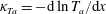
Figure 6. Frequency and growth rate of the universal mode in a contaminated pair plasma. One sees that the ion density gradient and the ion contamination must be larger than some threshold for the mode to become unstable. The ion density gradient
 $\unicode[STIX]{x1D705}_{ni}\unicode[STIX]{x1D70C}_{i}=0.3$
has been used for the
$\unicode[STIX]{x1D705}_{ni}\unicode[STIX]{x1D70C}_{i}=0.3$
has been used for the
 $\unicode[STIX]{x1D708}_{i}$
dependence (b).
$\unicode[STIX]{x1D708}_{i}$
dependence (b).
From (4.4) one sees that to be unstable at
 $\unicode[STIX]{x1D706}_{D}=0$
, the universal mode needs a finite and large enough value of
$\unicode[STIX]{x1D706}_{D}=0$
, the universal mode needs a finite and large enough value of
 $1-\unicode[STIX]{x1D6E4}_{0i}$
, which is the case if
$1-\unicode[STIX]{x1D6E4}_{0i}$
, which is the case if
 $k_{\bot }\unicode[STIX]{x1D70C}_{i}\sim 1$
. The numerical solution corresponding to this case is shown in figure 6. The dispersion relation (2.15) is solved for the parameters
$k_{\bot }\unicode[STIX]{x1D70C}_{i}\sim 1$
. The numerical solution corresponding to this case is shown in figure 6. The dispersion relation (2.15) is solved for the parameters
 $k_{\bot }\unicode[STIX]{x1D70C}_{i}=2.0$
,
$k_{\bot }\unicode[STIX]{x1D70C}_{i}=2.0$
,
 $k_{\Vert }\unicode[STIX]{x1D70C}_{i}=7.4\times 10^{-4}$
,
$k_{\Vert }\unicode[STIX]{x1D70C}_{i}=7.4\times 10^{-4}$
,
 $\unicode[STIX]{x1D705}_{Ti}=\unicode[STIX]{x1D705}_{Te}=0$
,
$\unicode[STIX]{x1D705}_{Ti}=\unicode[STIX]{x1D705}_{Te}=0$
,
 $\unicode[STIX]{x1D706}_{D}=0$
. One sees that the universal instability can exist in pair plasmas in a slab geometry but requires both the proton fraction and the ion density gradient to exceed some threshold. Note that one would have to include resonant contributions (e.g. proportional to
$\unicode[STIX]{x1D706}_{D}=0$
. One sees that the universal instability can exist in pair plasmas in a slab geometry but requires both the proton fraction and the ion density gradient to exceed some threshold. Note that one would have to include resonant contributions (e.g. proportional to
 $\text{e}^{-\unicode[STIX]{x1D701}_{i}^{2}}$
) and other higher-order terms into the growth rate calculation to find the threshold analytically. Such terms have been omitted in the derivation of (4.4), which is therefore valid only in the unstable domain. It is however straightforward to find the threshold numerically. Practically, it suggests that the universal mode will be stable in pair plasmas if the proton contamination is small. Interestingly, the positron density gradient has zero effect on the universal mode if quasineutrality
$\text{e}^{-\unicode[STIX]{x1D701}_{i}^{2}}$
) and other higher-order terms into the growth rate calculation to find the threshold analytically. Such terms have been omitted in the derivation of (4.4), which is therefore valid only in the unstable domain. It is however straightforward to find the threshold numerically. Practically, it suggests that the universal mode will be stable in pair plasmas if the proton contamination is small. Interestingly, the positron density gradient has zero effect on the universal mode if quasineutrality
 $n_{e}=n_{p}+n_{i}$
is assumed since any effect of the positron density gradient on the universal mode is perfectly cancelled by the electrons. Note, however, that the positrons still contribute through their finite fraction since
$n_{e}=n_{p}+n_{i}$
is assumed since any effect of the positron density gradient on the universal mode is perfectly cancelled by the electrons. Note, however, that the positrons still contribute through their finite fraction since
 $\unicode[STIX]{x1D708}_{i}=1-\unicode[STIX]{x1D708}_{p}$
.
$\unicode[STIX]{x1D708}_{i}=1-\unicode[STIX]{x1D708}_{p}$
.
5 ITG instability
For simplicity, we consider the flat density limit for all species. In this case, it is convenient to define
 $\unicode[STIX]{x1D714}_{Ta}=\unicode[STIX]{x1D702}_{a}\unicode[STIX]{x1D714}_{\ast a}=k_{y}T_{a}/(e_{a}B)\;\text{d}\ln T_{a}/\text{d}x$
, which is finite also at zero density gradient, with
$\unicode[STIX]{x1D714}_{Ta}=\unicode[STIX]{x1D702}_{a}\unicode[STIX]{x1D714}_{\ast a}=k_{y}T_{a}/(e_{a}B)\;\text{d}\ln T_{a}/\text{d}x$
, which is finite also at zero density gradient, with
 $a=i,e,p$
being the species index. For electrons and positrons, we also assume flat temperature profiles
$a=i,e,p$
being the species index. For electrons and positrons, we also assume flat temperature profiles
 $\unicode[STIX]{x1D714}_{Te}=\unicode[STIX]{x1D714}_{Tp}=0$
. Only for ions is the temperature gradient finite,
$\unicode[STIX]{x1D714}_{Te}=\unicode[STIX]{x1D714}_{Tp}=0$
. Only for ions is the temperature gradient finite,
 $\unicode[STIX]{x1D714}_{Ti}\neq 0$
. To allow for unequal temperatures of different species, we introduce the notation:
$\unicode[STIX]{x1D714}_{Ti}\neq 0$
. To allow for unequal temperatures of different species, we introduce the notation:
 $$\begin{eqnarray}\hat{\unicode[STIX]{x1D708}}_{a}=\frac{2\,\unicode[STIX]{x1D708}_{a}/\unicode[STIX]{x1D70F}_{a}}{\displaystyle \mathop{\sum }_{a^{\prime }}\unicode[STIX]{x1D708}_{a^{\prime }}/\unicode[STIX]{x1D70F}_{a^{\prime }}}\end{eqnarray}$$
with
 $\unicode[STIX]{x1D708}_{a}=n_{a}/n_{e}$
and
$\unicode[STIX]{x1D708}_{a}=n_{a}/n_{e}$
and
 $\unicode[STIX]{x1D70F}_{a}=T_{a}/T_{e}$
. Note that quasineutral plasmas satisfy both
$\unicode[STIX]{x1D70F}_{a}=T_{a}/T_{e}$
. Note that quasineutral plasmas satisfy both
 $\sum _{a}\unicode[STIX]{x1D708}_{a}=2$
and
$\sum _{a}\unicode[STIX]{x1D708}_{a}=2$
and
 $\sum _{a}\hat{\unicode[STIX]{x1D708}}_{a}=2$
. If the temperatures of all species are equal (
$\sum _{a}\hat{\unicode[STIX]{x1D708}}_{a}=2$
. If the temperatures of all species are equal (
 $\unicode[STIX]{x1D70F}_{a}=1$
) in such plasmas, then
$\unicode[STIX]{x1D70F}_{a}=1$
) in such plasmas, then
 $\hat{\unicode[STIX]{x1D708}_{a}}=\unicode[STIX]{x1D708}_{a}$
. Using this notation and assuming, as already mentioned, flat density profiles for all species (
$\hat{\unicode[STIX]{x1D708}_{a}}=\unicode[STIX]{x1D708}_{a}$
. Using this notation and assuming, as already mentioned, flat density profiles for all species (
 $\unicode[STIX]{x1D714}_{\ast a}=0$
), the dispersion relation becomes
$\unicode[STIX]{x1D714}_{\ast a}=0$
), the dispersion relation becomes
 $$\begin{eqnarray}1+k_{\bot }^{2}\unicode[STIX]{x1D706}_{D}^{2}+\mathop{\sum }_{a=i,p,e}\frac{\hat{\unicode[STIX]{x1D708}}_{a}}{2}\unicode[STIX]{x1D701}_{a}Z_{0a}\unicode[STIX]{x1D6E4}_{0a}+\frac{\hat{\unicode[STIX]{x1D708}}_{i}\unicode[STIX]{x1D714}_{Ti}\,\unicode[STIX]{x1D701}_{i}}{2\unicode[STIX]{x1D714}}\left(\frac{3}{2}Z_{0i}\unicode[STIX]{x1D6E4}_{0i}-Z_{0i}\unicode[STIX]{x1D6E4}_{\ast i}-Z_{2i}\unicode[STIX]{x1D6E4}_{0i}\right)=0.\end{eqnarray}$$
We consider the long-wavelength limit
 $\unicode[STIX]{x1D6E4}_{0a}=\unicode[STIX]{x1D6E4}_{\ast a}=1$
for all particle species. For the ITG instability, we can assume
$\unicode[STIX]{x1D6E4}_{0a}=\unicode[STIX]{x1D6E4}_{\ast a}=1$
for all particle species. For the ITG instability, we can assume
 $k_{\Vert }v_{\text{th}i}\ll \unicode[STIX]{x1D714}\ll k_{\Vert }v_{\text{th}e}$
. Then, the plasma dispersion function can be expanded as
$k_{\Vert }v_{\text{th}i}\ll \unicode[STIX]{x1D714}\ll k_{\Vert }v_{\text{th}e}$
. Then, the plasma dispersion function can be expanded as
 $$\begin{eqnarray}Z_{0}(\unicode[STIX]{x1D701}_{i})\approx -\frac{1}{\unicode[STIX]{x1D701}_{i}}-\frac{1}{2\unicode[STIX]{x1D701}_{i}^{3}}-\frac{3}{4\unicode[STIX]{x1D701}_{i}^{5}},\quad Z_{0}(\unicode[STIX]{x1D701}_{p})=Z_{0}(\unicode[STIX]{x1D701}_{e})\approx \text{i}\sqrt{\unicode[STIX]{x03C0}}.\end{eqnarray}$$
Using (2.12), it is straightforward to derive
 $Z_{2i}=\unicode[STIX]{x1D701}_{i}(1+\unicode[STIX]{x1D701}_{i}Z_{0i})$
. Here, one sees that the fifth-order term must be included into the expansion of
$Z_{2i}=\unicode[STIX]{x1D701}_{i}(1+\unicode[STIX]{x1D701}_{i}Z_{0i})$
. Here, one sees that the fifth-order term must be included into the expansion of
 $Z_{0i}$
appearing in
$Z_{0i}$
appearing in
 $Z_{2i}$
since we need cubic (
$Z_{2i}$
since we need cubic (
 ${\sim}1/\unicode[STIX]{x1D701}_{i}^{3}$
) terms for the ITG instability and we must keep all of them for consistency. Neglecting ion FLR effects (i.e. setting
${\sim}1/\unicode[STIX]{x1D701}_{i}^{3}$
) terms for the ITG instability and we must keep all of them for consistency. Neglecting ion FLR effects (i.e. setting
 $\unicode[STIX]{x1D6E4}_{0i}=1$
and
$\unicode[STIX]{x1D6E4}_{0i}=1$
and
 $\unicode[STIX]{x1D6E4}_{\ast i}=1$
) as well as the electron and positron contributions (
$\unicode[STIX]{x1D6E4}_{\ast i}=1$
) as well as the electron and positron contributions (
 ${\sim}\unicode[STIX]{x1D701}_{e}\ll 1$
), we obtain to leading order in
${\sim}\unicode[STIX]{x1D701}_{e}\ll 1$
), we obtain to leading order in
 $1/\unicode[STIX]{x1D701}_{i}$
 $$\begin{eqnarray}1-\frac{\hat{\unicode[STIX]{x1D708}}_{i}}{2}+k_{\bot }^{2}\unicode[STIX]{x1D706}_{D}^{2}=-\frac{\hat{\unicode[STIX]{x1D708}}_{i}\unicode[STIX]{x1D714}_{Ti}}{4\unicode[STIX]{x1D714}\unicode[STIX]{x1D701}_{i}^{2}}+\frac{\unicode[STIX]{x1D708}_{i}}{2\unicode[STIX]{x1D701}_{i}^{2}}.\end{eqnarray}$$
Following Coppi, Rosenbluth & Sagdeev (Reference Coppi, Rosenbluth and Sagdeev1967), we also assume
 $\unicode[STIX]{x1D714}_{Ti}\gg \unicode[STIX]{x1D714}$
. Then
$\unicode[STIX]{x1D714}_{Ti}\gg \unicode[STIX]{x1D714}$
. Then
 $$\begin{eqnarray}1-\frac{\hat{\unicode[STIX]{x1D708}}_{i}}{2}+k_{\bot }^{2}\unicode[STIX]{x1D706}_{D}^{2}=-\frac{\hat{\unicode[STIX]{x1D708}}_{i}\unicode[STIX]{x1D714}_{Ti}}{4\unicode[STIX]{x1D714}^{3}}k_{\Vert }^{2}v_{\text{th}i}^{2}.\end{eqnarray}$$
Note that by definition
 $\unicode[STIX]{x1D714}_{Ti}=\unicode[STIX]{x1D702}_{i}\unicode[STIX]{x1D714}_{\ast i}$
with
$\unicode[STIX]{x1D714}_{Ti}=\unicode[STIX]{x1D702}_{i}\unicode[STIX]{x1D714}_{\ast i}$
with
 $\unicode[STIX]{x1D714}_{\ast i}<0$
, see § 2, and
$\unicode[STIX]{x1D714}_{\ast i}<0$
, see § 2, and
 $\unicode[STIX]{x1D702}_{i}>0$
. Hence,
$\unicode[STIX]{x1D702}_{i}>0$
. Hence,
 $\unicode[STIX]{x1D714}_{Ti}<0$
and there is an unstable solution of the dispersion relation (5.5):
$\unicode[STIX]{x1D714}_{Ti}<0$
and there is an unstable solution of the dispersion relation (5.5):
 $$\begin{eqnarray}\unicode[STIX]{x1D714}=\frac{1}{2^{1/3}}\left(\frac{\hat{\unicode[STIX]{x1D708}}_{i}|\unicode[STIX]{x1D714}_{Ti}|k_{\Vert }^{2}v_{\text{th}i}^{2}}{2-\hat{\unicode[STIX]{x1D708}}_{i}+2k_{\bot }^{2}\unicode[STIX]{x1D706}_{D}^{2}}\right)^{1/3}\left(-\frac{1}{2}+\text{i}\frac{\sqrt{3}}{2}\right).\end{eqnarray}$$
This root corresponds to the well-known fluid limit of the slab ITG instability (Coppi et al.
Reference Coppi, Rosenbluth and Sagdeev1967). Note that the real part of the ITG frequency is negative, as expected. One sees that in an ion-contaminated electron–positron plasma, the frequency and growth rate of the fluid ITG instability are proportional to
 $(\hat{\unicode[STIX]{x1D708}}_{i}|\unicode[STIX]{x1D714}_{Ti}|)^{1/3}$
. Hence, pure pair plasmas with
$(\hat{\unicode[STIX]{x1D708}}_{i}|\unicode[STIX]{x1D714}_{Ti}|)^{1/3}$
. Hence, pure pair plasmas with
 $\hat{\unicode[STIX]{x1D708}}_{i}=0$
cannot support the slab ITG. This is an obvious conclusion since the absence of ions guarantees the absence of ion-temperature-gradient-driven instabilities. More important, however, is that, similarly to the frequency and the growth rate, the destabilisation threshold is also determined by the product
$\hat{\unicode[STIX]{x1D708}}_{i}=0$
cannot support the slab ITG. This is an obvious conclusion since the absence of ions guarantees the absence of ion-temperature-gradient-driven instabilities. More important, however, is that, similarly to the frequency and the growth rate, the destabilisation threshold is also determined by the product
 $\hat{\unicode[STIX]{x1D708}}_{i}|\unicode[STIX]{x1D714}_{Ti}|$
, and not just
$\hat{\unicode[STIX]{x1D708}}_{i}|\unicode[STIX]{x1D714}_{Ti}|$
, and not just
 $|\unicode[STIX]{x1D714}_{Ti}|$
as is the case for conventional (e.g. hydrogen) plasmas. This can be deduced from the fact that
$|\unicode[STIX]{x1D714}_{Ti}|$
as is the case for conventional (e.g. hydrogen) plasmas. This can be deduced from the fact that
 $\unicode[STIX]{x1D714}_{Ti}$
appears only in combination with
$\unicode[STIX]{x1D714}_{Ti}$
appears only in combination with
 $\unicode[STIX]{x1D708}_{i}$
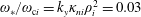
in the original dispersion relation, equation (5.2). Note that the solution equation (5.6) corresponds to the fluid instability and does not contain information about the threshold. In this paper, we do not derive the threshold analytically, but we can easily find it numerically. Numerical results demonstrating this prediction are shown in figure 7. Here, the dependence of the ITG frequency and the growth rate on the proton contamination is plotted. One sees that the absolute value of the frequency indeed decreases strongly at a smaller proton content, in agreement with the analytic result. One also sees that the mode is unstable only when the proton content exceeds some threshold, whose value depends on the ion temperature gradient. This is of practical interest since it indicates that the ITG modes may be stable at a large ion temperature gradient in ion-contaminated pair plasmas if the ion fraction is small enough. Other parameters, such as the density gradient or wavenumbers, can affect the value of the threshold, too, but we keep all other parameters fixed in the calculation shown in figure 7, changing only the proton fraction for two different values of the ion temperature gradient.
$\unicode[STIX]{x1D708}_{i}$
in the original dispersion relation, equation (5.2). Note that the solution equation (5.6) corresponds to the fluid instability and does not contain information about the threshold. In this paper, we do not derive the threshold analytically, but we can easily find it numerically. Numerical results demonstrating this prediction are shown in figure 7. Here, the dependence of the ITG frequency and the growth rate on the proton contamination is plotted. One sees that the absolute value of the frequency indeed decreases strongly at a smaller proton content, in agreement with the analytic result. One also sees that the mode is unstable only when the proton content exceeds some threshold, whose value depends on the ion temperature gradient. This is of practical interest since it indicates that the ITG modes may be stable at a large ion temperature gradient in ion-contaminated pair plasmas if the ion fraction is small enough. Other parameters, such as the density gradient or wavenumbers, can affect the value of the threshold, too, but we keep all other parameters fixed in the calculation shown in figure 7, changing only the proton fraction for two different values of the ion temperature gradient.

Figure 7. Effect of proton contamination on the ITG mode in a pair plasma. The wavenumbers are
 $k_{\bot }\unicode[STIX]{x1D70C}_{i}=0.24$
and
$k_{\bot }\unicode[STIX]{x1D70C}_{i}=0.24$
and
 $k_{\Vert }\unicode[STIX]{x1D70C}_{i}=7.4\times 10^{-4}$
. The density and the electron temperature profiles are flat,
$k_{\Vert }\unicode[STIX]{x1D70C}_{i}=7.4\times 10^{-4}$
. The density and the electron temperature profiles are flat,
 $\unicode[STIX]{x1D705}_{\text{T}i}=-\text{d}\ln T_{i}(x)/\text{d}x$
, and
$\unicode[STIX]{x1D705}_{\text{T}i}=-\text{d}\ln T_{i}(x)/\text{d}x$
, and
 $\unicode[STIX]{x1D70F}_{i}=1$
.
$\unicode[STIX]{x1D70F}_{i}=1$
.

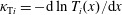
Figure 8. ITG mode in a pair plasma with the proton contamination
 $\unicode[STIX]{x1D708}_{i}=0.13$
for
$\unicode[STIX]{x1D708}_{i}=0.13$
for
 $\unicode[STIX]{x1D70F}_{i}=1$
and
$\unicode[STIX]{x1D70F}_{i}=1$
and
 $k_{\Vert }\unicode[STIX]{x1D70C}_{i}=7.4\times 10^{-4}$
. Effect of the finite Debye length is considered.
$k_{\Vert }\unicode[STIX]{x1D70C}_{i}=7.4\times 10^{-4}$
. Effect of the finite Debye length is considered.
Another aspect of practical interest for the pair-plasma experiment (Pedersen et al.
Reference Pedersen, Danielson, Hugenschmidt, Marx, Sarasola, Schauer, Schweikhard, Surko and Winkler2012) is the effect of the Debye length on the microinstabilities. This effect is usually negligible for tokamak or stellarator plasmas, where the Debye length is much smaller than the ion gyroradius. In the pair-plasma experiment, however, the Debye length is not expected to be very small and can become comparable to the proton gyroradius. This can have a strongly stabilising effect on the ITG stability, as shown in figure 8. One sees that for a given
 $k_{\Vert }$
, the ITG instability can disappear for all perpendicular wavelengths if
$k_{\Vert }$
, the ITG instability can disappear for all perpendicular wavelengths if
 $\unicode[STIX]{x1D706}_{D}/\unicode[STIX]{x1D70C}_{i}$
is large enough.
$\unicode[STIX]{x1D706}_{D}/\unicode[STIX]{x1D70C}_{i}$
is large enough.
6 ETG instability
Consider now the case when only electron and positron temperature gradients are present, i.e.
 $\unicode[STIX]{x1D714}_{T(e,p)}\neq 0$
, while
$\unicode[STIX]{x1D714}_{T(e,p)}\neq 0$
, while
 $\unicode[STIX]{x1D714}_{Ti}=0$
and
$\unicode[STIX]{x1D714}_{Ti}=0$
and
 $\unicode[STIX]{x1D714}_{\ast (e,p,i)}=0$
(flat density). Recall that
$\unicode[STIX]{x1D714}_{\ast (e,p,i)}=0$
(flat density). Recall that
 $\unicode[STIX]{x1D714}_{Ta}=k_{y}T_{a}/(e_{a}B)\;\text{d}\ln T_{a}/\text{d}x$
is proportional to the temperature gradient and can be finite also at
$\unicode[STIX]{x1D714}_{Ta}=k_{y}T_{a}/(e_{a}B)\;\text{d}\ln T_{a}/\text{d}x$
is proportional to the temperature gradient and can be finite also at
 $\unicode[STIX]{x1D714}_{\ast a}=0$
. In this section, we will also allow for unequal temperatures of different species. Therefore, the notation defined in (5.1) will be used. For the perpendicular wavenumbers, we assume
$\unicode[STIX]{x1D714}_{\ast a}=0$
. In this section, we will also allow for unequal temperatures of different species. Therefore, the notation defined in (5.1) will be used. For the perpendicular wavenumbers, we assume
 $k_{\bot }\unicode[STIX]{x1D70C}_{i}\gg 1$
implying
$k_{\bot }\unicode[STIX]{x1D70C}_{i}\gg 1$
implying
 $\unicode[STIX]{x1D6E4}_{0i}=0$
and
$\unicode[STIX]{x1D6E4}_{0i}=0$
and
 $\unicode[STIX]{x1D6E4}_{\ast i}=0$
. In this limit, the dispersion relation is
$\unicode[STIX]{x1D6E4}_{\ast i}=0$
. In this limit, the dispersion relation is
 $$\begin{eqnarray}1+k_{\bot }^{2}\unicode[STIX]{x1D706}_{D}^{2}+\mathop{\sum }_{a=p,e}\frac{\hat{\unicode[STIX]{x1D708}}_{a}}{2}\unicode[STIX]{x1D701}_{a}\left[Z_{0a}\unicode[STIX]{x1D6E4}_{0a}+\frac{\unicode[STIX]{x1D714}_{Ta}}{\unicode[STIX]{x1D714}}\left(\frac{3}{2}Z_{0a}\unicode[STIX]{x1D6E4}_{0a}-Z_{0a}\unicode[STIX]{x1D6E4}_{\ast a}-Z_{2a}\unicode[STIX]{x1D6E4}_{0a}\right)\right]=0.\end{eqnarray}$$
Here, recall that from (2.12) one can derive
 $Z_{2a}=\unicode[STIX]{x1D701}_{a}(1+\unicode[STIX]{x1D701}_{a}Z_{0a})$
. Assuming large frequencies
$Z_{2a}=\unicode[STIX]{x1D701}_{a}(1+\unicode[STIX]{x1D701}_{a}Z_{0a})$
. Assuming large frequencies
 $\unicode[STIX]{x1D714}\gg k_{\Vert }v_{\text{th}(e,p)}$
, we can write
$\unicode[STIX]{x1D714}\gg k_{\Vert }v_{\text{th}(e,p)}$
, we can write
 $$\begin{eqnarray}Z_{0}(\unicode[STIX]{x1D701}_{e,p})\approx -\frac{1}{\unicode[STIX]{x1D701}_{e,p}}-\frac{1}{2\unicode[STIX]{x1D701}_{e,p}^{3}}-\frac{3}{4\unicode[STIX]{x1D701}_{e,p}^{5}}.\end{eqnarray}$$
The fifth-order term in this expansion is needed to account for the quadratic (
 ${\sim}\unicode[STIX]{x1D701}_{a}^{2}$
) contribution appearing in
${\sim}\unicode[STIX]{x1D701}_{a}^{2}$
) contribution appearing in
 $Z_{2a}$
. Assuming in addition small
$Z_{2a}$
. Assuming in addition small
 $k_{\bot }\unicode[STIX]{x1D70C}_{(e,p)}\ll 1$
, i.e.
$k_{\bot }\unicode[STIX]{x1D70C}_{(e,p)}\ll 1$
, i.e.
 $\unicode[STIX]{x1D6E4}_{0(e,p)}=1$
and
$\unicode[STIX]{x1D6E4}_{0(e,p)}=1$
and
 $\unicode[STIX]{x1D6E4}_{\ast (e,p)}=1$
, we finally obtain to the leading order
$\unicode[STIX]{x1D6E4}_{\ast (e,p)}=1$
, we finally obtain to the leading order
 $$\begin{eqnarray}\displaystyle \left(\frac{\hat{\unicode[STIX]{x1D708}}_{i}}{2}+k_{\bot }^{2}\unicode[STIX]{x1D706}_{D}^{2}\right)+\frac{\hat{\unicode[STIX]{x1D708}}_{e}\unicode[STIX]{x1D70F}_{e}\unicode[STIX]{x1D714}_{Te}+\hat{\unicode[STIX]{x1D708}}_{p}\unicode[STIX]{x1D70F}_{p}\unicode[STIX]{x1D714}_{Tp}}{4\unicode[STIX]{x1D714}\unicode[STIX]{x1D701}_{e}^{2}}=0. & & \displaystyle\end{eqnarray}$$
Here, the relations
 $\sum _{a}\hat{\unicode[STIX]{x1D708}}_{a}=2$
and
$\sum _{a}\hat{\unicode[STIX]{x1D708}}_{a}=2$
and
 $\unicode[STIX]{x1D701}_{p}^{2}=\unicode[STIX]{x1D701}_{e}^{2}/\unicode[STIX]{x1D70F}_{p}$
have been employed. Similarly to the ITG derivation, equation (5.5), we have assumed
$\unicode[STIX]{x1D701}_{p}^{2}=\unicode[STIX]{x1D701}_{e}^{2}/\unicode[STIX]{x1D70F}_{p}$
have been employed. Similarly to the ITG derivation, equation (5.5), we have assumed
 $\unicode[STIX]{x1D714}_{Te}\sim \unicode[STIX]{x1D714}_{Tp}\gg \unicode[STIX]{x1D714}$
, following Coppi et al. (Reference Coppi, Rosenbluth and Sagdeev1967), i.e. our derivation of (6.3) follows exactly the same path as in the ITG case, equation (5.5).
$\unicode[STIX]{x1D714}_{Te}\sim \unicode[STIX]{x1D714}_{Tp}\gg \unicode[STIX]{x1D714}$
, following Coppi et al. (Reference Coppi, Rosenbluth and Sagdeev1967), i.e. our derivation of (6.3) follows exactly the same path as in the ITG case, equation (5.5).
Let us now consider the case of equal electron and positron temperature profiles, implying
 $\unicode[STIX]{x1D70F}_{p}=\unicode[STIX]{x1D70F}_{e}=1$
and
$\unicode[STIX]{x1D70F}_{p}=\unicode[STIX]{x1D70F}_{e}=1$
and
 $\unicode[STIX]{x1D714}_{Te}+\unicode[STIX]{x1D714}_{Tp}=0$
. Recall that
$\unicode[STIX]{x1D714}_{Te}+\unicode[STIX]{x1D714}_{Tp}=0$
. Recall that
 $\unicode[STIX]{x1D70F}_{a}=T_{a}/T_{e}$
, and our sign conventions imply
$\unicode[STIX]{x1D70F}_{a}=T_{a}/T_{e}$
, and our sign conventions imply
 $\unicode[STIX]{x1D714}_{Te}>0$
and
$\unicode[STIX]{x1D714}_{Te}>0$
and
 $\unicode[STIX]{x1D714}_{Tp}<0$
. These conditions are likely since the characteristic time of the energy exchange between the electrons and the positrons is comparable to their Maxwellisation time. If the plasma has had time to reach a locally Maxwellian state, as we have assumed, the electron and positron temperatures should also have equilibrated. In contrast, the ion temperature can differ from the electron one, implying
$\unicode[STIX]{x1D714}_{Tp}<0$
. These conditions are likely since the characteristic time of the energy exchange between the electrons and the positrons is comparable to their Maxwellisation time. If the plasma has had time to reach a locally Maxwellian state, as we have assumed, the electron and positron temperatures should also have equilibrated. In contrast, the ion temperature can differ from the electron one, implying
 $\unicode[STIX]{x1D70F}_{i}\neq 1$
. Then, the unstable solution is
$\unicode[STIX]{x1D70F}_{i}\neq 1$
. Then, the unstable solution is
 $$\begin{eqnarray}\unicode[STIX]{x1D714}=\frac{1}{2^{1/3}}\left(\frac{k_{\Vert }^{2}v_{\text{th}e}^{2}}{\hat{\unicode[STIX]{x1D708}_{i}}+2k_{\bot }^{2}\unicode[STIX]{x1D706}_{D}^{2}}\;\hat{\unicode[STIX]{x1D708}}_{i}\unicode[STIX]{x1D70F}_{i}\unicode[STIX]{x1D714}_{Te}\right)^{1/3}\left(\frac{1}{2}+\text{i}\,\frac{\sqrt{3}}{2}\right).\end{eqnarray}$$
This solution corresponds to the fluid limit of the slab ETG instability, which is similar to the ITG instability, equation (5.6), but has a frequency of the opposite sign. The mode is expected to be stable in a pure pair plasma
 $\hat{\unicode[STIX]{x1D708}_{i}}=0$
, as can indeed be seen from the numerical solution of the full dispersion relation (2.15), shown in figure 9. In (6.4), however, also the denominator vanishes at
$\hat{\unicode[STIX]{x1D708}_{i}}=0$
, as can indeed be seen from the numerical solution of the full dispersion relation (2.15), shown in figure 9. In (6.4), however, also the denominator vanishes at
 $\hat{\unicode[STIX]{x1D708}_{i}}=0$
if
$\hat{\unicode[STIX]{x1D708}_{i}}=0$
if
 $k_{\bot }\unicode[STIX]{x1D706}_{D}=0$
. This singular limit contradicts to the assumption
$k_{\bot }\unicode[STIX]{x1D706}_{D}=0$
. This singular limit contradicts to the assumption
 $\unicode[STIX]{x1D714}\ll \unicode[STIX]{x1D714}_{Te}$
made in the derivation of (6.4). Therefore this equation cannot be used at very small
$\unicode[STIX]{x1D714}\ll \unicode[STIX]{x1D714}_{Te}$
made in the derivation of (6.4). Therefore this equation cannot be used at very small
 $\unicode[STIX]{x1D708}_{i}$
unless
$\unicode[STIX]{x1D708}_{i}$
unless
 $k_{\bot }\unicode[STIX]{x1D706}_{D}$
is finite. For finite
$k_{\bot }\unicode[STIX]{x1D706}_{D}$
is finite. For finite
 $k_{\bot }\unicode[STIX]{x1D706}_{D}$
, there is no singularity and (6.4) is valid even at very small
$k_{\bot }\unicode[STIX]{x1D706}_{D}$
, there is no singularity and (6.4) is valid even at very small
 $\unicode[STIX]{x1D708}_{i}$
. For this regime, however, the finite Debye length effects are important. For example,
$\unicode[STIX]{x1D708}_{i}$
. For this regime, however, the finite Debye length effects are important. For example,
 $\unicode[STIX]{x1D714}$
is proportional to
$\unicode[STIX]{x1D714}$
is proportional to
 $(k_{\bot }\unicode[STIX]{x1D706}_{D})^{-2/3}$
if
$(k_{\bot }\unicode[STIX]{x1D706}_{D})^{-2/3}$
if
 $\unicode[STIX]{x1D708}_{i}\ll k_{\bot }^{2}\unicode[STIX]{x1D706}_{D}^{2}$
.
$\unicode[STIX]{x1D708}_{i}\ll k_{\bot }^{2}\unicode[STIX]{x1D706}_{D}^{2}$
.

Figure 9. Frequency and growth rate of the ETG mode in a three-component electron–positron-proton plasma for
 $\unicode[STIX]{x1D714}_{Tp}=\unicode[STIX]{x1D714}_{Te}$
. One sees that the ion fraction must exceed some threshold for the ETG to be unstable. Here,
$\unicode[STIX]{x1D714}_{Tp}=\unicode[STIX]{x1D714}_{Te}$
. One sees that the ion fraction must exceed some threshold for the ETG to be unstable. Here,
 $k_{\Vert }\unicode[STIX]{x1D70C}_{i}=7.4\times 10^{-4}$
,
$k_{\Vert }\unicode[STIX]{x1D70C}_{i}=7.4\times 10^{-4}$
,
 $\unicode[STIX]{x1D705}_{\text{n}i}=\unicode[STIX]{x1D705}_{\text{n}e}=\unicode[STIX]{x1D705}_{\text{n}p}=0$
,
$\unicode[STIX]{x1D705}_{\text{n}i}=\unicode[STIX]{x1D705}_{\text{n}e}=\unicode[STIX]{x1D705}_{\text{n}p}=0$
,
 $\unicode[STIX]{x1D705}_{\text{T}i}=0$
,
$\unicode[STIX]{x1D705}_{\text{T}i}=0$
,
 $\unicode[STIX]{x1D705}_{\text{T}e}\unicode[STIX]{x1D70C}_{i}=\unicode[STIX]{x1D705}_{\text{T}p}\unicode[STIX]{x1D70C}_{i}=0.1$
,
$\unicode[STIX]{x1D705}_{\text{T}e}\unicode[STIX]{x1D70C}_{i}=\unicode[STIX]{x1D705}_{\text{T}p}\unicode[STIX]{x1D70C}_{i}=0.1$
,
 $\unicode[STIX]{x1D706}_{D}=0$
and
$\unicode[STIX]{x1D706}_{D}=0$
and
 $\unicode[STIX]{x1D70F}_{a}=1$
with
$\unicode[STIX]{x1D70F}_{a}=1$
with
 $a=(i,e,p)$
.
$a=(i,e,p)$
.
Now, we consider a situation in which the electron and the positron temperature gradients are different for some reason, implying
 $\unicode[STIX]{x1D714}_{Te}+\unicode[STIX]{x1D714}_{Tp}\neq 0$
. In this case, one can show that the ETG mode can be unstable also in a pure pair plasma (
$\unicode[STIX]{x1D714}_{Te}+\unicode[STIX]{x1D714}_{Tp}\neq 0$
. In this case, one can show that the ETG mode can be unstable also in a pure pair plasma (
 $\hat{\unicode[STIX]{x1D708}}_{i}=0$
). Assuming for simplicity
$\hat{\unicode[STIX]{x1D708}}_{i}=0$
). Assuming for simplicity
 $k_{\bot }\unicode[STIX]{x1D706}_{D}$
to be finite, we can write the unstable ETG solution as
$k_{\bot }\unicode[STIX]{x1D706}_{D}$
to be finite, we can write the unstable ETG solution as
 $$\begin{eqnarray}\unicode[STIX]{x1D714}=\frac{1}{2^{1/3}}\left(\frac{k_{\Vert }^{2}v_{\text{th}e}^{2}}{k_{\bot }^{2}\unicode[STIX]{x1D706}_{D}^{2}}\,\frac{\unicode[STIX]{x1D70F}_{e}\unicode[STIX]{x1D70F}_{p}}{\unicode[STIX]{x1D70F}_{e}+\unicode[STIX]{x1D70F}_{p}}\;[|\unicode[STIX]{x1D714}_{Te}|-|\unicode[STIX]{x1D714}_{Tp}|]\right)^{1/3}\left(\frac{1}{2}+\text{i}\,\frac{\sqrt{3}}{2}\right).\end{eqnarray}$$
The numerical solution of the dispersion relation (2.15) corresponding to a pure pair-plasma ETG is shown in figure 10. This result is valid if the electrons have a steeper temperature profile. Otherwise, the ETG instability is replaced by the positron-temperature-gradient (PTG) driven instability, which has a negative frequency:
 $$\begin{eqnarray}\unicode[STIX]{x1D714}=\frac{1}{2^{1/3}}\left(\frac{k_{\Vert }^{2}v_{\text{th}e}^{2}}{k_{\bot }^{2}\unicode[STIX]{x1D706}_{D}^{2}}\,\frac{\unicode[STIX]{x1D70F}_{e}\unicode[STIX]{x1D70F}_{p}}{\unicode[STIX]{x1D70F}_{e}+\unicode[STIX]{x1D70F}_{p}}[|\unicode[STIX]{x1D714}_{Tp}|-|\unicode[STIX]{x1D714}_{Te}|]\right)^{1/3}\left(-\frac{1}{2}+\text{i}\frac{\sqrt{3}}{2}\right).\end{eqnarray}$$
The PTG solution is shown in figure 11. One can see that the frequency of the PTG instability is negative whereas the frequency of the ETG instability, figure 10, is positive, as suggested by (6.5) and (6.6). The growth rates of both instabilities are equal. The absolute values of the ETG and PTG frequencies are equal, too, in agreement with (6.5) and (6.6). Finally, one can see that the growth rate increases with
 $|\unicode[STIX]{x1D714}_{Te}+\unicode[STIX]{x1D714}_{Tp}|$
for both instabilities. The modes are stable when
$|\unicode[STIX]{x1D714}_{Te}+\unicode[STIX]{x1D714}_{Tp}|$
for both instabilities. The modes are stable when
 $|\unicode[STIX]{x1D714}_{Te}+\unicode[STIX]{x1D714}_{Tp}|=0$
, as expected. Note that
$|\unicode[STIX]{x1D714}_{Te}+\unicode[STIX]{x1D714}_{Tp}|=0$
, as expected. Note that
 $\unicode[STIX]{x1D714}_{Te}/\unicode[STIX]{x1D714}_{\text{c}i}=k_{y}\unicode[STIX]{x1D705}_{Te}\unicode[STIX]{x1D70C}_{i}^{2}$
and
$\unicode[STIX]{x1D714}_{Te}/\unicode[STIX]{x1D714}_{\text{c}i}=k_{y}\unicode[STIX]{x1D705}_{Te}\unicode[STIX]{x1D70C}_{i}^{2}$
and
 $\unicode[STIX]{x1D714}_{Tp}/\unicode[STIX]{x1D714}_{\text{c}i}=-k_{y}\unicode[STIX]{x1D705}_{Tp}\unicode[STIX]{x1D70C}_{i}^{2}$
, so that
$\unicode[STIX]{x1D714}_{Tp}/\unicode[STIX]{x1D714}_{\text{c}i}=-k_{y}\unicode[STIX]{x1D705}_{Tp}\unicode[STIX]{x1D70C}_{i}^{2}$
, so that
 $\unicode[STIX]{x1D714}_{Te}+\unicode[STIX]{x1D714}_{Tp}$
is proportional to
$\unicode[STIX]{x1D714}_{Te}+\unicode[STIX]{x1D714}_{Tp}$
is proportional to
 $\unicode[STIX]{x1D705}_{Te}-\unicode[STIX]{x1D705}_{Tp}$
. Here, the ion gyroradius
$\unicode[STIX]{x1D705}_{Te}-\unicode[STIX]{x1D705}_{Tp}$
. Here, the ion gyroradius
 $\unicode[STIX]{x1D70C}_{i}=\sqrt{m_{H}T_{e}}/(eB)$
with
$\unicode[STIX]{x1D70C}_{i}=\sqrt{m_{H}T_{e}}/(eB)$
with
 $m_{H}$
the proton mass is defined through the electron temperature and used as a normalisation constant in pure pair plasma, which does not contain ions by definition.
$m_{H}$
the proton mass is defined through the electron temperature and used as a normalisation constant in pure pair plasma, which does not contain ions by definition.

Figure 10. Frequency and growth rate of the ETG mode in a pure pair plasma when the symmetry between the species is broken by a difference in the electron and positron temperature profiles. The electron temperature profile with
 $\unicode[STIX]{x1D705}_{\text{T}e}\unicode[STIX]{x1D70C}_{i}=0.1$
is kept fixed. Here,
$\unicode[STIX]{x1D705}_{\text{T}e}\unicode[STIX]{x1D70C}_{i}=0.1$
is kept fixed. Here,
 $\unicode[STIX]{x1D706}_{D}/\unicode[STIX]{x1D70C}_{i}=0.1$
and
$\unicode[STIX]{x1D706}_{D}/\unicode[STIX]{x1D70C}_{i}=0.1$
and
 $\unicode[STIX]{x1D70F}_{a}=1$
with
$\unicode[STIX]{x1D70F}_{a}=1$
with
 $a=(e,p)$
. Note that
$a=(e,p)$
. Note that
 $\unicode[STIX]{x1D70C}_{i}=\sqrt{m_{H}T_{e}}/(eB)$
with
$\unicode[STIX]{x1D70C}_{i}=\sqrt{m_{H}T_{e}}/(eB)$
with
 $m_{H}$
the proton mass is used here as a normalisation constant since pure pair plasmas do not contain ions.
$m_{H}$
the proton mass is used here as a normalisation constant since pure pair plasmas do not contain ions.
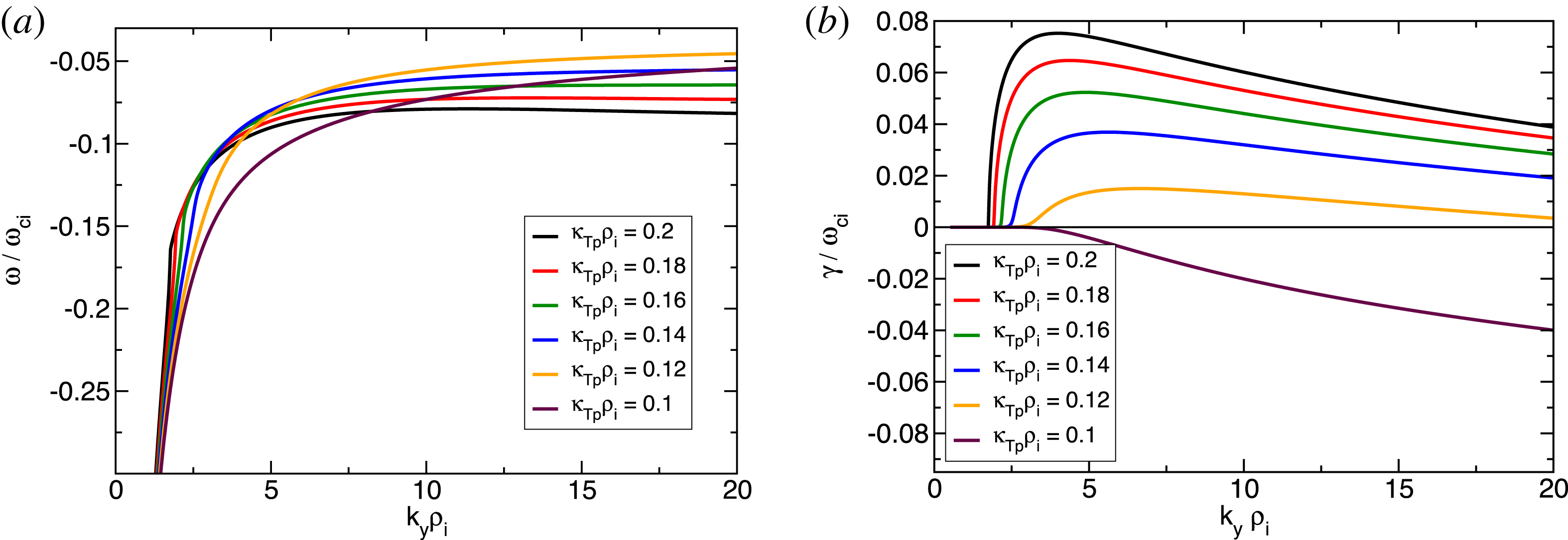
Figure 11. Frequency and growth rate of the positron-temperature-gradient mode in a pure pair plasma when the symmetry between the species is broken by a difference in the electron and positron temperature profiles. The electron temperature profile with
 $\unicode[STIX]{x1D705}_{\text{T}e}\unicode[STIX]{x1D70C}_{i}=0.1$
is kept fixed. Here,
$\unicode[STIX]{x1D705}_{\text{T}e}\unicode[STIX]{x1D70C}_{i}=0.1$
is kept fixed. Here,
 $\unicode[STIX]{x1D706}_{D}/\unicode[STIX]{x1D70C}_{i}=0.1$
and
$\unicode[STIX]{x1D706}_{D}/\unicode[STIX]{x1D70C}_{i}=0.1$
and
 $\unicode[STIX]{x1D70F}_{a}=1$
with
$\unicode[STIX]{x1D70F}_{a}=1$
with
 $a=(e,p)$
. Note that
$a=(e,p)$
. Note that
 $\unicode[STIX]{x1D70C}_{i}=\sqrt{m_{H}T_{e}}/(eB)$
with
$\unicode[STIX]{x1D70C}_{i}=\sqrt{m_{H}T_{e}}/(eB)$
with
 $m_{H}$
the proton mass is used here as a normalisation constant since pure pair plasmas do not contain ions.
$m_{H}$
the proton mass is used here as a normalisation constant since pure pair plasmas do not contain ions.
7 Shear Alfvén wave
Finally, we consider a homogeneous plasma (all profiles are flat) and solve the electromagnetic dispersion relation (2.15) at finite
 $\unicode[STIX]{x1D6FD}$
. In this case, there are no sources of free energy and, hence, no instabilities (all modes are damped or marginal). From the definition of the plasma dispersion function, equation (2.12), one can derive
$\unicode[STIX]{x1D6FD}$
. In this case, there are no sources of free energy and, hence, no instabilities (all modes are damped or marginal). From the definition of the plasma dispersion function, equation (2.12), one can derive
 $Z_{1a}=1+\unicode[STIX]{x1D701}_{a}Z_{0a}$
and
$Z_{1a}=1+\unicode[STIX]{x1D701}_{a}Z_{0a}$
and
 $Z_{2a}=\unicode[STIX]{x1D701}_{a}Z_{1a}$
. Assuming
$Z_{2a}=\unicode[STIX]{x1D701}_{a}Z_{1a}$
. Assuming
 $k_{\Vert }v_{\text{th}i}\ll \unicode[STIX]{x1D714}\ll k_{\Vert }v_{\text{th}e}$
, one can thus write:
$k_{\Vert }v_{\text{th}i}\ll \unicode[STIX]{x1D714}\ll k_{\Vert }v_{\text{th}e}$
, one can thus write:
 $$\begin{eqnarray}\displaystyle & & \displaystyle Z_{0i}=-\frac{1}{\unicode[STIX]{x1D701}_{i}}-\frac{1}{2\unicode[STIX]{x1D701}_{i}^{3}}+O\left(\frac{1}{\unicode[STIX]{x1D701}_{i}^{5}}\right),\quad Z_{0(e,p)}=\text{i}\sqrt{\unicode[STIX]{x03C0}}+O(\unicode[STIX]{x1D701}_{e})\end{eqnarray}$$
 $$\begin{eqnarray}\displaystyle & & \displaystyle Z_{1i}=-\frac{1}{2\unicode[STIX]{x1D701}_{i}^{2}}+O\left(\frac{1}{\unicode[STIX]{x1D701}_{i}^{4}}\right),\quad Z_{1(e,p)}=1+O(\unicode[STIX]{x1D701}_{e})\end{eqnarray}$$
 $$\begin{eqnarray}\displaystyle & & \displaystyle Z_{2i}=-\frac{1}{2\unicode[STIX]{x1D701}_{i}}+O\left(\frac{1}{\unicode[STIX]{x1D701}_{i}^{3}}\right),\quad Z_{2(e,p)}=\unicode[STIX]{x1D701}_{e}+O(\unicode[STIX]{x1D701}_{e}^{2}).\end{eqnarray}$$
For flat profiles
 $\unicode[STIX]{x1D714}_{\ast a}=0$
and
$\unicode[STIX]{x1D714}_{\ast a}=0$
and
 $\unicode[STIX]{x1D702}_{a}=0$
. Hence, from (2.9)
$\unicode[STIX]{x1D702}_{a}=0$
. Hence, from (2.9)
 $$\begin{eqnarray}W_{0a}=\unicode[STIX]{x1D701}_{a}Z_{0a}\unicode[STIX]{x1D6E4}_{0a},\quad W_{1a}=\unicode[STIX]{x1D701}_{a}Z_{1a}\unicode[STIX]{x1D6E4}_{0a},\quad W_{2a}=\unicode[STIX]{x1D701}_{a}Z_{2a}\unicode[STIX]{x1D6E4}_{0a}.\end{eqnarray}$$
We consider perpendicular scales much larger than the electron gyroradius so that one can neglect electron and positron FLR effects, implying
 $\unicode[STIX]{x1D6E4}_{0e}=1$
and
$\unicode[STIX]{x1D6E4}_{0e}=1$
and
 $\unicode[STIX]{x1D6E4}_{0p}=1$
. Employing the appropriate expansions of the plasma dispersion function, we obtain:
$\unicode[STIX]{x1D6E4}_{0p}=1$
. Employing the appropriate expansions of the plasma dispersion function, we obtain:
 $$\begin{eqnarray}\displaystyle & & \displaystyle W_{0i}=-\unicode[STIX]{x1D6E4}_{0i}-\frac{\unicode[STIX]{x1D6E4}_{0i}}{2\unicode[STIX]{x1D701}_{i}^{2}}+O\left(\frac{1}{\unicode[STIX]{x1D701}_{i}^{4}}\right),\quad W_{0(e,p)}=\text{i}\unicode[STIX]{x1D701}_{e,p}\sqrt{\unicode[STIX]{x03C0}}+O\left(\unicode[STIX]{x1D701}_{e,p}^{2}\right)\end{eqnarray}$$
 $$\begin{eqnarray}\displaystyle & & \displaystyle W_{1i}=-\frac{\unicode[STIX]{x1D6E4}_{0i}}{2\unicode[STIX]{x1D701}_{i}}+O\left(\frac{1}{\unicode[STIX]{x1D701}_{i}^{3}}\right),\quad W_{1(e,p)}=\unicode[STIX]{x1D701}_{e,p}+O\left(\unicode[STIX]{x1D701}_{e,p}^{2}\right)\end{eqnarray}$$
 $$\begin{eqnarray}\displaystyle & & \displaystyle W_{2i}=-\frac{\unicode[STIX]{x1D6E4}_{0i}}{2}+O\left(\frac{1}{\unicode[STIX]{x1D701}_{i}^{2}}\right),\quad W_{2(e,p)}=\unicode[STIX]{x1D701}_{e,p}^{2}+O\left(\unicode[STIX]{x1D701}_{e,p}^{3}\right).\end{eqnarray}$$
For equal temperatures and charges of the species, equation (2.15) becomes
 $$\begin{eqnarray}\displaystyle & & \displaystyle \left(1+k_{\bot }^{2}\unicode[STIX]{x1D706}_{D}^{2}+\frac{1}{2}\mathop{\sum }_{a}\unicode[STIX]{x1D708}_{a}W_{0a}\right)\left(1-\mathop{\sum }_{a}\frac{2\unicode[STIX]{x1D6FD}_{a}}{k_{\bot }^{2}\unicode[STIX]{x1D70C}_{a}^{2}}W_{2a}\right)\nonumber\\ \displaystyle & & \displaystyle \quad +\,\mathop{\sum }_{a}\unicode[STIX]{x1D708}_{a}\;W_{1a}v_{\text{th}a}\;\mathop{\sum }_{a}\frac{\unicode[STIX]{x1D6FD}_{a}}{k_{\bot }^{2}\unicode[STIX]{x1D70C}_{a}^{2}}\frac{W_{1a}}{v_{\text{th}a}}=0.\end{eqnarray}$$
Here, the notation
 $\unicode[STIX]{x1D6FD}_{a}=\unicode[STIX]{x1D707}_{0}n_{a}T_{a}/B^{2}$
is used. Note that the usual assumption of small
$\unicode[STIX]{x1D6FD}_{a}=\unicode[STIX]{x1D707}_{0}n_{a}T_{a}/B^{2}$
is used. Note that the usual assumption of small
 $\unicode[STIX]{x1D6FD}_{a}$
has been implicitly made in the derivation of the original dispersion relation (2.15) since we have neglected the parallel magnetic field perturbation
$\unicode[STIX]{x1D6FD}_{a}$
has been implicitly made in the derivation of the original dispersion relation (2.15) since we have neglected the parallel magnetic field perturbation
 $\unicode[STIX]{x1D6FF}B_{\Vert }$
. We substitute the approximate expressions for
$\unicode[STIX]{x1D6FF}B_{\Vert }$
. We substitute the approximate expressions for
 $W_{na}$
, equations (7.5)–(7.7), into the dispersion relation (7.8). Note that the small terms of the order
$W_{na}$
, equations (7.5)–(7.7), into the dispersion relation (7.8). Note that the small terms of the order
 $1/\unicode[STIX]{x1D701}_{i}^{2}$
and
$1/\unicode[STIX]{x1D701}_{i}^{2}$
and
 $1/\unicode[STIX]{x1D701}_{i}$
must be kept in
$1/\unicode[STIX]{x1D701}_{i}$
must be kept in
 $W_{0i}$
and
$W_{0i}$
and
 $W_{1i}$
, respectively, since they give order-unity contributions in the dispersion relation when multiplied with
$W_{1i}$
, respectively, since they give order-unity contributions in the dispersion relation when multiplied with
 $\unicode[STIX]{x1D701}_{e}^{2}$
appearing in
$\unicode[STIX]{x1D701}_{e}^{2}$
appearing in
 $W_{2(e,p)}$
and
$W_{2(e,p)}$
and
 $W_{1(e,p)}^{2}$
. For equal temperatures and charges of the species, implying
$W_{1(e,p)}^{2}$
. For equal temperatures and charges of the species, implying
 $\unicode[STIX]{x1D701}_{e}=\unicode[STIX]{x1D701}_{p}$
, one can write:
$\unicode[STIX]{x1D701}_{e}=\unicode[STIX]{x1D701}_{p}$
, one can write:
 $$\begin{eqnarray}\frac{\unicode[STIX]{x1D701}_{e}^{2}}{\unicode[STIX]{x1D70C}_{e}^{2}}=\frac{\unicode[STIX]{x1D701}_{i}^{2}}{\unicode[STIX]{x1D70C}_{i}^{2}},\quad \unicode[STIX]{x1D701}_{e}v_{\text{th}e}=\unicode[STIX]{x1D701}_{i}v_{\text{th}i},\quad \unicode[STIX]{x1D6FD}_{a}=\unicode[STIX]{x1D708}_{a}\unicode[STIX]{x1D6FD}_{e},\quad \unicode[STIX]{x1D708}_{i}+\unicode[STIX]{x1D708}_{p}=1.\end{eqnarray}$$
Using these relations and assuming
 $k_{\Vert }v_{\text{th}i}\ll \unicode[STIX]{x1D714}\ll k_{\Vert }v_{\text{th}e}$
, one can write the dispersion relation to the lowest order as follows:
$k_{\Vert }v_{\text{th}i}\ll \unicode[STIX]{x1D714}\ll k_{\Vert }v_{\text{th}e}$
, one can write the dispersion relation to the lowest order as follows:
 $$\begin{eqnarray}\displaystyle & & \displaystyle \left(1+k_{\bot }^{2}\unicode[STIX]{x1D706}_{D}^{2}-\frac{\unicode[STIX]{x1D708}_{i}\unicode[STIX]{x1D6E4}_{0i}}{2}\right)\left[1-\frac{2\unicode[STIX]{x1D6FD}_{e}\unicode[STIX]{x1D701}_{e}^{2}(1+\unicode[STIX]{x1D708}_{p})}{k_{\bot }^{2}\unicode[STIX]{x1D70C}_{e}^{2}}\right]+(1+\unicode[STIX]{x1D708}_{p})^{2}\frac{\unicode[STIX]{x1D6FD}_{e}\unicode[STIX]{x1D701}_{e}^{2}}{k_{\bot }^{2}\unicode[STIX]{x1D70C}_{e}^{2}}\nonumber\\ \displaystyle & & \displaystyle \quad +\,\frac{\unicode[STIX]{x1D708}_{i}\unicode[STIX]{x1D6FD}_{e}\unicode[STIX]{x1D6E4}_{0i}}{k_{\bot }^{2}\unicode[STIX]{x1D70C}_{i}^{2}}\left[\frac{\unicode[STIX]{x1D708}_{i}}{2}\left(1-\unicode[STIX]{x1D6E4}_{0i}\right)+k_{\bot }^{2}\unicode[STIX]{x1D706}_{D}^{2}\right]=0.\end{eqnarray}$$

Figure 12. Frequency and growth rate of the shear Alfvén wave (SAW) as a function of ion contamination in a pair plasma for
 $k_{\bot }\unicode[STIX]{x1D70C}_{i}=0.05$
,
$k_{\bot }\unicode[STIX]{x1D70C}_{i}=0.05$
,
 $k_{\Vert }\unicode[STIX]{x1D70C}_{i}=7.4\times 10^{-4}$
,
$k_{\Vert }\unicode[STIX]{x1D70C}_{i}=7.4\times 10^{-4}$
,
 $\unicode[STIX]{x1D706}_{D}/\unicode[STIX]{x1D70C}_{i}=0.01$
and
$\unicode[STIX]{x1D706}_{D}/\unicode[STIX]{x1D70C}_{i}=0.01$
and
 $\unicode[STIX]{x1D6FD}_{e}=0.005$
. One sees the transition from the SAW regime
$\unicode[STIX]{x1D6FD}_{e}=0.005$
. One sees the transition from the SAW regime
 $\unicode[STIX]{x1D708}_{i}\sim 1$
to a regime of an electromagnetic wave travelling at the speed of light when
$\unicode[STIX]{x1D708}_{i}\sim 1$
to a regime of an electromagnetic wave travelling at the speed of light when
 $\unicode[STIX]{x1D708}_{i}\rightarrow 0$
. The latter limit is not properly described by the gyrokinetic theory of this paper since the relativistic effects must be taken into account in the wave dynamics (Zocco Reference Zocco2017).
$\unicode[STIX]{x1D708}_{i}\rightarrow 0$
. The latter limit is not properly described by the gyrokinetic theory of this paper since the relativistic effects must be taken into account in the wave dynamics (Zocco Reference Zocco2017).
For conventional plasmas with
 $\unicode[STIX]{x1D708}_{i}=1$
and
$\unicode[STIX]{x1D708}_{i}=1$
and
 $\unicode[STIX]{x1D708}_{p}=0$
, with the long-wavelength approximation
$\unicode[STIX]{x1D708}_{p}=0$
, with the long-wavelength approximation
 $\unicode[STIX]{x1D6E4}_{0i}\approx 1-k_{\bot }^{2}\unicode[STIX]{x1D70C}_{i}^{2}$
, valid at small
$\unicode[STIX]{x1D6E4}_{0i}\approx 1-k_{\bot }^{2}\unicode[STIX]{x1D70C}_{i}^{2}$
, valid at small
 $k_{\bot }\unicode[STIX]{x1D70C}_{i}<1$
, and for
$k_{\bot }\unicode[STIX]{x1D70C}_{i}<1$
, and for
 $k_{\bot }\unicode[STIX]{x1D706}_{D}\rightarrow 0$
, this dispersion relation reduces to the shear Alfvén wave (SAW):
$k_{\bot }\unicode[STIX]{x1D706}_{D}\rightarrow 0$
, this dispersion relation reduces to the shear Alfvén wave (SAW):
 $$\begin{eqnarray}2\unicode[STIX]{x1D6FD}_{e}\unicode[STIX]{x1D701}_{i}^{2}=1\quad \Leftrightarrow \quad \unicode[STIX]{x1D714}^{2}=k_{\Vert }^{2}\;\frac{B^{2}}{\unicode[STIX]{x1D707}_{0}m_{i}n_{0e}}=k_{\Vert }^{2}v_{A}^{2}\equiv \unicode[STIX]{x1D714}_{A}^{2}.\end{eqnarray}$$
For a finite positron fraction, one can write
 $$\begin{eqnarray}2\unicode[STIX]{x1D6FD}_{e}\unicode[STIX]{x1D701}_{i}^{2}=\frac{1}{\unicode[STIX]{x1D708}_{i}}\;\frac{2-\unicode[STIX]{x1D708}_{i}\unicode[STIX]{x1D6E4}_{0i}+O(\unicode[STIX]{x1D6FD}_{e})}{2-\unicode[STIX]{x1D708}_{i}}\;\frac{k_{\bot }^{2}\unicode[STIX]{x1D70C}_{i}^{2}}{1-\unicode[STIX]{x1D6E4}_{0i}}\end{eqnarray}$$
if the Debye length is neglected. In the long-wavelength approximation
 $\unicode[STIX]{x1D6E4}_{0i}\approx 1-k_{\bot }^{2}\unicode[STIX]{x1D70C}_{i}^{2}$
 $$\begin{eqnarray}2\unicode[STIX]{x1D6FD}_{e}\unicode[STIX]{x1D701}_{i}^{2}=\frac{1}{\unicode[STIX]{x1D708}_{i}}\quad \Leftrightarrow \quad \unicode[STIX]{x1D714}=\unicode[STIX]{x1D714}_{A}/\sqrt{\unicode[STIX]{x1D708}_{i}}=k_{\Vert }\;\frac{B}{\sqrt{\unicode[STIX]{x1D707}_{0}m_{i}n_{0i}}}=k_{\Vert }^{2}v_{Ai}^{2}\equiv \unicode[STIX]{x1D714}_{Ai}.\end{eqnarray}$$
The numerical solution of the full dispersion relation (2.15) for the shear Alfvén wave parameters is shown in figure 12. One sees, as expected, that the frequency of the shear Alfvén wave increases very rapidly when
 $\unicode[STIX]{x1D708}_{i}\rightarrow 0$
(note the logarithmic scale in the figure), in agreement with our findings and Helander & Connor (Reference Helander and Connor2016). For
$\unicode[STIX]{x1D708}_{i}\rightarrow 0$
(note the logarithmic scale in the figure), in agreement with our findings and Helander & Connor (Reference Helander and Connor2016). For
 $\unicode[STIX]{x1D708}_{i}=1$
, the classic shear Alfvén wave is recovered, see (7.11).
$\unicode[STIX]{x1D708}_{i}=1$
, the classic shear Alfvén wave is recovered, see (7.11).
Note that (7.13) highlights the role of the ions, which carry most of the plasma inertia even at small
 $\unicode[STIX]{x1D708}_{i}$
, but it is singular for
$\unicode[STIX]{x1D708}_{i}$
, but it is singular for
 $\unicode[STIX]{x1D708}_{i}=0$
. This formal singularity can be resolved taking the finite Debye length into account. In the long-wavelength approximation (
$\unicode[STIX]{x1D708}_{i}=0$
. This formal singularity can be resolved taking the finite Debye length into account. In the long-wavelength approximation (
 $\unicode[STIX]{x1D6E4}_{0i}\approx 1-k_{\bot }^{2}\unicode[STIX]{x1D70C}_{i}^{2}$
valid for
$\unicode[STIX]{x1D6E4}_{0i}\approx 1-k_{\bot }^{2}\unicode[STIX]{x1D70C}_{i}^{2}$
valid for
 $k_{\bot }\unicode[STIX]{x1D70C}_{i}<1$
), one obtains:
$k_{\bot }\unicode[STIX]{x1D70C}_{i}<1$
), one obtains:
 $$\begin{eqnarray}2\unicode[STIX]{x1D6FD}_{e}\unicode[STIX]{x1D701}_{i}^{2}=\frac{2-\unicode[STIX]{x1D708}_{i}+2k_{\bot }^{2}\unicode[STIX]{x1D706}_{D}^{2}}{\unicode[STIX]{x1D708}_{i}k_{\bot }^{2}\unicode[STIX]{x1D70C}_{i}^{2}+2k_{\bot }^{2}\unicode[STIX]{x1D706}_{D}^{2}}\;\frac{k_{\bot }^{2}\unicode[STIX]{x1D70C}_{i}^{2}}{2-\unicode[STIX]{x1D708}_{i}}=\frac{1}{\unicode[STIX]{x1D708}_{i}+2\unicode[STIX]{x1D706}_{D}^{2}/\unicode[STIX]{x1D70C}_{i}^{2}}\left[1+O\left(k_{\bot }^{2}\unicode[STIX]{x1D706}_{D}^{2}\right)\right].\end{eqnarray}$$
This equation describes coupling of the ‘ion shear Alfvén wave’, based on ion inertia, to a wave travelling at the speed of light (Zocco Reference Zocco2017). Indeed, in a pure pair plasma, the dispersion relation (7.14) reduces for small
 $k_{\bot }\unicode[STIX]{x1D706}_{D}<1$
to
$k_{\bot }\unicode[STIX]{x1D706}_{D}<1$
to
 $$\begin{eqnarray}\unicode[STIX]{x1D714}^{2}=k_{\Vert }^{2}\;\frac{B^{2}}{\unicode[STIX]{x1D707}_{0}m_{e}n_{0e}}\;\frac{\unicode[STIX]{x1D70C}_{e}^{2}}{2\unicode[STIX]{x1D706}_{D}^{2}}\quad \Leftrightarrow \quad \unicode[STIX]{x1D714}=k_{\Vert }c.\end{eqnarray}$$
As shown in figure 12, the SAW transforms for
 $\unicode[STIX]{x1D708}_{i}\rightarrow 0$
into the electromagnetic wave. The displacement current, not included into the original dispersion relation (2.15), must be taken into account for this wave in order to address it properly, see (Zocco Reference Zocco2017) for details. Recall that we have assumed
$\unicode[STIX]{x1D708}_{i}\rightarrow 0$
into the electromagnetic wave. The displacement current, not included into the original dispersion relation (2.15), must be taken into account for this wave in order to address it properly, see (Zocco Reference Zocco2017) for details. Recall that we have assumed
 $\unicode[STIX]{x1D714}\ll k_{\Vert }v_{\text{th}e}$
in our derivation of (7.10). Then, the solution
$\unicode[STIX]{x1D714}\ll k_{\Vert }v_{\text{th}e}$
in our derivation of (7.10). Then, the solution
 $\unicode[STIX]{x1D714}=k_{\Vert }c$
implies
$\unicode[STIX]{x1D714}=k_{\Vert }c$
implies
 $c\ll v_{\text{th}e}$
which physically cannot be true. Therefore, equation (7.15) is just a formal limit to which the SAW solution reduces at
$c\ll v_{\text{th}e}$
which physically cannot be true. Therefore, equation (7.15) is just a formal limit to which the SAW solution reduces at
 $\unicode[STIX]{x1D708}_{i}\rightarrow 0$
and small, but finite,
$\unicode[STIX]{x1D708}_{i}\rightarrow 0$
and small, but finite,
 $k_{\bot }\unicode[STIX]{x1D706}_{D}$
. Note that one can still satisfy the gyrokinetic ordering
$k_{\bot }\unicode[STIX]{x1D706}_{D}$
. Note that one can still satisfy the gyrokinetic ordering
 $\unicode[STIX]{x1D714}\ll \unicode[STIX]{x1D714}_{\text{c}e}$
for this formal limit,
$\unicode[STIX]{x1D714}\ll \unicode[STIX]{x1D714}_{\text{c}e}$
for this formal limit,
 $\unicode[STIX]{x1D714}=k_{\Vert }c$
, if
$\unicode[STIX]{x1D714}=k_{\Vert }c$
, if
 $k_{\Vert }\unicode[STIX]{x1D70C}_{e}\ll v_{\text{th}e}/c$
.
$k_{\Vert }\unicode[STIX]{x1D70C}_{e}\ll v_{\text{th}e}/c$
.
For large
 $k_{\bot }\unicode[STIX]{x1D706}_{D}>1$
and
$k_{\bot }\unicode[STIX]{x1D706}_{D}>1$
and
 $\unicode[STIX]{x1D706}_{D}>\unicode[STIX]{x1D70C}_{i}$
, the long-wavelength approximation cannot be used. The dispersion relation appropriate for this case is
$\unicode[STIX]{x1D706}_{D}>\unicode[STIX]{x1D70C}_{i}$
, the long-wavelength approximation cannot be used. The dispersion relation appropriate for this case is
 $$\begin{eqnarray}2\unicode[STIX]{x1D6FD}_{e}\unicode[STIX]{x1D701}_{i}^{2}=\frac{2-\unicode[STIX]{x1D708}_{i}\unicode[STIX]{x1D6E4}_{0i}+2k_{\bot }^{2}\unicode[STIX]{x1D706}_{D}^{2}}{\unicode[STIX]{x1D708}_{i}(1-\unicode[STIX]{x1D6E4}_{0i})+2k_{\bot }^{2}\unicode[STIX]{x1D706}_{D}^{2}}\;\frac{k_{\bot }^{2}\unicode[STIX]{x1D70C}_{i}^{2}}{2-\unicode[STIX]{x1D708}_{i}}.\end{eqnarray}$$
For
 $k_{\bot }\unicode[STIX]{x1D706}_{D}\gg 1$
, a solution with
$k_{\bot }\unicode[STIX]{x1D706}_{D}\gg 1$
, a solution with
 $\unicode[STIX]{x1D714}\sim k^{2}$
can be obtained (recall that
$\unicode[STIX]{x1D714}\sim k^{2}$
can be obtained (recall that
 $0\leqslant \unicode[STIX]{x1D6E4}_{0i}\leqslant 1$
):
$0\leqslant \unicode[STIX]{x1D6E4}_{0i}\leqslant 1$
):
 $$\begin{eqnarray}2\unicode[STIX]{x1D6FD}_{e}\unicode[STIX]{x1D701}_{e}^{2}=\frac{k_{\bot }^{2}\unicode[STIX]{x1D70C}_{e}^{2}}{2-\unicode[STIX]{x1D708}_{i}}\quad \Leftrightarrow \quad \unicode[STIX]{x1D714}=\frac{1}{2-\unicode[STIX]{x1D708}_{i}}\;\frac{k_{\bot }\unicode[STIX]{x1D70C}_{e}}{\sqrt{\unicode[STIX]{x1D6FD}_{e}}}\;k_{\Vert }v_{\text{th}e}.\end{eqnarray}$$
A solution of this kind can be found in conventional plasmas, in proton-contaminated pair plasmas, and in pure pair plasmas as shown in figure 13, where the dispersion relation (2.15) is solved numerically. The transitions between the shear Alfvén wave, electromagnetic wave and the
 $\unicode[STIX]{x1D714}\sim k^{2}$
solution can be seen clearly. Note that the quadratic dispersion relation (7.17) is formally similar to the whistler wave although its physics must be different since the Hall effect is absent in pure pair plasmas.
$\unicode[STIX]{x1D714}\sim k^{2}$
solution can be seen clearly. Note that the quadratic dispersion relation (7.17) is formally similar to the whistler wave although its physics must be different since the Hall effect is absent in pure pair plasmas.

Figure 13. Frequency and growth rate of the shear Alfvén wave (SAW), ‘whistler-like’ and electromagnetic (EM) wave as a function of the Debye length in a conventional plasma, proton-contaminated pair plasma and pure pair plasma. Transitions between different regimes are clearly seen. The parameters used are
 $k_{\bot }\unicode[STIX]{x1D70C}_{i}=0.475$
,
$k_{\bot }\unicode[STIX]{x1D70C}_{i}=0.475$
,
 $k_{\Vert }\unicode[STIX]{x1D70C}_{i}=7.4\times 10^{-4}$
and
$k_{\Vert }\unicode[STIX]{x1D70C}_{i}=7.4\times 10^{-4}$
and
 $\unicode[STIX]{x1D6FD}_{e}=0.005$
. Note that
$\unicode[STIX]{x1D6FD}_{e}=0.005$
. Note that
 $\unicode[STIX]{x1D706}_{D}\gtrsim \unicode[STIX]{x1D70C}_{e}/\sqrt{\unicode[STIX]{x1D6FD}_{e}}$
implies
$\unicode[STIX]{x1D706}_{D}\gtrsim \unicode[STIX]{x1D70C}_{e}/\sqrt{\unicode[STIX]{x1D6FD}_{e}}$
implies
 $v_{\text{th}e}\gtrsim c$
. The physics of this case is not properly described by the gyrokinetic theory of this paper since relativistic effects must be taken into account in the particle dynamics and distribution functions (Zocco Reference Zocco2017). The ‘whistler-like’ solution is a formal limit of the SAW dispersion relation at large
$v_{\text{th}e}\gtrsim c$
. The physics of this case is not properly described by the gyrokinetic theory of this paper since relativistic effects must be taken into account in the particle dynamics and distribution functions (Zocco Reference Zocco2017). The ‘whistler-like’ solution is a formal limit of the SAW dispersion relation at large
 $k_{\bot }\unicode[STIX]{x1D706}_{D}$
.
$k_{\bot }\unicode[STIX]{x1D706}_{D}$
.
8 Conclusions
In this paper, we have studied the gyrokinetic stability of pair plasmas solving the dispersion relation (2.15) analytically and numerically. It is found that pair plasmas can support the gyrokinetic ITG, ETG and universal instabilities even in slab geometry if the proton fraction exceeds some threshold. In practice, however, this threshold is usually quite large, hopefully large enough to keep the proton content below this value in pair-plasma experiments (Pedersen et al. Reference Pedersen, Danielson, Hugenschmidt, Marx, Sarasola, Schauer, Schweikhard, Surko and Winkler2012). These results extend the finding of Helander (Reference Helander2014) that pair plasmas are stable to gyrokinetic modes in the absence of magnetic curvature to the cases with small to moderate proton contamination. We find, however, that pure pair plasmas can have temperature-gradient-driven instabilities, if the electron and the positron temperature profiles differ. In reality, however, such profiles are unlikely in steady state, since the characteristic time of energy exchange between the species is comparable to the Maxwellisation time. In the electromagnetic regime, we find that the shear Alfvén wave is present in a contaminated plasma. Its frequency increases very rapidly when the ion fraction becomes negligible.
Acknowledgements
We acknowledge T. S. Pedersen and PAX/APEX experiment team for their interest to our work. A.M. thanks V. S. Mikhailenko and V. D. Yegorenkov for bringing his attention to the K-mode solutions of kinetic dispersion relations. R. Kleiber is acknowledged for providing a module for a numerical root finding.