


1. INTRODUCTION
Geomagnetic navigation is passive, non-radiative, and has good stealth performance (Teixeira and Pascoal, Reference Teixeira and Pascoal2008; Zhou et al., Reference Zhou, Liu and Ge2010; Gleason, Reference Gleason2015). It can also provide navigation information in all weather and all terrain conditions. In addition, the location errors of geomagnetic navigation do not accumulate over time. Therefore, it is of great value in military and civilian fields. The main idea for locating the vehicle is to match the magnetic sequence accumulated over a period of time with the geomagnetic map previously stored in the navigation computer. Generally, a geomagnetic navigation system contains a high-precision geomagnetic map, matching algorithm and geomagnetic real-time measurement (Nyatega and Li, Reference Nyatega and Li2015). Among them, the matching algorithm is the core.
The Magnetic Correlation Matching (MAGCOM) algorithm and the Iterated Closest Contour Point (ICCP) algorithm are two typical Geomagnetic Matching Algorithms (GMAs). The idea of MAGCOM is consistent with Terrain Correlation Matching (TERCOM) algorithms. Its principle is simple and its requirement for the original position error is not too high, but the allied Inertial Navigation System (INS) is assumed to have no heading error. In addition, the velocity error and heading error of INS cannot be corrected. The ICCP algorithm does not have the above disadvantages, but it is based on the following preconditions: the magnetometer has no measurement error and the real position of the vehicle is on (or very close to) the magnetic contour corresponding to the measurements. Taking into account the measurement error of the magnetometer, the ICCP algorithm converges to the closest point sequence on the magnetic contour, rather than its real position.
In response to the above problems, the matching algorithm has been improved to increase its precision and real-time performance. In similar studies, a neural network has been applied in gravity-aided navigation and the correct matching probability has been enhanced (Xiong et al, Reference Xiong, Xiao, Dan and Jie2013). In addition, the efficiency of the algorithm has been improved by introducing an intelligent optimisation algorithm (Rajalkshmi and Dinakaran, Reference Rajalkshmi and Dinakaran2017). However, there has been relatively little reported research related to the magnetic matching problem under interference conditions.
The geomagnetic field is weak and susceptible to being disturbed, so measuring noise will inevitably affect the matching result. It has been shown that the variation range of the total intensity of Earth's main magnetic field at a height of 1,000 km above the ground is only  $0{\cdot}02\sim 0{\cdot}03$ nT/m (Liang, Reference Liang2010). In general, geomagnetic measurements have three kinds of errors (Shi et al., Reference Shi, Zhou and Ge2010; Heller and Jordan, Reference Heller and Jordan2015): the instrument error produced by the magnetometer's structure and material, the error of the external interference field and the error of the geomagnetic model caused by time variation. Among them, the instrument error mainly includes the non-orthogonal, scale and zero-bias errors; the external interference field is mainly caused by the soft and hard magnetic material of the vehicle and the random magnetic field which is difficult to describe using the magnetic model. In order to reduce the error of the geomagnetic model, the United States (US) National Geophysical Data Center (NOAA/NGDC) and the British Geological Survey (BGS) update the World Magnetic Model (WMM) every five years (Chulliat et al., Reference Chulliat, Macmillan, Alken, Beggan, Hamilton, Woods, Ridley, Maus and Thomson2015). Many countries are also committing to build more sophisticated geomagnetic field models in local regions.
Since the influences of the instrument and interference field are often highly coupled in practice, researchers have attempted to enhance the navigation accuracy in two ways: Geomagnetic Measurement Error Compensation (GMEC) and GMA with good anti-interference performance. The GMEC problem is equivalent to a magnetometer calibration problem that estimates the magnetic measurements by evaluating the parameters of the vehicle's magnetic field in real-time. Essentially, it is a nonlinear optimisation problem. At present, optimised algorithms, such as the magnetic deviation algorithm (Basterretxeairibar et al., Reference Basterretxeairibar, Sotés and Uriarte2016), least squares algorithm (Alonso and Shuster, Reference Alonso and Shuster2002; Ammann et al., Reference Ammann, Derksen and Heck2015) and particle swarm algorithm (Ali et al., Reference Ali, Siddharth, Syed and El-Sheimy2012) have been applied and some progress has been made. However, there are still some shortcomings (Cai et al., Reference Cai, Yang, Song, Yin and Liu2016; Ge et al., Reference Ge, Liu and Li2017): (1) The random magnetic interference field is usually difficult to model. In this case, the GMEC method is not available. (2) There may be some unknown interferences in actual measurements, resulting in mismatching. (3) Current GMEC algorithms are still limited. For example, some algorithms are too simple to describe and process the measurement noise, and the effect of the GMEC is restricted to some extent (Crassidis et al., Reference Crassidis, Lai and Harman2012). On the other hand, even if the interference field is compensated, the compensated residuals and the instrument error of the magnetometer will still affect the navigation results. Therefore, it is very important to study GMAs with good anti-interference performance.
Currently, more and more attention has been paid to enhance the robustness of GMA. The achievements can be summarised into three parts: (1) Process the measured magnetic data to reduce the effects of the interference field. For instance, Qiao et al. (Reference Qiao, Zhang and Sun2011) used a wavelet transform and the Empirical Mode Decomposition (EMD) algorithm to process the measured data to improve the accuracy of the GMA. In order to deal with the gross error, a robust estimation algorithm based on the Random Sample Consensus (RANSAC) theory was proposed (Luo et al., Reference Luo, Wang and Liu2008), this suppressed the Gaussian white noise to some extent. (2) Improve the GMA. For example, Wu et al. (Reference Wu, Hu and Wu2013) proposed a GMA based on the tree search algorithm, which does not need to know the distribution of the measurement error and has a certain anti-interference performance. However, the computational time multiplies as the length of the matching sequence increases. Xiao et al. (Reference Xiao, Duan and Qi2017) introduced the delta modulation principle to the ICCP algorithm to find an optimal matching length without decreasing the accuracy. The anti-interference performance of the algorithm was improved. (3) Select the appropriate navigation factor under an interference environment. Guo and Cai (Reference Guo and Cai2013) analysed the stability and availability of the seven elements of the geomagnetic field and indicated that the total intensity F can be used as a navigation factor for a flight vehicle. Karim et al. (Reference Karim, David and Antoine2011) pointed out that the magnetic gradient vector is less susceptible to being affected by time-varying interference and can be used for geomagnetic navigation. However, these conclusions still need to be further studied in real applications.
Compared with the GMEC algorithm, the study of the GMA within an interference field is relatively limited, and relevant theories still need to be enriched. In this paper, the idea of Probability Data Association (PDA) in target tracking is introduced to the Delta Modulation (ΔM)-ICCP algorithm to locate a vehicle in an environment with interference. This paper is organised as follows. The basic principle of the ΔM-ICCP algorithm is reviewed in Section 2. The GMA based on PDA is detailed in Section 3. Meanwhile, the constraints of a vehicle's kinematic performance are analysed. In Sections 4 and 5, the proposed algorithm is evaluated by simulation and semi-physical experiments. Finally, some important conclusions are summarised in Section 6.
2. BASIC PRINCIPLE OF ΔM-ICCP ALGORITHM
2.1. The constraints of generating a Geomagnetic Matching Sequence (GMS)
First, in order to ensure that the magnetic values of the GMS completely retain the magnetic information on the path, the sampling frequency should satisfy the sampling theorem:
 $$f_{{\rm s}} \ge 2\,f_{{\rm max}}$$
where f s is the sampling frequency and f max is a threshold. By analysing the magnetic signal along a path using a Fast Fourier Transform (FFT),\ f max can be determined according to its energy spectrum.
Second, as the magnetic map is stored in the form of a grid, the distance between two adjacent matching points should not be less than one magnetic grid:
 $$n_g = \frac{v\times T_s}{d}\ge 1$$
where  $T_{{\rm s}} = 1/ f_{{\rm s}}, d$ is the grid spacing of the magnetic map, v is the vehicle's speed and n g represents the magnetic grid that the vehicle passes through during a sampling period.
2.2. The ΔM-ICCP algorithm
The ΔM-ICCP algorithm is based on the delta modulation. In a vehicle's path planning stage, several calibration points can be set to correct the INS based on the error characteristics of the INS, the movement time of the vehicle, the accuracy of the GMA and so on. When the constraints of the sampling theorem (Equation (1)) and the magnetic map (Equation (2)) are satisfied, the magnetometer's measurements on the path can be encoded according to the delta modulation principle (Schindler, Reference Schindler2009) and the encoded sequence is denoted as  $F_{{\rm C}}(k) (k = 1, 2, \ldots, n)$. When two codes “1” or “0” continuously appear in F C(k), Equation (3) is met, and this means that the magnetic changes at two adjacent sampling points exceed the pre-set quantisation step of delta modulation. In this way, only the point whose magnetic variation with the former matching point is no less than the specified threshold will be added to the GMS, and the impact of the magnetic residuals after compensation will be reduced.
 $$F_C (k)\oplus F_C (k-1)=0,\quad k=2,3,\ldots ,n-1$$
where “⊕ ” is the XOR operator.
Figure 1 shows the process to determine the sampling time of ΔM-ICCP algorithm. As shown, t 1 is the time interval of the magnetometer's outputs. t 2 satisfies Equations (1) and (2). Based on the delta modulation principle, the magnetic signal is encoded as “001101110”. Then according to Equation (3), the matching points are generated with the magnetic information before the calibration point. Finally, once the matching length (L) is fixed, the GMS will be confirmed.

Figure 1. Schematic diagram of ΔM-ICCP algorithm.
It is obvious that the pre-set quantisation step of delta modulation (δ) and matching length (L) are two significant parameters in the ΔM-ICCP algorithm. It can be regarded as an optimisation problem to find the appropriate parameters for the algorithm. The optimisation process is discussed in detail in our previous work (Xiao et al., Reference Xiao, Duan and Qi2017).
When the quantisation step of the delta modulation is 0, the ΔM-ICCP algorithm does not limit the magnetic change of the GMS. In this case, the ΔM-ICCP and ICCP algorithms are the same.
The characteristics of the ΔM-ICCP algorithm are as follows:
(1) The parameters of the algorithm are optimised according to the magnetic information of the planning path. In consequence, the algorithm has a certain adaptability to the environment.
(2) The ΔM-ICCP algorithm guarantees the magnetic information of the GMS and uses an optimal L to match, so the real-time performance is improved without reducing its precision.
(3) In the path planning process, the matching parameters of each calibration point can be calculated and stored offline, which makes it very convenient to be called in a task.
3. THE FUSION ALGORITHM BASED ON PDA
3.1. The basic idea of PDA
PDA is based on the Bayes formula, and is appropriate for tracking single or sparse targets. It assumes that there is only one target in the clutter environment. If the trajectory of the target is formed and multiple echoes are detected, then all the effective echoes may come from the target, and each of them has a different confidence probability (Gulati et al., Reference Gulati, Zhang and Malovetz2017).
Suppose Z(k) is a set that collects all effective measurements within the tracking gate of the target at moment k, which is denoted as:
 $$Z(k)=\{z_i (k)\}_{i=1}^{n(k)}$$
where n(k) is the number of effective measurements at moment k and z i(k) is the i-th measurement.  $Z^{k} = \{Z(1), Z(2), \ldots, Z(k)\}$ records all the effective measurements from moment 1 to k.
The probability that the i-th measurement at moment k comes from the target under condition Z k can be described as:
 $$\beta _i (k)=P(\theta _i (k)\vert {Z^k}),\quad (i=1,2,\ldots ,n_k)$$
where θ i(k) is the event that z i(k) is from the target, θ 0(k) means there is no measurement at the moment.
Here,  $\{\theta_{0}(k), \theta_{1}(k), \ldots, \theta_{n}(k)\}$ is a complete orthogonal set that segments the event space, so the following equation is met:
 $$\sum_{i=1}^{n(k)} \beta _i (k) =1$$
It can be proved that the optimal estimation of the target at moment k in the mean square sense is:
 $$\hat {x}(k\vert k) = \sum_{i=0}^{n(k)} {\beta _i (k)} \hat{x}_i (k\vert k)$$
where  $\hat {x}_{i} (k\vert k)$ is the state estimation of the target under the condition that the i-th effective measurement is from it. β i(k) illustrates the influence of each effective measurement on the final estimation.
3.2. The improvement of the ΔM-ICCP algorithm
3.2.1. Improvement of the ΔM-ICCP algorithm based on PDA
Considering the effects of GMEC residuals, magnetic changes and instrument errors, the actual magnetic measurements are not exactly the same as those on the magnetic map. If the interference field is very large, a mismatch will occur. Inspired by the idea of PDA, the ideal magnetic value of interference-free measurement can be regarded as a target, and multiple measurements in the interference environment are all likely to be the effective measurements of the corresponding position. Similarly, their confidence probabilities are different. In Figure 2, the basic idea of the algorithm is illustrated.
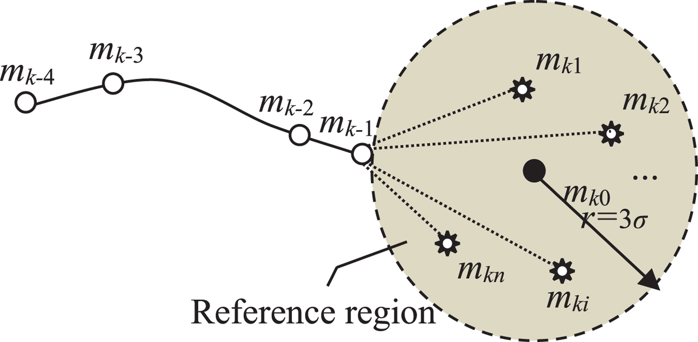
Figure 2. Basic idea of the ΔM-ICCP algorithm based on PDA.
For example, the matching length in the figure is set to 5. m k0 is the ideal magnetic value at the k-th matching point. m k1, m k2, …, m kn are the data measured n times in the presence of an interference field. m k−1, m k−2, m k−3, m k−4 are magnetic values of the other four matching points. Every two adjacent matching points of the magnetic field change satisfy Equation (3). Assuming that the interference field follows the Gaussian distribution with mean 0, variance σ 2, then according to the 3σ criteria, the magnetic measurements will fall within a circle of radius 3σ centred at m k0 with a probability of 99·74%. If the n measurements at the point are all effective, and each of them constitutes a matching sequence with m k−1, m k−2, m k−3, m k−4, then there will be n matching results when the ΔM-ICCP algorithm is executed. Considering the constraints of the kinematic performance, such as heading and velocity constraints, the position of the vehicle should be within a reasonable range. The matching result within the range is represented as a valid estimate of the vehicle position, otherwise, the matching result is invalid. By fusing all valid estimations with the PDA algorithm, the final position of the vehicle can be estimated. Then, the geomagnetic map is read to obtain the value at the calibration point, which can be used to generate the GMS in the subsequent process. Thus, the INS can be continuously corrected.
The essence of the above method is to select the positions where the vehicle is most likely to appear and to fuse them by using the PDA algorithm. Statistically speaking, if the magnetic field is measured enough, there will always be a measurement close to the ideal magnetic value, thus ensuring the fusion result of the PDA algorithm. However, the more the ΔM-ICCP algorithm is operated, the worse real-time performance it displays. Therefore, a certain number of measurements are used for fusing in practical applications, but this may lead to instability: if the measurement value deviates far from the ideal value and its matching result is considered to be effective, the fusion accuracy will be greatly reduced. Conversely, if the measurement value approximates to the ideal value, a good fusion result will be obtained. In order to avoid this problem, an improved method based on Regeneration Measurements (RMs) is proposed.
3.2.2. Improvement of the ΔM-ICCP algorithm based on RM-PDA
The basic principle of generating GMS using RMs is shown in Figure 3. The definitions of m k−1, m k−2, m k−3 and m k−4 are the same as those in Figure 2, m̂ k0 is the estimation of the ideal magnetic value at the k-th matching point, and σ̂ is the estimated standard deviation of the magnetic measurements. Three circles, centred on m̂ k0 with a radius of σ̂, 2σ̂ and 3σ̂, divide the confidence region of the magnetic measurement into three areas. The RM-PDA method respectively regenerates several possible measurements in each area and reconstitutes GMSs for geomagnetic matching and fusion. For example, in Figure 3, seven RMs are respectively generated at m̂ k0,  $\hat{m}_{k0} \pm \hat{\sigma}$,
  $\hat{m}_{k0} \pm 2\hat{\sigma}$ and
  $\hat{m}_{k0} \pm 3\hat{\sigma}$, which are denoted by
  $m'_{ki}\ (i=1, 2, \ldots, 7)$. Combining with the other four magnetic values of the matching points, several new GMSs can be formed. Then, the final position of the vehicle can be estimated by implementing the ΔM-ICCP and PDA algorithms.
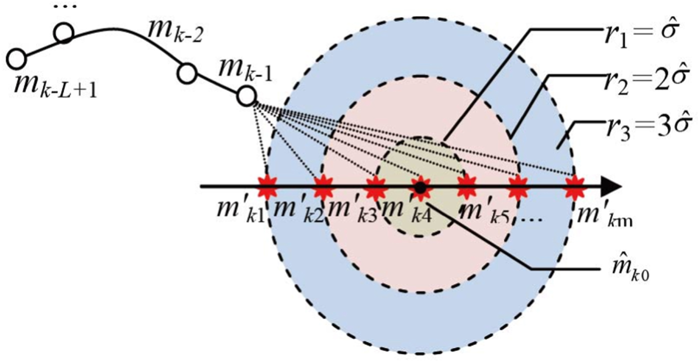
Figure 3. Schematic diagram of generating GMS based on RMs.
The improved algorithm does not directly use the measured magnetic values for matching but generates a number of controllable RMs based on the statistical characteristics of the magnetometer measurement, thereby limiting the execution time of the algorithm and greatly improving the algorithm's real-time performance. On the other hand, the RMs in r 1, r 2 and r 3 can be adjusted to avoid inaccuracy and instability when random measurements are used for matching.
3.3. Statistical characteristics evaluation of the magnetic measurements
It is difficult to measure the magnetic field of a position many times during the movement, but the vehicle will not move too far in a short time, and the magnetic variation is very slight. Compared with the influence of the interference field, the magnetic changes caused by a vehicle's movement over a very short time can be ignored. Taking the F component of the geomagnetic anomaly field model NGDC-720 (Maus, Reference Maus2010) within the scope of (71·312°, 72·312°) N, (108·5°, 109·5°) E as an example, the average magnetic variation is only about 22·5 nT/km. It is obvious that the magnetic variation is much smaller than the interference field over a short distance. Therefore, the magnetometer's measurements over a short time can be regarded as a random quantity at a position, and the parameter estimation method can be used to evaluate the statistical characteristics of the magnetic measurements.
The moment method and maximum likelihood estimation method are most commonly used in point estimation. In this paper, the first one is applied to estimate m k0 and σ2.
It is assumed that m k1, m k2, …, m kn are the values measured n times at the k-th matching point, and they follow the Gaussian distribution. Then the moment estimation of m k0 and σ2 can be expressed as:
 $$\begin{cases} \hat{m}_{k0} = \frac{1}{n} \sum_{i=1}^n m_{ki}\\ \hat{\sigma}^2 = \frac{1}{n} \sum_{i=1}^n (m_{ki} - \hat{m}_{k0})\end{cases}$$
3.4. Constraints of a vehicle's kinematic performance
If a vehicle's altitude does not change during the matching process, the GMA is executed in two-dimensional planes. Usually, the vehicle's position at the k-th matching point can be estimated by its kinematic performance at the (k-1)-th matching point.
(x k−1, y k−1) and (x k, y k) respectively denote the vehicle's positions at the k-th and (k-1)-th matching points, then according to its kinematic performance, (x k, y k) can be expressed as:
 $$\begin{cases} x_k = x_{k-1} + TV_{k-1} \cos \theta_{k-1} \\ y_k = y_{k-1} + TV_{k-1} \sin \theta_{k-1}\\ \end{cases}$$
where T is the time between the k-th and (k-1)-th matching points. V k−1 and θ k−1 are respectively the vehicle's velocity and course at the (k-1)-th matching point.
Considering the velocity and course error of a vehicle, it is assumed that its velocity is within [ $V_{k-1}^{\min}$,
  $V_{k-1}^{\max}$], and its course is within [
 $\theta_{k-1}^{\min}$,
  $\theta_{k-1}^{\max}$]. The former limits the vehicle in an annulus (denoted by U V in Figure 4(a)), which is determined by two concentric circles with radii of
  $TV_{k-1}^{\min}$ and
  $TV_{k-1}^{\max}$; the latter limits the vehicle in a sector area (denoted by U θ in Figure 4(b)). Therefore, the area of the vehicle's position U k can be represented as:
 $$U_k = U_\theta \cap U_V$$
Figure 4. Constraints of carrier's movement.
Rewriting Equation (10) in the form of analysis, the vehicle's position at the k-th matching point is:
 $$\begin{cases} (x_{k} - x_{k-1})^{2} + (y_{k} - y_{k-1})^{2} \ge (TV_{k-1}^{\min})^{2} \\ (x_{k} - x_{k-1})^2 + (y_{k} - y_{k-1})^{2} \le (TV_{k-1}^{\max})^{2} \\ \dfrac{y_{k} - y_{k-1}}{x_{k} - x_{k-1}} \ge \tan \theta_{k-1}^{\min} \\ \noalign{\vskip6pt} \dfrac{y_{k} - y_{k-1}}{x_{k} - x_{k-1}} \le \tan \theta_{k-1}^{\max} \end{cases}$$
3.5. Calculation of the associated probability
The associated probability is used to calculate the weight coefficients of all effective estimations of a vehicle's position, which is the core of the PDA algorithm. For a normal distribution with a mean of μ0 and variance of  $\sigma_{0}^{2}$, the probability that the value falls within the range of (
 $\mu_{0} - \beta \sigma_{0}$,
  $\mu_{0} + \beta \sigma_{0}$) is:
 $$P(\mu_{0} - \beta \sigma_{0} ,\mu_{0} + \beta \sigma_{0}) = erf\left(\frac{\beta }{\sqrt{2}}\right)$$
where erf(x) is the error function, which is defined as:
 $$erf(x)=\frac{\sqrt{2}}{\pi}\int_{0}^{x} e^{-\gamma^{2}}d\gamma$$
If m k1, m k2, …, m kn measured at the k-th matching point obey the normal distribution with the means of m k0 and variance of σ2, the probability that the i-th measurement at the k-th matching point comes from the ideal magnetic value can be calculated:
 $$\omega_{ki} = \int_{-\infty}^{m_{ki}} \frac{1}{\sqrt{2\pi\sigma}} \exp \left[-\frac{(x-m_{k0})^{2}}{2\sigma^{2}}\right]\hbox{d}x = 1-erf\left(\frac{m_{ki} - m_{k0}}{\sqrt{2} \sigma_0}\right),\quad i=1,2,\ldots ,n.$$
 Define a matrix  $(\boldsymbol{A})_{1\times n}$, where n is the measurement number at the k-th matching point. Once the matching result satisfies the constraints in Section 3.4, the i-th element in A is set to 1. Otherwise, the corresponding element is 0. Therefore, the associated probabilities corresponding to all effective estimations of the vehicle's positions are:
 $$[\omega_{k1}^{\prime} ,\omega _{k2}^{\prime} ,\ldots ,\omega _{kn}^{\prime}]=[\omega _{k1} ,\omega _{k2} ,\ldots ,\omega _{kn} ]^{{\rm T}} \textbf{A}$$
 Normalising  $\omega _{ki}^{\prime}$, the final associated probability of each effective estimation can be expressed as:
 $$\omega _{ki}^{\prime\prime} =\frac{\omega'_{ki}}{\sum_{i=1}^n\omega_{ki}^{\prime}},\quad i=1,2,\ldots ,n.$$
The final position of the vehicle can be estimated by:
 $$\hat{P}_k = \sum_{i=1}^n P_{ki} \omega_{ki}^{\prime \prime}.$$
where P ki is the matching result corresponding to the i-th magnetic measurement.
In practice, m k0 and σ2 can be replaced by their estimations m̂ k0 and  $\hat{\sigma }^{2}$, which was analysed in detail in Section 3.3.
4. SIMULATION EXPERIMENTS
In order to verify the proposed algorithm, a local magnetic field was randomly selected from the NGDC-720 model with latitude and longitude respectively ranging from [55·8°, 56·8°] N and [46·0°, 47·0°] E. The Kriging interpolation method (Oliver and Webster, Reference Oliver and Webster1990) was used to establish the detailed magnetic maps, as shown in Figure 5. After interpolation, the resolution of the geomagnetic map was 100 m.
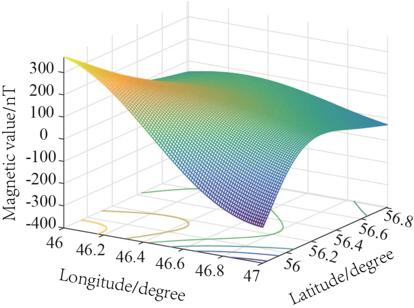
Figure 5. The geomagnetic map of a local area.
4.1. Simulation experiment of the PDA algorithm
It is assumed that the vehicle was in uniform rectilinear motion at a speed of 35 m/s in an easterly direction and its starting point was (46·069° E, 56·411° N). The initial position errors of the INS in latitude and longitude were both 300 m, and the course error was 0·5°. When the accumulated error exceeded 750 m, the fusion algorithm was used for correction.
First, the parameter of the ΔM-ICCP algorithm was determined according to Xiao et al's (2017) method. The results show that the optimal solution of the planned path was: L=6, δ=2 nT, where L refers to matching length and δ is the quantisation step of the ICCP algorithm. Then, the statistical characteristics of the magnetic measurements at the calibration point were estimated. Since the measurement results followed a normal distribution (Zhang et al., Reference Zhang, Li and Rizos2014), the simulation was performed by adding Gaussian noise to the ideal magnetic value. Assuming that the average and standard deviation of the magnetic interference were respectively 0 and 5 nT, then 100 samples were randomly selected from the simulated measurements to estimate the statistical characteristics by Equation (8).
The velocity error and course error of the vehicle were respectively set to 3 m/s and 10°. In Section 3.2.1, when the measurement number was different, the PDA fusion algorithm was implemented multiple times. The matching error is defined as the distance between the planned path and the estimated position of the vehicle. Table 1 lists the matching errors and computational time under different conditions. For each condition, three matching results are listed.
Table 1. Matching results when numbers of measurements are different.
When five measurements are used in the fusion algorithm, the matching error at the first measurement is 248·98 m, which is too large to correct the INS's accumulated error. At the second measurement, as the matching results of the ΔM-ICCP algorithm are all beyond the vehicle's restrained scope, the fusion result is invalid. Nevertheless, the matching error at the third time is 149·36 m, which is much better than the first time. When the number of measurements increases to 15, the matching result is improved to some extent, but the matching errors for three measurements are very different and the stability is poor. When the number of measurements reaches 50, the matching accuracy and stability are generally improved, but the computational time is multiplied. When the number of measurements is 70, the results are consistent with the above analysis.
In short, the PDA fusion algorithm is greatly affected by the accuracy of the magnetic measurement, and the improvement of its accuracy is at the cost of losing real-time performance.
4.2. Simulation experiment of the RM-PDA fusion algorithm
The RMs are used in the RM-PDA algorithm to overcome the shortcomings of the PDA algorithm. According to the method in Section 3.2, 13 RMs are respectively generated at m̂ k0,  $\hat{m}_{k0} \pm \frac{1}{2} \hat{\sigma}$,
  $\hat{m}_{k0} \pm \hat{\sigma}$,
  $\hat{m}_{k0} \pm \frac{3}{2} \hat{\sigma}$,
  $\hat{m}_{k0} \pm 2 \hat{\sigma}$,
  $\hat{m}_{k0} \pm \frac{5}{2} \hat{\sigma}$ and
  $\hat{m}_{k0} \pm 3 \hat{\sigma}$. The vehicle's planned path and other simulation conditions are the same as in Section 4.1.
To fully verify its performance, the RM-PDA algorithm is also compared with other five algorithms, namely the ΔM-ICCP algorithm with ideal magnetic value, the MAGCOM algorithm, the ICCP algorithm with magnetic interference, the ΔM-ICCP algorithm with interference and the PDA fusion algorithm with interference. The number of measurements of the PDA algorithm is the same as for the RM-PDA algorithm. Considering the compensation effect (Liu et al., Reference Liu, Zhang, Pan and Shan2016), the standard deviations of the magnetic interference are set as 1 nT, 3 nT, 5 nT, 7 nT and 9 nT.
All algorithms are executed multiple times, Figure 6 shows their matching errors (in logs) at each time, and Table 2 lists the average matching errors of 13 repetitions.

Figure 6. Comparisons of different algorithms under different interferences.
Table 2. Average matching errors of different algorithms.

When there is no interference, the matching error of the ΔM-ICCP algorithm is 11·65 m, in a very stable state. While different interferences exert a large influence on the ICCP, MAGCOM and ΔM-ICCP algorithms, their matching results indicate large uncertainty in interference fields. In Figure 6, some of their matching errors are even larger than the accumulated error of the INS. This means that the matching algorithm has diverged and is unavailable to correct the INS. When the standard deviation of magnetic interference is 1 nT, most of the results of MAGCOM algorithm are effective, but when the standard deviation is larger than 3 nT, its performance is significantly reduced. In addition, when the interference standard deviation is 8 nT and 9 nT, the MAGCOM, ICCP and ΔM-ICCP algorithms show little difference. This illustrates that these algorithms are unavailable if the interference is too strong.
In contrast, the accuracy of the PDA algorithm has been improved to some extent, and the matching results are convergent under different conditions, but its anti-interference performance and accuracy still need to be enhanced. The RM-PDA algorithm, however, has the highest accuracy under different interferences and shows better anti-interference performance and stability. Therefore, the RM-PDA algorithm is available to modify the INS's accumulated error.
4.3. Matching probabilities of different algorithms
Matching Probability (MP) (Huynh et al., Reference Huynh, Do and Yoo2017) measures the reliability of the matching results. Once the geomagnetic matching area and interference field are confirmed, the MP can be used to evaluate the algorithm's performance. However, its definition is not currently unified. In this paper, according to Inglada and Giros's (Reference Inglada and Giros2004) method, MP is defined as the correct registration rate, namely:
 $$P_{{\rm MA}} =\frac{\sum_{p\in {\rm MA}} {N(p)}}{N_{{\rm MA}}}$$
where MA is a selected matching area, and N MA represents the total number of matchings in MA.  $\sum_{p\in {\rm MA}} {N(p)} $ counts the successful matches, and p is a reference point. In the matching process, each grid point in the MA is used as a reference point to participate in the matching algorithm.
A number of areas with a size of  $2\,{\rm km}\times 2\,{\rm km}$ were randomly selected from the NGDC-720 model, and the MPs of different algorithms were calculated under different conditions. Suppose that the matching length is 5, and the quantisation step of the ΔM-ICCP algorithm is 1 nT. The other parameters are the same as in Section 4.1. When the matching error is less than 200 m, the matching is considered to be successful. Figure 7 shows the MPs of the area whose longitude range is
  $56{\cdot}082^{\circ}\sim 56{\cdot}101^{\circ}\, {\rm N}$, latitude range is
  $46{\cdot}320^{\circ}\sim 46{\cdot}339^{\circ}\,{\rm E}$.

Figure 7. Matching probabilities of different algorithms.
The results show that when the standard deviation of the interference is under 0·5 nT, both the ICCP algorithm and ΔM-ICCP algorithm are reliable, and their MPs are close to 1. When the interference increases, the MPs decline significantly at first, and then gradually tail to 0. On the other hand, the MPs of ΔM-ICCP algorithm are slightly higher than the ICCP algorithm under different conditions, which is mainly because the former uses more magnetic information when their matching lengths are the same. In contrast, when the interference standard deviation is between 0·1 nT and 3 nT, the MPs of RM-PDA algorithm are all equal to 1, which means that even if the interference field affects the matching algorithm, all the matching errors are within the pre-set threshold. Although the MP of the RM-PDA algorithm reduces with increasing interference, its performance is still better than the other two algorithms. In short, the RM-PDA algorithm has better performance as a whole under different interferences.
4.4. Algorithm comparison on another path
In order to further analyse the performance of the proposed algorithm, 50 geomagnetic areas were randomly selected according to different magnetic environments. Taking one of these areas as an example, the following shows the matching process.
The simulation parameters were set as follows: the vehicle was in uniform rectilinear motion at a speed of 35 m/s from point (46·439° E, 56·361° N), the angle between its moving direction and east was 30°. The initial position errors of the INS in latitude and longitude were both 300 m, and the course error was 1°. When its accumulated error exceeded 500 m, the fusion algorithm was used to correct it.
According to Xiao et al.’s (2017) method, at the calibration point of this path, the optimal matching length (L) and quantisation step (δ ) were: L=5, δ=3 nT. Then the statistical characteristics of the magnetic measurements at the calibration point were estimated and the PDA algorithm and RM-PDA algorithm were executed. In the RM-PDA algorithm, the velocity error and course error were respectively set to 3 m/s and 10°.
Table 3 lists the average matching errors for 12 times matching. As shown, when there is no interference, the matching error of the ΔM-ICCP algorithm was 13·06 m. Although the ΔM-ICCP algorithm shows smaller matching errors, the performances of the ICCP and ΔM-ICCP algorithms reduced significantly with the increase of interference. When the standard deviation of interference was larger than 3 nT, the matching error of ICCP was 775·39 m, which exceeded the accumulated error of INS. This also shows that most results of the MAGCOM algorithm were ineffective. In contrast, the matching results of the PDA and RM-PDA algorithms were all effective. Meanwhile, all the errors of the RM-PDA algorithm were in one magnetic grid (100 m), and the results were more stable.
Table 3. Algorithm comparison results on another path.

The above analysis is consistent with the results in Section 4.2. Simulation experiments prove that the conclusions still hold in other geomagnetic areas. As a result, the effectiveness of the proposed algorithm is verified.
5. SEMI-PHYSICAL EXPERIMENTS
In order to test the proposed algorithm in a relatively real environment, a semi-physical verification system was constructed. As shown in Figure 8, the system mainly consists of five parts: a three-axis Helmholtz coil, a high-precision current source, a magnetometer, a magnetic simulation computer and a navigation computer. Their functions and parameters were as follows:

Figure 8. The semi-physical system.
The three-axis Helmholtz coil was used to simulate the geomagnetic environment. The Helmholtz coil used in this study can generate a magnetic field from −20,000 nT to 20,000 nT.
The high-precision current source was used to generate current and control the magnetic field in the Helmholtz coil. The system used a KEITHLEY 6220 current source that can produce a DC current from 100 fA to 100 mA.
The magnetometer was placed in the Helmholtz coil to measure the magnetic field inside the coil. The resolution of the magnetometer was 1 nT.
The magnetic simulation computer was used to calculate the magnetic values on the planned path based on the geomagnetic model, and the corresponding current was calculated according to the relationship between the magnetic field and the current in the Helmholtz coil.
The navigation computer was used to plan the vehicle's path, record the magnetometer's outputs, implement the GMA and correct the INS's accumulated error.
The semi-physical verification system was placed in the laboratory, and the surrounding electromagnetic devices and the magnetometer affected the magnetic measurements. It was assumed that other kinds of interference fields follow a normal distribution, which were added to the Helmholtz coil through the current source.
The vehicle was assumed to move along the path in Section 4.1, its course error was 0·5° and the initial position errors of the INS in longitude and latitude are both 300 m. Other simulation parameters were the same as in Section 4.1. As the planned path and calibration point do not change, L=6 and δ=2 nT are still the optimal parameters of the ΔM-ICCP algorithm.
Different interferences were added to the Helmholtz coil and the magnetometer's outputs were recorded. Since the distribution of the real measurements was unknown, moment estimation and the Kolmogorov-Smirnov (K-S) test (Al-Labadi and Zarepour, Reference Al-Labadi and Zarepour2017) were used to evaluate and verify the statistical characteristics. Figure 9 compares the Cumulative Distribution Function (CDF) of the normalised measurements in one experiment with the standard normal distribution. It was proved that the magnetometer's measurements still obey the normal distribution in the laboratory environment and under the interference of normal distribution. It also shows that the estimated statistical characteristics are valid.

Figure 9. K-S test of magnetometer measurements.
Based on the estimated characteristics, the PDA and RM-PDA algorithms were respectively conducted. The RMs of the RM-PDA algorithm remained unchanged. The measurements of the PDA algorithm were randomly selected, and the number of them were the same as the RM-PDA algorithm. Figure 10 and Table 4 record the matching results in different conditions.

Figure 10. Matching results of semi-physical system in different conditions.
Table 4. Matching errors in different conditions.

Many other simulation and semi-physical experiments have been carried out and the above conclusions were valid with regard to these results as well.
6. CONCLUSIONS
In order to enhance the accuracy and anti-interference performance of the ICCP algorithm, the delta modulation and PDA algorithm were applied. The feasibility and effectiveness of the algorithm were verified by simulation and semi-physical experiments. The main contributions of this paper are as follows:
(1) The ΔM-ICCP algorithm can assess the GMS to participate in the matching process and find the optimal matching length, which guarantees the accuracy and real-time performance of the proposed algorithm.
(2) Based on the estimated statistical characteristics of the magnetic measurements, the RM-PDA algorithm regenerates a certain number of measurements for matching, which enhances the anti-interference performance and stability of the algorithm.
The interference field that satisfies the Gaussian distribution is added to the geomagnetic model, and the instrument error and the interferences in the laboratory are considered in this paper. However, in practice, the magnetic environment is more complicated. In future studies, the proposed algorithm will be fully evaluated in a real environment.


