


1. Introduction
In contrast to rigid-link robotic arms, continuum arms are flexible structures with the ability of continuous bending along the backbone. These arms are inspired from intrinsic capabilities of natural organisms like snakes, octopus arms, elephant trunks, and mammalian tongues. The unique features of these arms like manipulating in unstructured environments, grasping unknown objects, safe operation as well as dexterity make them a popular research area [Reference Saab, Rone and Ben-Tzvi1].
Obtaining dynamics (forward dynamics (FD) and inverse dynamics (ID)) and kinematics (forward kinematics (FK) and inverse kinematics (IK)) in continuum manipulators encounter several challenges. These challenges are originated from high nonlinearities, uncertainties, friction, shear, and so on, which limit modeling accuracy and increase computation time. Modeling can be considered as the first and most fundamental step regarding its influence in further applications, including path planning [Reference Li and Xiao2], optimization [Reference Xu, Zhao and Zheng3], grasping [Reference Braganza, Dawson, Walker and Nath4], and control [Reference Cobos-Guzman, Palmer and Axinte5]. Despite the extensive published papers in the field of kinematics modeling, only a few investigations have been dedicated to dynamics modeling of these manipulators considering high complexity, particularly in spatial motions. Most of the conducted researches were based on the development of corresponding kinematics models, through which higher errors would be generated [Reference Thuruthel, Falotico, Renda and Laschi6]. Generally, prior investigations in modeling field can be categorized into three groups of analytical, numerical, and data-driven approaches, which would be explained in the following sections.
1.1. Analytical methods
These methods are referred to the methods, through which analytical solution can be obtained from closed-form equations by assuming some simplifying assumptions. Among the most commonly used simplifications, it can be mentioned to planar motion, constant curvature (CC), and neglection of nonlinear terms assumptions. Bamdad et al. [Reference Bamdad and Bahri7] introduced an analytical procedure using modified Denavit–Hartenberg (D–H) technique for obtaining FK of continuum manipulators with piecewise CC assumption and used it for real-time control of manipulator. In another study by Neppalli [Reference Neppalli, Csencsits, Jones and Walker8], a closed-form analytical solution was developed for a multi-section continuum manipulator by discretizing the manipulator into several single-section manipulators. However, error propagation for multi-section case was not addressed. Falkenhahn et al. [Reference Falkenhahn, Mahl, Hildebrandt, Neumann and Sawodny9] used a lumped-mass and CC assumptions along with the analytical derivatives in order to establish a balance between forces and energies. Both FD and ID models were obtained; however, only planar case with neglecting torsional effects was studied. Generally, key advantage of analytical approaches is the provision of closed-form solution, which can be implemented easily in further applications, especially for control purposes. Nevertheless, problems resulted from simplifying assumptions, including poor performance, deviation from experimental results, and incapability in providing exact model can be considered as disadvantages.
1.2. Numerical methods
To solve the mentioned deficiencies and difficulties, numerical approaches have been suggested by many researchers. In a research by Chikhaoui et al. [Reference Chikhaoui, Lilge, Kleinschmidt and Burgner-Kahrs10], FK of a tendon-driven continuum manipulator with extensible segments was determined numerically using two procedures of Cosserat rod theory and beam theory. Despite the higher accuracy of former procedure, latter one provided lower computational cost. Peyron et al. [Reference Peyron, Boehler, Rabenorosoa, Nelson, Renaud and Andreff11] obtained the kinematics model of a continuum manipulator by solving boundary value problem. In this study, the manipulator was discretized along its backbone and obtained nonlinear equations for each section were solved numerically. Besides, experimental tests were executed on a magnetic continuum manipulator for the sake of validation. However, no comparison was performed to evaluate the effectiveness of the proposed approach with other numerical approaches. In a study by Kang et al. [Reference Kang, Branson, Zheng, Guglielmino and Caldwell12], a pneumatically driven continuum manipulator was discretized to a number of serially connected parallel mechanisms and the kinematics/dynamics were derived with the help of rigid body dynamics. Habibi et al. [Reference Habibi, Yang, Godage, Kang, Walker and Branson13] introduced a lumped-mass model for flexible surfaces subjected to large deflection as a result of actuating with two continuum manipulators. The equations of motion for discretized masses were derived through general Newtonian principle. In another study, Kim et al. [Reference Kim, Cheng, Diakite, Gullapalli, Simard and Desai14] obtained the FK of three-section tendon-driven continuum manipulator through circular arcs assumption. The derived equations from twist method were solved numerically and validated through experimental tests. In refs. [Reference Dehghani and Moosavian15,Reference Dehghani and Moosavian16], Dehgani et al. presented a dynamic modeling approach for continuum manipulator, which used Cosserat rod theory with some realistic simplifying assumptions to reduce computational cost. In addition, a method for canceling the error of numerical integrations was introduced to enhance the computations speed. In general, main advantage of numerical approach is the provision of more exact model in which some nonlinearities and uncertainties can be considered. However, despite the improvement in accuracy, system complexity and computational cost would be increased. Hence, suitability of these approaches for online purposes would be weakened. Moreover, convergence is not guaranteed in most of the numerical approaches, so the solutions are probable to be trapped in the local solution.
1.3. Data-driven methods
Regarding the aforementioned challenges in previous approaches, recently, data-driven modeling (DDM) has been proposed. This type of modeling can be defined as establishing a relation between inputs and outputs of system without using explicit mathematical equations [Reference Solomatine, See and Abrahart17]. In a study by Li et al. [Reference Li, Kang, Branson and Dai18], a DDM procedure was applied to determine a mapping from actuator to position signals of a pneumatically driven continuum manipulator. The estimation of online Jacobian was accomplished using adaptive Kalman filter with the ability of capturing instantaneous changes in Jacobian. In another research by Tan et al. [Reference Tan, Gu and Ren19], parameters of kinematics model were identified experimentally to cover existing uncertainties in parameters and joint inputs. However, the proposed scheme was validated only for in-plane motions. Recently, Jackes et al. [Reference Jakes, Ge and Wu20] proposed a recurrent neural network-based approach. This approach avoided the complexity of mathematical modeling, while capturing the mechanical and electrical nonlinear effects of the system. The proposed model related the actuation signals to the force measurement; however, it was validated only for a single-segment three-tendon continuum manipulator. In a study by Thuruthel et al. [Reference Thuruthel, Falotico, Renda and Laschi6], a methodology was suggested for learning the FD of soft manipulator with the use of model-free neural network-based approach for the first time. They declared that their method provides easier implementation and improved accuracy compared to other dynamics models. It should be noted that learning inverse model in redundant manipulators often encounters some problem regarding the nonuniqueness of solutions. Several approaches have been proposed for overcoming this problem, such as distal supervised learning [Reference Melingui, Merzouki, Mbede, Escande, Daachi and Benoudjit21], learning in velocity level [Reference D’Souza, Vijayakumar and Schaal22], path-based sampling approach (goal babbling) [Reference Rolf and Steil23], and multiple local learning procedure [Reference Vannucci, Falotico, Di Lecce, Dario and Laschi24]. Basically, the main benefit of DDM is capturing the whole system behavior which was partially discarded in previous approaches. In addition, adaptability to a wide range of manipulators, or in other words, robot-independent structure is the other potential advantage. However, requirement for higher datasets to attain an appropriate model may affect the computational time.
Inclusion of contact forces in modeling is an important issue that should be considered. Involved forces can be classified to small-valued and large-valued forces in terms of their magnitude regarding the stiffness of manipulator, inertia, velocity, duration, and location of contact [Reference Thuruthel, Shih, Laschi and Tolley25]. In former group, small undesired contact forces can be covered with small approximation error by neural networks [Reference Grassmann, Modes and Burgner-Kahrs26]. However, addition of second-class forces imposes higher complexity in analytical and numerical procedures; in this regard, some data-driven methods were presented [Reference Jakes, Ge and Wu20, Reference Thuruthel, Shih, Laschi and Tolley25]. Thuruthel et al. [Reference Thuruthel, Shih, Laschi and Tolley25] suggested a data-driven technique using force data obtained from single load cell embedded on the end effector of manipulator. With the help of gathered data, they established a neural network-based learning model for predicting the force.
By reviewing the available literature, lack of a general framework for obtaining kinematics and dynamics with applicability for different types/scales of continuum manipulators and capability of dealing with uncertainties, nonlinearities, and load carrying is sensed. Moreover, in most of the conducted researches, ID problem was mostly discarded considering its higher complexity. To overcome these deficiencies, in this paper, a DDM approach is proposed to consider the dynamic motion of manipulator using nonlinear autoregressive network with exogenous inputs (NARX) model.
The main contributions of the present paper can be summarized as follows:
-
• Proposing a general framework with maximal applicability for dynamics modeling (FD/ID) of continuum manipulators, which can be also used for kinematics modeling (FK/IK).
-
• Eliminating the need for solving complex equations by the use of data-driven approach.
-
• Capturing existing nonlinearities and uncertainties in parameters and the structure of continuum manipulator.
-
• Providing a simple and real-time solution with high consistency to real experimental setup in spatial motions for further applications, especially control schemes.
-
• Proposing a straightforward algorithm for path tracking of continuum manipulator in the presence and absence of obstacles as well as load carrying maneuver.
-
• Investigating the scalability of proposed procedure for manipulators with different numbers of sections.
-
• Implementation of proposed procedure on experimental setup of RoboArm and simulation setup based on Cosserat rod theory.
The rest of the paper is organized as follows: in Section 2, the problem is defined and the proposed procedure for kinematics/dynamics modeling of continuum manipulator in three-dimensional space is described. In the following section, the inverse problem is explored; additionally, path tracking and load carrying features are evaluated. Section 4 is dedicated to the description of studied systems: simulation setup based on Cosserat rod theory and the experimental setup of RoboArm. The results of implementing the proposed procedure on both simulation and experimental setups are provided and discussed in Section 5. Finally, main findings of this investigation are provided in the conclusion section.

Figure 1. Schematic of a two-section continuum manipulator consisting of a backbone, six servomotors, six tendons, and several spacers. The motor position [P] and tendon tension [T] are the system inputs and the position of end effector [X] is the system output.
2. Problem Definition
The considered system in this study is a continuum manipulator representing a multi-input multi-output (MIMO) system with n sections, r inputs, and m outputs. The schematic of a two-section continuum manipulator is illustrated in Fig. 1. According to this figure, the system is consisted of a backbone, tendons for actuating manipulator, and spacers for keeping tendons parallel with respect to the backbone. The manipulator is a two-section system (n=2) and six servomotors (r=6) are used for positioning the end effector (m=3). The inputs are motor position/tendon tension
 ${\left[ {{\textbf{P/T}}} \right]_{{\textbf{j}} = 1,2, \ldots ,n}}$
of jth section (
${\left[ {{\textbf{P/T}}} \right]_{{\textbf{j}} = 1,2, \ldots ,n}}$
of jth section (
 $j \in \left\{ {1, \ldots ,n} \right\}$
), and the outputs are position/orientation of end effector,
$j \in \left\{ {1, \ldots ,n} \right\}$
), and the outputs are position/orientation of end effector,
 $\left[ {\textbf{X}} \right]$
. The goal is to develop the best model (
$\left[ {\textbf{X}} \right]$
. The goal is to develop the best model (
 ${{\textbf{M}}^*}$
) for a continuum manipulator among the candidate models as follows:
${{\textbf{M}}^*}$
) for a continuum manipulator among the candidate models as follows:
 \begin{align}{{\textbf{M}}^*} = \left\{ {{\textbf{M}}\left( \theta \right)|\theta \in {D_m}} \right\}\end{align}
where
 ${\textbf{M}}(\theta )$
is the model structure, which can be ARX, NARX, and ARMAX, etc., and should be selected on the basis of an appropriate criterion. In addition,
${\textbf{M}}(\theta )$
is the model structure, which can be ARX, NARX, and ARMAX, etc., and should be selected on the basis of an appropriate criterion. In addition,
 ${D_m}$
is an index set of interest. To this aim, a data-driven system identification (SI) procedure is proposed.
${D_m}$
is an index set of interest. To this aim, a data-driven system identification (SI) procedure is proposed.
2.1. Data-driven identification procedure for modeling
The proposed procedure for modeling continuum manipulator is depicted in Fig. 2. According to this flowchart, proposed SI contains four main steps. These steps are known as the determination of model inputs/excitation signals, selecting model structure/parameters, identification procedure, and evaluation steps, which are detailed in the following subsection (for more details, refer to refs. [Reference Parvaresh, Moosavi and Moosavian27–Reference Parvaresh and Moosavian29]).
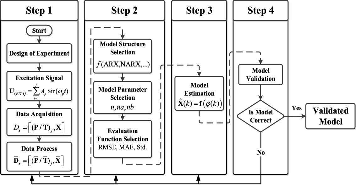
Figure 2. The main steps for modeling continuum manipulator through data-driven system identification procedure for obtaining a validated model.
2.1.1. Inputs and excitation signals
Identification procedure is conducted based on processed input–output data,
 ${\overline{\textbf{D}}}_{s} = [(\overline{\textbf{P}}/\overline{\textbf{T}})_{J},\overline{\textbf{X}}]$
, from continuum manipulator. If reasonable and appropriate distribution is assumed for data, high-precision model would be obtained with higher amount of training data. The overall real operating workspace of manipulator should be covered during data acquisition process. In addition, sampling time should be considered small enough to capture small changes in model output so that
${\overline{\textbf{D}}}_{s} = [(\overline{\textbf{P}}/\overline{\textbf{T}})_{J},\overline{\textbf{X}}]$
, from continuum manipulator. If reasonable and appropriate distribution is assumed for data, high-precision model would be obtained with higher amount of training data. The overall real operating workspace of manipulator should be covered during data acquisition process. In addition, sampling time should be considered small enough to capture small changes in model output so that
 \begin{align} {\rm{for }}\;{x_m} \in {\textbf{X}}:\;\;{\rm{ }}{x_m}(k - i) \simeq {x_m}(k - i - 1) \end{align}
where
 ${\rm{ }}{x_m}(k - i)$
and
${\rm{ }}{x_m}(k - i)$
and
 ${x_m}(k - i - 1)$
are two subsequent outputs and k is the time sample. For n-section manipulator with three tendons in each section, we have
${x_m}(k - i - 1)$
are two subsequent outputs and k is the time sample. For n-section manipulator with three tendons in each section, we have
 $${{{\left[ {{\bf{P}}/{\bf{T}}} \right]}_{j = 1,2, \ldots ,n}} = \left[ {\matrix{
{{{\left( {{\bf{P}}/{\bf{T}}} \right)}_{\bf{1}}}} \cr
\vdots \cr
{{{\left( {{\bf{P}}/{\bf{T}}} \right)}_{\bf{j}}}} \cr
} } \right] = \left[ {\matrix{
{{{\left( {P/T} \right)}_{1,1}}} & {{{\left( {P/T} \right)}_{1,3}}} & {{{\left( {P/T} \right)}_{1,5}}} \cr
\vdots & \vdots & \vdots \cr
{{{\left( {P/T} \right)}_{j,j}}} & {{{\left( {P/T} \right)}_{j,j + 2}}} & {{{\left( {P/T} \right)}_{j,j + 4}}} \cr
} } \right]}$$
$${{{\left[ {{\bf{P}}/{\bf{T}}} \right]}_{j = 1,2, \ldots ,n}} = \left[ {\matrix{
{{{\left( {{\bf{P}}/{\bf{T}}} \right)}_{\bf{1}}}} \cr
\vdots \cr
{{{\left( {{\bf{P}}/{\bf{T}}} \right)}_{\bf{j}}}} \cr
} } \right] = \left[ {\matrix{
{{{\left( {P/T} \right)}_{1,1}}} & {{{\left( {P/T} \right)}_{1,3}}} & {{{\left( {P/T} \right)}_{1,5}}} \cr
\vdots & \vdots & \vdots \cr
{{{\left( {P/T} \right)}_{j,j}}} & {{{\left( {P/T} \right)}_{j,j + 2}}} & {{{\left( {P/T} \right)}_{j,j + 4}}} \cr
} } \right]}$$
For simplicity, from now on, inputs are shown by
 $\left[ {\textbf{T}} \right]$
instead of
$\left[ {\textbf{T}} \right]$
instead of
 $\left[ {{\textbf{P/T}}} \right]$
. In studied manipulator, which is a two-section, six-tendon manipulator, input vector is defined as:
$\left[ {{\textbf{P/T}}} \right]$
. In studied manipulator, which is a two-section, six-tendon manipulator, input vector is defined as:
 $$\matrix{
{{{\left[ {\bf{T}} \right]}_{j = 1,2}} = \left[ {\matrix{
{{{\bf{T}}_{\bf{1}}}} \cr
{{{\bf{T}}_2}} \cr
} } \right] = \left[ {\matrix{
{{T_{1,1}}\quad {T_{1,3}}\quad {T_{1,5}}} \cr
{{T_{2,2}}\quad {T_{2,4}}\quad {T_{2,6}}} \cr
} } \right]} \hfill \cr
} $$
$$\matrix{
{{{\left[ {\bf{T}} \right]}_{j = 1,2}} = \left[ {\matrix{
{{{\bf{T}}_{\bf{1}}}} \cr
{{{\bf{T}}_2}} \cr
} } \right] = \left[ {\matrix{
{{T_{1,1}}\quad {T_{1,3}}\quad {T_{1,5}}} \cr
{{T_{2,2}}\quad {T_{2,4}}\quad {T_{2,6}}} \cr
} } \right]} \hfill \cr
} $$
Additionally, outputs vector is
 $$\matrix{
{{\bf{X}} = \left[ {\matrix{
{{x_{ee}}\quad {y_{ee}}\quad {z_{ee}}} \cr
} } \right]} \hfill \cr
} $$
$$\matrix{
{{\bf{X}} = \left[ {\matrix{
{{x_{ee}}\quad {y_{ee}}\quad {z_{ee}}} \cr
} } \right]} \hfill \cr
} $$
In the above equation,
 ${x_{ee}},{\rm{ }}{y_{ee}}$
and
${x_{ee}},{\rm{ }}{y_{ee}}$
and
 ${z_{ee}}$
are the positions of end effector along X-, Y-, and Z-axis with respect to the manipulator base,
${z_{ee}}$
are the positions of end effector along X-, Y-, and Z-axis with respect to the manipulator base,
 ${\rm{O = }}\left\{ {{{\rm{x}}_{\rm{0}}}{\rm{, }}\,{{\rm{y}}_{\rm{0}}}{\rm{, }}\,{{\rm{z}}_{\rm{0}}}} \right\}$
. Therefore, collected datasets for
${\rm{O = }}\left\{ {{{\rm{x}}_{\rm{0}}}{\rm{, }}\,{{\rm{y}}_{\rm{0}}}{\rm{, }}\,{{\rm{z}}_{\rm{0}}}} \right\}$
. Therefore, collected datasets for
 ${n_{data}}$
independent points are defined as
${n_{data}}$
independent points are defined as
 $${\left[ {\matrix{
{{{\left( {\bf{T}} \right)}_{j = 1,2}}\quad {\bf{X}}} \cr
} } \right]_{l = 1,2, \ldots ,{n_{data}}}}$$
. Different excitation signals can be used for identifying unknown systems. According to ref. [Reference Nelles30], model identified with sine excitation has an excellent quality in the excited frequencies. So, a combination of sine signals would be an appropriate selection for our continuum manipulator as shown in Equation (6):
$${\left[ {\matrix{
{{{\left( {\bf{T}} \right)}_{j = 1,2}}\quad {\bf{X}}} \cr
} } \right]_{l = 1,2, \ldots ,{n_{data}}}}$$
. Different excitation signals can be used for identifying unknown systems. According to ref. [Reference Nelles30], model identified with sine excitation has an excellent quality in the excited frequencies. So, a combination of sine signals would be an appropriate selection for our continuum manipulator as shown in Equation (6):
 \begin{align}{{\textbf{U}}_{{{\left( {\textbf{T}} \right)}_j}}} = {A_1}\;{\mathop{\rm Sin}\nolimits} ({\omega _1}t) + {A_2}\;{\mathop{\rm Sin}\nolimits} ({\omega _2}t) + \ldots \,\,\,\, = \sum\limits_{i = 1}^p {{A_p}\;{\mathop{\rm Sin}\nolimits} ({\omega _p}t)} \end{align}
where
 $p$
is the number of sine signals,
$p$
is the number of sine signals,
 ${A_p}$
and
${A_p}$
and
 ${\omega _p}$
are the corresponding amplitude and frequency of pth signal, respectively. The workspace of excited manipulator besides data gathering procedure is shown in Fig. 3.
${\omega _p}$
are the corresponding amplitude and frequency of pth signal, respectively. The workspace of excited manipulator besides data gathering procedure is shown in Fig. 3.

Figure 3. (a) Data gathering procedure of required dataset for learning and (b) three-dimensional workspace of the continuum manipulator resulted from excitation signals.
2.1.2. Model structure
Choosing an appropriate structure for model has an important role in determining the number of required parameters, convergence, and computational cost. The model can be described by a mapping
 ${\textbf{M}}({\mathbb{R}^r} \mapsto {\mathbb{R}^m})$
from inputs space (
${\textbf{M}}({\mathbb{R}^r} \mapsto {\mathbb{R}^m})$
from inputs space (
 $\mathbb{R}$
r
) to outputs space (
$\mathbb{R}$
r
) to outputs space (
 $\mathbb{R}$
m
) as:
$\mathbb{R}$
m
) as:
 \begin{align}{\left[ {{\textbf{X}}(k + 1)} \right]_{m \times 1}} = {\textbf{M}}{\left( \begin{array}{l}{\textbf{T}}(k), \ldots ,{\textbf{T}}(k - na),\\[5pt]
{\rm{ }}{\textbf{X}}(k), \ldots {\textbf{X}}(k - nb)\end{array} \right)_{(m + r) \times 1}}\end{align}
\begin{align}{\left[ {{\textbf{X}}(k + 1)} \right]_{m \times 1}} = {\textbf{M}}{\left( \begin{array}{l}{\textbf{T}}(k), \ldots ,{\textbf{T}}(k - na),\\[5pt]
{\rm{ }}{\textbf{X}}(k), \ldots {\textbf{X}}(k - nb)\end{array} \right)_{(m + r) \times 1}}\end{align}
In the above equation,
 $$\left[ {\matrix{
{{\bf{X}}(k)\quad \ldots \quad {\bf{X}}(k - nb)} \cr
} } \right]$$
are current/previous outputs and
$$\left[ {\matrix{
{{\bf{X}}(k)\quad \ldots \quad {\bf{X}}(k - nb)} \cr
} } \right]$$
are current/previous outputs and
 $$\left[ {\matrix{
{{\bf{T}}(k)\quad \ldots \quad {\bf{T}}(k - na)} \cr
} } \right]$$
represent current/previous inputs. In addition,
$$\left[ {\matrix{
{{\bf{T}}(k)\quad \ldots \quad {\bf{T}}(k - na)} \cr
} } \right]$$
represent current/previous inputs. In addition,
 $na$
and
$na$
and
 $nb$
are the respective numbers of previous inputs and outputs. Among different structures that can be used for M, recurrent dynamic network of NARX model, which is a nonlinear expansion of ARX model, is selected considering the nonlinear and dynamic nature of the system. The ARX representation for single-input single-output (SISO) system is defined as:
$nb$
are the respective numbers of previous inputs and outputs. Among different structures that can be used for M, recurrent dynamic network of NARX model, which is a nonlinear expansion of ARX model, is selected considering the nonlinear and dynamic nature of the system. The ARX representation for single-input single-output (SISO) system is defined as:
 \begin{align}\hat X(k) = {b_1}T(k - 1) + \ldots . + {b_l}T(k - na)\, - {a_1}X(k - 1) - \ldots - {a_l}X(k - nb)\end{align}
where
 $\hat X(k)$
is the estimation of model output in current time regarding previous information of
$\hat X(k)$
is the estimation of model output in current time regarding previous information of
 $T(k - na) \in \mathbb{R}$
and
$T(k - na) \in \mathbb{R}$
and
 $x(k - nb) \in \mathbb{R}$
. Also,
$x(k - nb) \in \mathbb{R}$
. Also,
 ${a_l}$
and
${a_l}$
and
 ${b_l}$
are respective constant coefficients for outputs and inputs that should be specified through identification. By substituting the known linear function by a nonlinear unknown function of
${b_l}$
are respective constant coefficients for outputs and inputs that should be specified through identification. By substituting the known linear function by a nonlinear unknown function of
 $f(.)$
, NARX representation can be obtained as follows:
$f(.)$
, NARX representation can be obtained as follows:
 \begin{align} \hat X(k) = f\left( {\varphi (k)} \right) \end{align}
where
 $\varphi (k)$
is the regression vector and defined as:
$\varphi (k)$
is the regression vector and defined as:
 \begin{align}\varphi (k) = {\left[ {T(k - 1) \ldots T(k - na){\rm{ }}\;X(k - 1) \ldots X(k - nb)} \right]^T}\end{align}
So, Equation (9) can be rewritten as:
 \begin{align}\hat X(k) = f\left( {T(k - 1), \ldots ,T(k - na),\;X(k - 1), \ldots ,X(k - nb)} \right)\end{align}
By extending this formula to r-input m-output MIMO system, we have
 \begin{align}\left[ \hat{\textbf{X}}(k) \right] = {\textbf{f}}\left( \begin{array}{l}{T_1}(k - 1), \ldots ,{T_1}(k - na), \ldots ,{T_r}(k - 1), \ldots ,{T_r}(k - na),\\[5pt]
{X_1}(k - 1), \ldots .{X_1}(k - nb), \ldots ,{X_m}(k - 1), \ldots ,{X_m}(k - nb)\end{array} \right)\end{align}
\begin{align}\left[ \hat{\textbf{X}}(k) \right] = {\textbf{f}}\left( \begin{array}{l}{T_1}(k - 1), \ldots ,{T_1}(k - na), \ldots ,{T_r}(k - 1), \ldots ,{T_r}(k - na),\\[5pt]
{X_1}(k - 1), \ldots .{X_1}(k - nb), \ldots ,{X_m}(k - 1), \ldots ,{X_m}(k - nb)\end{array} \right)\end{align}
where
 ${\rm{f}}(.) \in {\mathbb{R}^{m \times r}}$
is a matrix of
${\rm{f}}(.) \in {\mathbb{R}^{m \times r}}$
is a matrix of
 $m \times r$
nonlinear functions from
$m \times r$
nonlinear functions from
 ${\mathbb{R}^r} \to {\mathbb{R}^m}$
. Equation (12), which is written in scalar form, can be represented in a vector form for discrete-time nonlinear MIMO system as:
${\mathbb{R}^r} \to {\mathbb{R}^m}$
. Equation (12), which is written in scalar form, can be represented in a vector form for discrete-time nonlinear MIMO system as:
 \begin{align}\left[ \hat{\textbf{X}}(k) \right] = {\textbf{f}}\left( {{\textbf{T}}(k - 1), \ldots ,{\textbf{T}}(k - na),{\textbf{X}}(k - 1), \ldots .{\textbf{X}}(k - nb)} \right)\end{align}
where
 ${\textbf{X}}$
and
${\textbf{X}}$
and
 ${\textbf{T}}$
are
${\textbf{T}}$
are
 $m \times 1$
and
$m \times 1$
and
 $r \times 1$
vectors and defined as:
$r \times 1$
vectors and defined as:
 \begin{align}\begin{array}{l}{\textbf{X}}(k) = {\left[ {\begin{array}{*{20}{c}}{{x_1}(k)}\;\;\;{ \ldots }\;\;\;{{x_m}(k)}\end{array}} \right]_{m \times 1}}^T\\[7pt]
{\textbf{T}}(k) = {\left[ {\begin{array}{*{20}{c}}{{T_1}(k)}\;\;\;{ \ldots }\;\;\;{{T_r}(k)}\end{array}} \right]_{r \times 1}}^T\end{array}\end{align}
\begin{align}\begin{array}{l}{\textbf{X}}(k) = {\left[ {\begin{array}{*{20}{c}}{{x_1}(k)}\;\;\;{ \ldots }\;\;\;{{x_m}(k)}\end{array}} \right]_{m \times 1}}^T\\[7pt]
{\textbf{T}}(k) = {\left[ {\begin{array}{*{20}{c}}{{T_1}(k)}\;\;\;{ \ldots }\;\;\;{{T_r}(k)}\end{array}} \right]_{r \times 1}}^T\end{array}\end{align}
So, in this case, instead of approximating
 ${a_l}$
and
${a_l}$
and
 ${b_l}$
coefficients for ARX model, nonlinear function of
${b_l}$
coefficients for ARX model, nonlinear function of
 ${\textbf{f(}}{\textbf{.)}}$
should be approximated. The NARX model can be represented in more general form as:
${\textbf{f(}}{\textbf{.)}}$
should be approximated. The NARX model can be represented in more general form as:
 \begin{align}\hat{\textbf{X}}(k) = {\textbf{f}}\left( \begin{array}{l}{\textbf{T}}(k - 1),{\boldsymbol\Delta} \textbf{T}(k - 1), \ldots ,{{\boldsymbol\Delta }}^{{d_1}{- 1}}{\textbf{T}}(k - 1),\\[5pt]
{\textbf{X}}(k - 1),{\boldsymbol\Delta} \textbf{X}(k - 1), \ldots ,{{\boldsymbol\Delta }}^{{d_2}{- 1}}{\textbf{X}}(k - 1)\end{array} \right)\end{align}
\begin{align}\hat{\textbf{X}}(k) = {\textbf{f}}\left( \begin{array}{l}{\textbf{T}}(k - 1),{\boldsymbol\Delta} \textbf{T}(k - 1), \ldots ,{{\boldsymbol\Delta }}^{{d_1}{- 1}}{\textbf{T}}(k - 1),\\[5pt]
{\textbf{X}}(k - 1),{\boldsymbol\Delta} \textbf{X}(k - 1), \ldots ,{{\boldsymbol\Delta }}^{{d_2}{- 1}}{\textbf{X}}(k - 1)\end{array} \right)\end{align}
In this representation,
 $${d_1}$$
and
$${d_1}$$
and
 $${d_2}$$
are the power orders of operation, and
$${d_2}$$
are the power orders of operation, and
 $\Delta$
is an operation and is defined as:
$\Delta$
is an operation and is defined as:
 \begin{align}\Delta = 1 - {q^{ - 1}},{\rm{ }}{\Delta ^2} = {\left( {1 - {q^{ - 1}}} \right)^2},{\rm{ }} \ldots {\rm{, }}{\Delta ^d} = {\left( {1 - {q^{ - 1}}} \right)^d}\end{align}
For the second-order system, where
 ${d_{1,2}} = 2$
, we have
${d_{1,2}} = 2$
, we have
 \begin{align}\hat{\textbf{X}}(k) = {\textbf{f}}\left( \begin{array}{l}{\textbf{T}}(k - 1),{\textbf{T}}(k - 1) - {\textbf{T}}(k - 2),\\[5pt]
{\textbf{X}}(k - 1),{\textbf{X}}(k - 1) - {\textbf{X}}(k - 2))\end{array} \right)\end{align}
\begin{align}\hat{\textbf{X}}(k) = {\textbf{f}}\left( \begin{array}{l}{\textbf{T}}(k - 1),{\textbf{T}}(k - 1) - {\textbf{T}}(k - 2),\\[5pt]
{\textbf{X}}(k - 1),{\textbf{X}}(k - 1) - {\textbf{X}}(k - 2))\end{array} \right)\end{align}
2.1.3. Identification procedure
NARX model is trained in series–parallel configuration by neural networks. Accordingly, inputs for a neuron are multiplied by corresponding weights, then resulted products are summed together and applied to a transfer function to produce output. This procedure can be stated as the following equation:
 \begin{align}\hat{\textbf{X}} = \sum\limits_{f = 0}^e {{\psi _f}{\Phi _f}\left( {\sum\limits_{h = 0}^g {{\psi _{fh}}{{\textbf{T}}_f}} } \right)} \end{align}
In the above equation,
 ${\psi _f}$
and
${\psi _f}$
and
 ${\psi _{fh}}$
are the corresponding weights of output and hidden layers and
${\psi _{fh}}$
are the corresponding weights of output and hidden layers and
 ${\Phi _f}$
is the bias function. Output weights are linear functions and are defined as
${\Phi _f}$
is the bias function. Output weights are linear functions and are defined as
 $$\partial {\bf{x}}/\partial {\psi _f} = {\Phi _f}$$
, while hidden weights are nonlinear functions and updated as:
$$\partial {\bf{x}}/\partial {\psi _f} = {\Phi _f}$$
, while hidden weights are nonlinear functions and updated as:
 \begin{align}\psi _{fh}^{}(k + 1) = \psi _{fh}^{}(k) - \Delta \psi _{fh}^{}(k) = \psi _{fh}^{}(k) - {\eta _P}(k)\frac{{\partial J(k)}}{{\partial \psi _{fh}^{}(k)}}\end{align}
where
 $$\Delta {\psi _{fh}}(k)$$
denotes the increment of
$$\Delta {\psi _{fh}}(k)$$
denotes the increment of
 $\psi _{fh}^{}(k)$
and
$\psi _{fh}^{}(k)$
and
 ${\eta _P}(k)$
is the learning rate.
${\eta _P}(k)$
is the learning rate.
 $J(k)$
is the training criteria and defined as
$J(k)$
is the training criteria and defined as
 $$J(k) = \sqrt {1/k\sum\limits_{k = 1}^k {{{(e(k))}^2}} } $$
. The network should be selected by comparing the performance of different configurations with different numbers of neurons in hidden and output layers, different transfer function, and various iterations. Levenberg–Marquardt algorithm is used for training, which profits the speed convergence of Gauss–Newton algorithm besides the stability advantage of the steepest descent method.
$$J(k) = \sqrt {1/k\sum\limits_{k = 1}^k {{{(e(k))}^2}} } $$
. The network should be selected by comparing the performance of different configurations with different numbers of neurons in hidden and output layers, different transfer function, and various iterations. Levenberg–Marquardt algorithm is used for training, which profits the speed convergence of Gauss–Newton algorithm besides the stability advantage of the steepest descent method.
2.1.4. Model evaluation
In this section, correctness of the model is evaluated in terms of different criteria. Firstly, validation should be conducted with fresh datasets. The quality and performance of learned model can be evaluated through error-based criteria, including, root mean square error (RMSE), mean absolute error (MAE), error mean (Emean), and standard deviation (Std). These criteria are defined as:
 \begin{align}RMSE & = \sqrt {\mathop {\left(\sum \limits_{k = 1}^{{n_{data}}} {{\left\| {{{({\textbf{X}}(k) - {\hat{\textbf{X}}}(k))}^2}} \right\|}_2}\right)/{n_{data}}} }\ \ MAE = \frac{1}{{{n_{data}}}}\sum\nolimits_{k = 1}^{{n_{data}}} {\left| {{\textbf{X}}(k) - {\hat{\textbf{X}}}(k)} \right|} \nonumber\\[5pt]
{E_{mean}} & = \frac{1}{{{n_{data}}}}\sum\nolimits_{k = 1}^{{n_{data}}} {\left( {{\textbf{X}}(k) - {\hat{\textbf{X}}}(k)} \right)} \ \ Std = \frac{1}{{{n_{data}}}}\sqrt {\sum\nolimits_{k = 1}^{{n_{data}}} {{{\left( {{\textbf{X}}(k) - {E_{mean}}} \right)}^2}} } \end{align}
\begin{align}RMSE & = \sqrt {\mathop {\left(\sum \limits_{k = 1}^{{n_{data}}} {{\left\| {{{({\textbf{X}}(k) - {\hat{\textbf{X}}}(k))}^2}} \right\|}_2}\right)/{n_{data}}} }\ \ MAE = \frac{1}{{{n_{data}}}}\sum\nolimits_{k = 1}^{{n_{data}}} {\left| {{\textbf{X}}(k) - {\hat{\textbf{X}}}(k)} \right|} \nonumber\\[5pt]
{E_{mean}} & = \frac{1}{{{n_{data}}}}\sum\nolimits_{k = 1}^{{n_{data}}} {\left( {{\textbf{X}}(k) - {\hat{\textbf{X}}}(k)} \right)} \ \ Std = \frac{1}{{{n_{data}}}}\sqrt {\sum\nolimits_{k = 1}^{{n_{data}}} {{{\left( {{\textbf{X}}(k) - {E_{mean}}} \right)}^2}} } \end{align}
Training should be continued until achieving desired values which are determined according to the system dynamics, proposed application, and required accuracy. Increasing model accuracy is accompanied by higher computational cost which is not preferred in real-time applications. Hence, a balance between computational cost and accuracy should be established. Additionally, for comprehending modeling error in more realistic manner, normalized error is defined with respect to the length of manipulator (L) as:
 $$\matrix{
{{e_{norm}} = \left( {{{{\bf{X}} - \widehat{\bf{X}}} \over {\bf{X}}}} \right){\rm{ }}/L} \hfill \cr
} $$
$$\matrix{
{{e_{norm}} = \left( {{{{\bf{X}} - \widehat{\bf{X}}} \over {\bf{X}}}} \right){\rm{ }}/L} \hfill \cr
} $$
3. IK/ID and Path Tracking
The main contribution of this paper in the field of inverse modeling is to overcome the complexity of solving nonlinear equations analytically and high computational cost of numerical method using an algorithm for learning IK/ID. It is worth mentioning that real-time implementation is possible due to the low computational cost of proposed method.
3.1. Inverse kinematics/dynamics
IK/ID of continuum manipulator is defined as obtaining required
 $\left[ {\textbf{T}} \right]$
for a given
$\left[ {\textbf{T}} \right]$
for a given
 $\left[ {\textbf{X}} \right]$
through similar data-driven approach as proposed in FK/FD. As mentioned before, learning inverse models in redundant manipulators suffer from the nonuniqueness of solution. Accordingly, first, additional constraints on tendon tensions and backbone curvature are considered. Through preliminary examination of trained model with gathered data, it is observed that nonuniqueness problem was solved. However, for more assurance, an optimization problem was defined to select desired solution by minimizing energy consumption. It is worth mentioning that since in training procedure, previous values are also considered in addition to current values of inputs and outputs, most of redundant solutions would be eliminated during initial phase of training. The required dataset for inverse problem is
$\left[ {\textbf{X}} \right]$
through similar data-driven approach as proposed in FK/FD. As mentioned before, learning inverse models in redundant manipulators suffer from the nonuniqueness of solution. Accordingly, first, additional constraints on tendon tensions and backbone curvature are considered. Through preliminary examination of trained model with gathered data, it is observed that nonuniqueness problem was solved. However, for more assurance, an optimization problem was defined to select desired solution by minimizing energy consumption. It is worth mentioning that since in training procedure, previous values are also considered in addition to current values of inputs and outputs, most of redundant solutions would be eliminated during initial phase of training. The required dataset for inverse problem is
 $$\left[ {\matrix{
{{\bf{X}}\quad {\bf{T}}} \cr
} } \right]$$
. The inverse problem can be solved through the following formulation in a vector form:
$$\left[ {\matrix{
{{\bf{X}}\quad {\bf{T}}} \cr
} } \right]$$
. The inverse problem can be solved through the following formulation in a vector form:
 $$\matrix{
{\widehat{\bf{T}}(k) = {f^{{\kern 1pt} \prime }}\left( {{\varphi ^\prime }(k)} \right)} \hfill \cr
} $$
$$\matrix{
{\widehat{\bf{T}}(k) = {f^{{\kern 1pt} \prime }}\left( {{\varphi ^\prime }(k)} \right)} \hfill \cr
} $$
where
 ${\textbf{f}}^{\,\prime}$
is the nonlinear function of
${\textbf{f}}^{\,\prime}$
is the nonlinear function of
 $\left[ {\textbf{X}} \right] \to \left[ {\textbf{T}} \right]$
and
$\left[ {\textbf{X}} \right] \to \left[ {\textbf{T}} \right]$
and
 $${\varphi ^\prime }(k)$$
is the regression vector and given as:
$${\varphi ^\prime }(k)$$
is the regression vector and given as:
 $${{\varphi ^\prime }(k) = \left( {\matrix{
{{X_1}(k - 1), \ldots .{X_1}(k - nb), \ldots ,{X_m}(k - 1), \ldots ,{X_m}(k - nb)} \cr
{{T_1}(k - 1), \ldots ,{T_1}(k - na), \ldots ,{T_r}(k - 1), \ldots ,{T_r}(k - na),} \cr
} } \right)}$$
$${{\varphi ^\prime }(k) = \left( {\matrix{
{{X_1}(k - 1), \ldots .{X_1}(k - nb), \ldots ,{X_m}(k - 1), \ldots ,{X_m}(k - nb)} \cr
{{T_1}(k - 1), \ldots ,{T_1}(k - na), \ldots ,{T_r}(k - 1), \ldots ,{T_r}(k - na),} \cr
} } \right)}$$
For studied system, which is a nonlinear three-input, six-output system, the estimation is defined as:
 \begin{align}{\textbf{T}}(k) = \textbf{f}^{\,\prime}\left( \begin{array}{l}{X_1}(k - 1), \ldots ,{X_1}(k - na), \ldots ,{X_3}(k - 1), \ldots ,{X_3}(k - nb),\\
{T_1}(k - 1), \ldots .{T_1}(k - na), \ldots ,{T_6}(k - 1), \ldots ,{T_6}(k - na)\end{array} \right)\end{align}
\begin{align}{\textbf{T}}(k) = \textbf{f}^{\,\prime}\left( \begin{array}{l}{X_1}(k - 1), \ldots ,{X_1}(k - na), \ldots ,{X_3}(k - 1), \ldots ,{X_3}(k - nb),\\
{T_1}(k - 1), \ldots .{T_1}(k - na), \ldots ,{T_6}(k - 1), \ldots ,{T_6}(k - na)\end{array} \right)\end{align}
Forward/inverse mapping for modeling continuum manipulator is depicted in Fig. 4. According to this figure, this approach provides a direct mapping between actuation and task spaces with the elimination of additional mappings between actuator-to-joint, joint-to configuration, and configuration-to-task spaces. So, the computational cost can be reduced significantly. Furthermore, application of this approach is not limited to the special type of continuum manipulator and provides a general procedure; however, its applicability in various types should be examined.

Figure 4. The relation between actuation, joint, configuration, and task spaces for obtaining FK/IK and FD/ID of a continuum robotic arm.
3.2. Path tracking
For more evaluation of proposed approach for inverse modeling, path tracking feature in the presence/absence of obstacles is investigated. Designing a proper path can play an important role in obstacle avoidance feature of continuum robotic arm [Reference Ouyang, Liu, Tam and Sun31]. In this regard, after determining the desired path (set of
 $\left[ {\textbf{X}} \right]$
), inverse modeling calculation is required for obtaining
$\left[ {\textbf{X}} \right]$
), inverse modeling calculation is required for obtaining
 ${\left[ {\textbf{T}} \right]_j}$
. The general methodology is described in the flowchart of Fig. 5.
${\left[ {\textbf{T}} \right]_j}$
. The general methodology is described in the flowchart of Fig. 5.

Figure 5. The proposed algorithm for generating the desired path in the presence/absence of obstacles and obtaining the corresponding inputs through inverse problem.

Figure 6. Path tracking in the presence of obstacle located in Sob(xobyobzob) from the initial point Si(xiyizi) of to the final point of Sf(xfyfzf).

Figure 7. The proposed algorithm for detecting load carrying case for carrying unknown loads.
3.2.1. Path tracking in the absence of obstacles
In the absence of obstacles, desired path parameters such as starting point
 $${{\rm{S}}_{\rm{i}}}\left( {\matrix{
{{{\rm{x}}_{\rm{i}}}\;\;\;{{\rm{y}}_{\rm{i}}}\;\;\;{{\rm{z}}_{\rm{i}}}} \cr
} } \right)$$
, target point
$${{\rm{S}}_{\rm{i}}}\left( {\matrix{
{{{\rm{x}}_{\rm{i}}}\;\;\;{{\rm{y}}_{\rm{i}}}\;\;\;{{\rm{z}}_{\rm{i}}}} \cr
} } \right)$$
, target point
 $${{\rm{S}}_{\rm{f}}}\left( {\matrix{
{{{\rm{x}}_{\rm{f}}}\;\;\;{{\rm{y}}_{\rm{f}}}\;\;\;{{\rm{z}}_{\rm{f}}}} \cr
} } \right)$$
, midpoints, shape (circular, square…), and corresponding parameters (origin, radius, corners, etc.) should be imported to the algorithm to generate a path. Then, the generated path is discretized into several points (set of
$${{\rm{S}}_{\rm{f}}}\left( {\matrix{
{{{\rm{x}}_{\rm{f}}}\;\;\;{{\rm{y}}_{\rm{f}}}\;\;\;{{\rm{z}}_{\rm{f}}}} \cr
} } \right)$$
, midpoints, shape (circular, square…), and corresponding parameters (origin, radius, corners, etc.) should be imported to the algorithm to generate a path. Then, the generated path is discretized into several points (set of
 $\left[ {\textbf{X}} \right]$
) and corresponding
$\left[ {\textbf{X}} \right]$
) and corresponding
 ${\left[ {\textbf{T}} \right]_j}$
is achieved through inverse procedure. After this step, an appropriate command is sent to the microcontroller and fed to the servomotors to track the desired path. Finally, the position of the end effector is collected using image processing technique.
${\left[ {\textbf{T}} \right]_j}$
is achieved through inverse procedure. After this step, an appropriate command is sent to the microcontroller and fed to the servomotors to track the desired path. Finally, the position of the end effector is collected using image processing technique.
3.2.2. Path tracking in the presence of obstacles
The problem is defined as steering the end effector from
 $${{\rm{S}}_{\rm{i}}}\left( {\matrix{
{{{\rm{x}}_{\rm{i}}}\;\;\;{{\rm{y}}_{\rm{i}}}\;\;\;{{\rm{z}}_{\rm{i}}}} \cr
} } \right)$$
to
$${{\rm{S}}_{\rm{i}}}\left( {\matrix{
{{{\rm{x}}_{\rm{i}}}\;\;\;{{\rm{y}}_{\rm{i}}}\;\;\;{{\rm{z}}_{\rm{i}}}} \cr
} } \right)$$
to
 $${{\rm{S}}_{\rm{f}}}\left( {\matrix{
{{{\rm{x}}_{\rm{f}}}\;\;\;{{\rm{y}}_{\rm{f}}}\;\;\;{{\rm{z}}_{\rm{f}}}} \cr
} } \right)$$
in the presence of obstacles as depicted in Fig. 6. The related information of obstacles, including number of obstacles,
$${{\rm{S}}_{\rm{f}}}\left( {\matrix{
{{{\rm{x}}_{\rm{f}}}\;\;\;{{\rm{y}}_{\rm{f}}}\;\;\;{{\rm{z}}_{\rm{f}}}} \cr
} } \right)$$
in the presence of obstacles as depicted in Fig. 6. The related information of obstacles, including number of obstacles,
 ${m_{ob}}$
, center position of obstacles,
${m_{ob}}$
, center position of obstacles,
 $${{\rm{S}}_{{\rm{ob}}}}\left( {\matrix{
{{{\rm{x}}_{{\rm{ob}}}}\;\;\;{{\rm{y}}_{{\rm{ob}}}}\;\;\;{{\rm{z}}_{{\rm{ob}}}}} \cr
} } \right)$$
, diameter of obstacle,
$${{\rm{S}}_{{\rm{ob}}}}\left( {\matrix{
{{{\rm{x}}_{{\rm{ob}}}}\;\;\;{{\rm{y}}_{{\rm{ob}}}}\;\;\;{{\rm{z}}_{{\rm{ob}}}}} \cr
} } \right)$$
, diameter of obstacle,
 ${d_{ob}}$
and desired safety index (
${d_{ob}}$
and desired safety index (
 $\varepsilon $
), are determined priorly.
$\varepsilon $
), are determined priorly.
Then, effective obstacles are defined as those which their safety zones intersect reference (desired) path
 ${P_{des}}$
connecting
${P_{des}}$
connecting
 $${{\rm{S}}_{\rm{i}}}\left( {\matrix{
{{{\rm{x}}_{\rm{i}}}\;\;\;{{\rm{y}}_{\rm{i}}}\;\;\;{{\rm{z}}_{\rm{i}}}} \cr
} } \right)$$
to
$${{\rm{S}}_{\rm{i}}}\left( {\matrix{
{{{\rm{x}}_{\rm{i}}}\;\;\;{{\rm{y}}_{\rm{i}}}\;\;\;{{\rm{z}}_{\rm{i}}}} \cr
} } \right)$$
to
 $${{\rm{S}}_{\rm{f}}}\left( {\matrix{
{{{\rm{x}}_{\rm{f}}}\;\;\;{{\rm{y}}_{\rm{f}}}\;\;\;{{\rm{z}}_{\rm{f}}}} \cr
} } \right)$$
, see Fig. 6. After that, a perpendicular line to the desired path is plotted from the center of the effective obstacles, which intersects the safety zone at two points,
$${{\rm{S}}_{\rm{f}}}\left( {\matrix{
{{{\rm{x}}_{\rm{f}}}\;\;\;{{\rm{y}}_{\rm{f}}}\;\;\;{{\rm{z}}_{\rm{f}}}} \cr
} } \right)$$
, see Fig. 6. After that, a perpendicular line to the desired path is plotted from the center of the effective obstacles, which intersects the safety zone at two points,
 ${{\rm{C}}_{{\rm{j,}}w}}$
(
${{\rm{C}}_{{\rm{j,}}w}}$
(
 ${\rm{j = 1,2,}} \ldots {\rm{,2}}{{\rm{m}}_{{\rm{ob}}}}$
). Next, w points with the position of
${\rm{j = 1,2,}} \ldots {\rm{,2}}{{\rm{m}}_{{\rm{ob}}}}$
). Next, w points with the position of
 $${{\rm{S}}_{{\rm{cj}},{\rm{w}}}}\left( {\matrix{
{{{\rm{x}}_{{\rm{cj}},{\rm{w}}}}\;\;\;{{\rm{y}}_{{\rm{cj}},{\rm{w}}}}\;\;\;{{\rm{z}}_{{\rm{cj}},{\rm{w}}}}} \cr
} } \right)$$
are selected from
$${{\rm{S}}_{{\rm{cj}},{\rm{w}}}}\left( {\matrix{
{{{\rm{x}}_{{\rm{cj}},{\rm{w}}}}\;\;\;{{\rm{y}}_{{\rm{cj}},{\rm{w}}}}\;\;\;{{\rm{z}}_{{\rm{cj}},{\rm{w}}}}} \cr
} } \right)$$
are selected from
 ${C_{j,w}}$
set. There are
${C_{j,w}}$
set. There are
 ${2^w}$
choices for selecting control points. Hence, the path planning problem is transformed to the planning of a polynomial path with midpoints.
${2^w}$
choices for selecting control points. Hence, the path planning problem is transformed to the planning of a polynomial path with midpoints.
Number of required conditions determines the polynomial degree. For w control points besides known start and target points, polynomial with the degree of w+1 can be fitted as:
 \begin{align}P(s) = {a_0} + {a_1}t + {a_2}{t^2} + \ldots + {a_{w + 1}}{t^{w + 1}}\end{align}
The unknown coefficients can be determined by solving a set of linear algebraic equations. The most efficient path can be selected considering different criteria such as the length of path, energy consumption, smoothness of path, and other criteria. If the generated path is infeasible, w points should be divided into two subsections and the algorithm should be continued considering the continuity condition in mutual point. After the generation of the desired path,
 ${\left( {{P_{gen}}} \right)_{cont.}}$
, it is discretized into several points,
${\left( {{P_{gen}}} \right)_{cont.}}$
, it is discretized into several points,
 ${\left\{ {{S_{p.gen}}} \right\}_q},$
is required tendon tensions/motor positions,
${\left\{ {{S_{p.gen}}} \right\}_q},$
is required tendon tensions/motor positions,
 ${\left[ {{\textbf{P/T}}} \right]_j}$
, and would be obtained through implementing the inverse problem.
${\left[ {{\textbf{P/T}}} \right]_j}$
, and would be obtained through implementing the inverse problem.
3.3. Load carrying maneuver
According to ref. [Reference Thuruthel, Shih, Laschi and Tolley25], force estimation can be achieved through direct and indirect sensing approaches. In former class, sensor is located in contact area. Despite the straightforward force estimation (independent of studied system) in this approach, limitations in the utilized type of sensors and their placement are the probable disadvantages. The latter approach is concerned with the estimation of force on the basis of gathered data from other sensors, which facilitates the selection of sensor type and placement. It should be noted that in the case of load carrying maneuver, different kinematics and dynamics may be achieved compared to free motion [Reference Alambeigi, Wang, Liu, Taylor and Armand32]. Hence, the effect of force should be involved.
In our proposed approach for detecting load carrying phase, only available sensory information, including motor positions/tendon tensions and visual feedback of end effector position, would be used. The proposed algorithm for this case can be seen in Fig. 7. According to this algorithm, real output of manipulator,
 ${\left[ {\textbf{X}} \right]_{real}}$
, should be compared with estimated output from the learned model,
${\left[ {\textbf{X}} \right]_{real}}$
, should be compared with estimated output from the learned model,
 $\left[\hat{\textbf{X}}\right]_{est}$
, for the same input of
$\left[\hat{\textbf{X}}\right]_{est}$
, for the same input of
 ${\left[ {\textbf{T}} \right]_{ref}}$
. If the difference between these values exceeds the maximum allowable value (
${\left[ {\textbf{T}} \right]_{ref}}$
. If the difference between these values exceeds the maximum allowable value (
 $\left| {{\left[ {\textbf{X}} \right]}_{real}} - {{\left[ \hat{\textbf{X}} \right]}_{est}} \right| > {\varepsilon _{allowable}}$
), load carrying case is detected. The next step is performing the inverse problem on
$\left| {{\left[ {\textbf{X}} \right]}_{real}} - {{\left[ \hat{\textbf{X}} \right]}_{est}} \right| > {\varepsilon _{allowable}}$
), load carrying case is detected. The next step is performing the inverse problem on
 ${\left[ {\textbf{X}} \right]_{real}}$
and obtaining the corresponding
${\left[ {\textbf{X}} \right]_{real}}$
and obtaining the corresponding
 ${\left[ {\textbf{T}} \right]_{new}}$
. The difference between these inputs (
${\left[ {\textbf{T}} \right]_{new}}$
. The difference between these inputs (
 ${\left[ {\Delta {\textbf{T}}} \right]_{req}} = {\left[ {\textbf{T}} \right]_{ref}} - {\left[ {\textbf{T}} \right]_{new}}$
) should be added to the unloaded input, and simulations should be continued with modified values for the loaded condition (
${\left[ {\Delta {\textbf{T}}} \right]_{req}} = {\left[ {\textbf{T}} \right]_{ref}} - {\left[ {\textbf{T}} \right]_{new}}$
) should be added to the unloaded input, and simulations should be continued with modified values for the loaded condition (
 ${\left[ {\textbf{T}} \right]_{load}}$
). The
${\left[ {\textbf{T}} \right]_{load}}$
). The
 ${\left[ {\Delta {\textbf{T}}} \right]_{req}}$
is calculated once the load carrying case is detected and added to
${\left[ {\Delta {\textbf{T}}} \right]_{req}}$
is calculated once the load carrying case is detected and added to
 ${\left[ {\textbf{T}} \right]_{ref}}$
in subsequent steps without performing further calculations.
${\left[ {\textbf{T}} \right]_{ref}}$
in subsequent steps without performing further calculations.
The same procedure can be used for the case of interacting with an unknown rigid obstacle in which, regardless of inputs changes,
 $\left[ {\Delta {\textbf{T}}} \right]$
, displacement of manipulator end effector would be very insignificant (
$\left[ {\Delta {\textbf{T}}} \right]$
, displacement of manipulator end effector would be very insignificant (
 $\Delta {\textbf{X}} \approx {\textbf{0}}$
). Hence, interaction with an undefined obstacle would be identified by comparing the input/output datasets with corresponding free motion.
$\Delta {\textbf{X}} \approx {\textbf{0}}$
). Hence, interaction with an undefined obstacle would be identified by comparing the input/output datasets with corresponding free motion.

Figure 8. Schematic and real RoboArm: experimental setup of constructed continuum manipulator with backbone, tendon, spacers, and guides.
4. Description of Experimental and Simulation Setups
The proposed data-driven procedure for modeling would be verified on two datasets gathered from the experimental setup of RoboArm and simulation setup based on Cosserat rod model. Descriptions of these setups are provided in the following sections.
4.1. Experimental setup of RoboArm
RoboArm is a continuum manipulator that constructed in ARAS (Advanced Robotics and Automated System) center [Reference Parvaresh, Moosavi and Moosavian27, Reference Parvaresh and Moosavian28]. This manipulator is a tendon-driven two-section arm with flexible backbone in which one end is clamped and the other end is free. Each section has three tendons that are kept parallel with respect to each other and backbone by the use of several spacers. The schematic and real RoboArm is depicted in Fig. 8. The whole constructed structure which includes RoboArm, actuation system, and sensing system is represented in Fig. 9, and the associated properties are also provided in Table I. Moreover, schematic of system components and their connection are illustrated in Fig. 10. In this structure, tensions are applied by rolling up the tendons by servomotors. The tendons pass through guiding pulleys and load cells so that their tensions can be measured. It is important to keep tendon tensions in safe range. Higher tensions would lead to snap and generation of higher friction, while slack resulted from lower tensions may lead to invalid measurement [Reference Jakes, Ge and Wu20]. The prior problem is solved by setting limits in actuation; besides, low-stiffness springs are embedded before the motors to generate an insignificant pre-tensioning in tendons. Data are collected from two systems: image processing system and load cells. Two A4-tech PK7 cameras in appropriate adjustable distances are implemented to capture the three-dimensional position of RoboArm.
Table I. Characteristics of RoboArm, actuation, and sensing systems.


Figure 9. The real setup of whole structure, including RoboArm, actuation system, power supply, and sensing system along with the location of calibration LEDs.
4.1.1. Setup initialization
The home position is defined as the straight configuration of manipulator along the Z-axis from zero reference. In this configuration, no tension (except minimum insignificant pre-tension for slack prevention) is generated in tendons and the positions of servo motors are set at 500. After initializing the manipulator, the calibration of image processing system is conducted. As can be seen in Fig. 9, four LEDs are implemented on image processing box (LEDs #1, 2, 3, and 4) and three LEDs (#5, 6, and 7) are located on actuation box; in addition, one LED is also positioned on the end effector. The LEDs are turned on one by one, and images are captured by two cameras and compared to correct the possible deviations. This procedure is conducted before each run. In order to minimize the noise-induced errors in data, some filters, including reducing exposure, RGB to B&W, reducing brightness, and increasing contrast, are implemented in the internal setting of cameras to reduce the computational cost of image processing. The other processing works, including box blur, finding object center, rotation correction, lens distortion correction, and pixel to mm transformation, are done by the proposed image processing algorithm.
4.1.2. Data gathering
The samples are gathered by generating excitation signal in the computer and transferring to PIC 32 microcontroller by RS 232 cable. After that, the signal is sent to servomotors to produce the motion. The motion of end effector is then recorded by image processing system. Hence,
 $${\left[ {\matrix{
{{\bf{T}}\quad {\bf{X}}} \cr
} } \right]_{l = 1,2, \ldots ,{n_{data}}}}$$
dataset is gathered. Totally, 6000 samples are collected; 90% (5400 samples) is employed for training and the remaining (10%; 600 samples) is used for testing and validating. The samples are collected at certain frequencies during continuous motion of manipulator. It is worth mentioning that no waiting time is considered between motions and data gathering is conducted in dynamic manner. The sampling time is considered to be 0.03 s regarding the limitations in image processing system (30 fps).
$${\left[ {\matrix{
{{\bf{T}}\quad {\bf{X}}} \cr
} } \right]_{l = 1,2, \ldots ,{n_{data}}}}$$
dataset is gathered. Totally, 6000 samples are collected; 90% (5400 samples) is employed for training and the remaining (10%; 600 samples) is used for testing and validating. The samples are collected at certain frequencies during continuous motion of manipulator. It is worth mentioning that no waiting time is considered between motions and data gathering is conducted in dynamic manner. The sampling time is considered to be 0.03 s regarding the limitations in image processing system (30 fps).
4.1.3. Repeatability of system
Repeatability can be expressed as the ability of robot to reach a specified point successively with an acceptable closeness [Reference Dehghani and Moosavian16]. Different factors, including nonlinearity of structure, environmental conditions, gear backlash, calibration and precision of measuring components, can affect repeatability. In this paper, system repeatability is crucial for the reliability of data acquisition procedure according to the requirement for numerous data which may be collected in several runs and different conditions. For this purpose, the system was subjected to five similar inputs in different conditions (continuous run, run after a day, run after stopping the system, run after system shut down, and run after several runs with different inputs). Then, the obtained results for the position of end effector were compared and repeatability of system was confirmed.

Figure 10. Schematic of system specifications: cameras, servomotors, load cells, and their connection.
4.2. Simulation setup based on Cosserat rod theory
In order to gather required data for training a model through proposed data-driven procedure, a quasi-static model developed by Dehghani et al. [Reference Dehghani and Moosavian16, Reference Dehghani33] on the basis of Cosserat rod theory is explained. By neglecting shear deformations and extensibility, this method provides a suitable approach for numerical calculations. Free body diagram of a continuum manipulator is depicted in Fig. 11. Each point along the rod is specified by
 $s$
with Cartesian position of
$s$
with Cartesian position of
 $$r(s) = {\left[ {\matrix{
{x(s)\;\;\;y(s)\;\;\;z(s)} \cr
} } \right]^T}$$
. It is assumed that the point force of
$$r(s) = {\left[ {\matrix{
{x(s)\;\;\;y(s)\;\;\;z(s)} \cr
} } \right]^T}$$
. It is assumed that the point force of
 $F$
and the torque of
$F$
and the torque of
 $\tau $
are applied on end effector. Additionally,
$\tau $
are applied on end effector. Additionally,
 $f(s)$
and
$f(s)$
and
 $\psi (s)$
represent the distributed forces and torques, respectively. The force and moment balances for an element of manipulator can be written as:
$\psi (s)$
represent the distributed forces and torques, respectively. The force and moment balances for an element of manipulator can be written as:
 \begin{align}\left\{ \begin{array}{l}n(b) - n(a) + \int\limits_a^b {f(s)ds} = 0\\m(b) - m(a) + r(b) \times n(b) - r(a) \times n(a) + \int\limits_a^b {(r(s) \times f(s) + \psi (s))ds} = 0\end{array} \right.\end{align}
In the above equation,
 $n$
and
$n$
and
 $m$
are the summation of forces and moments, respectively. By using Hooke’s law for pre-curved manipulator,
$m$
are the summation of forces and moments, respectively. By using Hooke’s law for pre-curved manipulator,
 $m$
in local coordinate system can be defined as:
$m$
in local coordinate system can be defined as:
 $${{m^l} = \left[ {\matrix{
{E{I_{xx}}} & 0 & 0 \cr
0 & {E{I_{yy}}} & 0 \cr
0 & 0 & {GJ} \cr
} } \right]\left( {{\Omega ^l} - {\Omega ^{*l}}} \right) = C\left( {{\Omega ^l} - {\Omega ^{*l}}} \right)}$$
$${{m^l} = \left[ {\matrix{
{E{I_{xx}}} & 0 & 0 \cr
0 & {E{I_{yy}}} & 0 \cr
0 & 0 & {GJ} \cr
} } \right]\left( {{\Omega ^l} - {\Omega ^{*l}}} \right) = C\left( {{\Omega ^l} - {\Omega ^{*l}}} \right)}$$
where
 $\Omega $
is the orientation variation and
$\Omega $
is the orientation variation and
 ${\Omega ^{*l}}$
is the undeformed rate of rotation along the rod. Additionally,
${\Omega ^{*l}}$
is the undeformed rate of rotation along the rod. Additionally,
 ${I_{xx}}$
and
${I_{xx}}$
and
 ${I_{yy}}$
denote second moments of area and
${I_{yy}}$
denote second moments of area and
 $J$
represents polar second moment of area. Moreover,
$J$
represents polar second moment of area. Moreover,
 $E$
and
$E$
and
 $G$
are elastic and shear modulus, respectively. For uniform rod assumption,
$G$
are elastic and shear modulus, respectively. For uniform rod assumption,
 $C$
is a constant matrix. In this paper, gravitational force is considered as distributed force,
$C$
is a constant matrix. In this paper, gravitational force is considered as distributed force,
 $\;f(s) = \rho Ag$
. After solving Equations (26), replacing resultant derivatives, and performing some operations, mathematical model of elastic rod can be represented as follows:
$\;f(s) = \rho Ag$
. After solving Equations (26), replacing resultant derivatives, and performing some operations, mathematical model of elastic rod can be represented as follows:
 $$\matrix{
{({\rm{a}})\;\;n = {{\left[ {{F_x}\quad {F_y}\quad \rho Ags - \rho AgL + {F_z}} \right]}^T}} \hfill \cr
{(b)\left\{ {\matrix{
{{\Omega ^{l'}} = - {C^{ - 1}}{{\left[ {{\Omega ^L}} \right]}^ \times }C\left( {{\Omega ^L} - {\Omega ^{*L}}} \right) - {C^{ - 1}}{R^T}\left( { - \left[ {{n^ \times }} \right] \times R{{\left[ {0\quad 0\quad 1{\rm{ }}} \right]}^T} + \psi } \right) + {\Omega ^{*l'}}} \hfill \cr
{R' = R{{\left[ {{\Omega ^l}} \right]}^ \times }} \hfill \cr
{r' = R{{\left[ {0\quad 0\quad 1} \right]}^T}} \hfill \cr
} } \right.} \hfill \cr
} $$
$$\matrix{
{({\rm{a}})\;\;n = {{\left[ {{F_x}\quad {F_y}\quad \rho Ags - \rho AgL + {F_z}} \right]}^T}} \hfill \cr
{(b)\left\{ {\matrix{
{{\Omega ^{l'}} = - {C^{ - 1}}{{\left[ {{\Omega ^L}} \right]}^ \times }C\left( {{\Omega ^L} - {\Omega ^{*L}}} \right) - {C^{ - 1}}{R^T}\left( { - \left[ {{n^ \times }} \right] \times R{{\left[ {0\quad 0\quad 1{\rm{ }}} \right]}^T} + \psi } \right) + {\Omega ^{*l'}}} \hfill \cr
{R' = R{{\left[ {{\Omega ^l}} \right]}^ \times }} \hfill \cr
{r' = R{{\left[ {0\quad 0\quad 1} \right]}^T}} \hfill \cr
} } \right.} \hfill \cr
} $$
where
 $R$
is the rotation matrix represented as
$R$
is the rotation matrix represented as
 $$\matrix{
{R(s) = \left[ {\matrix{
{i(s)\;\;\;j(s)\;\;\;k(s)} \cr
} } \right]} \hfill \cr
} $$
, where
$$\matrix{
{R(s) = \left[ {\matrix{
{i(s)\;\;\;j(s)\;\;\;k(s)} \cr
} } \right]} \hfill \cr
} $$
, where
 $i(s)$
,
$i(s)$
,
 $j(s)$
and
$j(s)$
and
 $k(s)$
are the unit vectors as depicted in Fig. 11. In order to solve Equation (28), numerical methods with appropriate boundary conditions should be considered. Since the robot is fixed at its base, therefore position and orientation are known at
$k(s)$
are the unit vectors as depicted in Fig. 11. In order to solve Equation (28), numerical methods with appropriate boundary conditions should be considered. Since the robot is fixed at its base, therefore position and orientation are known at
 $s = 0$
. Besides, force and moments are also known at the tip of manipulator (
$s = 0$
. Besides, force and moments are also known at the tip of manipulator (
 $s = {s_f}$
). Hence, the required boundary conditions are defined as follows:
$s = {s_f}$
). Hence, the required boundary conditions are defined as follows:
 \begin{align}\left\{ \begin{array}{l}{\vec{\textbf{r}}}(0) = {{{\vec{\textbf{r}}}}_0}\\[5pt]
{\textbf{R}}(0) = {{\textbf{R}}_{\textbf{0}}}\\[5pt]
{{{{\vec{\boldsymbol\Omega} }}}^l}({s_f}) = {{{{\vec{\boldsymbol\Omega}}}}^{{\ast}l}} + {{\textbf{C}}^{ - 1}}{{\textbf{R}}^T}({s_f}){{\vec{\boldsymbol\tau} }}\end{array} \right.\end{align}
\begin{align}\left\{ \begin{array}{l}{\vec{\textbf{r}}}(0) = {{{\vec{\textbf{r}}}}_0}\\[5pt]
{\textbf{R}}(0) = {{\textbf{R}}_{\textbf{0}}}\\[5pt]
{{{{\vec{\boldsymbol\Omega} }}}^l}({s_f}) = {{{{\vec{\boldsymbol\Omega}}}}^{{\ast}l}} + {{\textbf{C}}^{ - 1}}{{\textbf{R}}^T}({s_f}){{\vec{\boldsymbol\tau} }}\end{array} \right.\end{align}
The common approach for solving these equations is shooting method, which starts with the selection of an initial estimation for
 ${\hat \Omega ^l}(0)$
. The procedure continues by comparing
${\hat \Omega ^l}(0)$
. The procedure continues by comparing
 $${e_{bv}} = {{\hat \Omega }^l}({s_f}) - {\Omega ^l}({s_f})$$
error; as illustrated in Fig. 12. The above-mentioned equation sets are the general form of Cosserat model for continuum manipulators with preferred actuation. For a tendon-driven manipulator, equations should be modified. After establishing force and moment balances for an element with three tendons as depicted in Fig. 13, overall mathematical model of tendon-driven manipulator would be obtained as:
$${e_{bv}} = {{\hat \Omega }^l}({s_f}) - {\Omega ^l}({s_f})$$
error; as illustrated in Fig. 12. The above-mentioned equation sets are the general form of Cosserat model for continuum manipulators with preferred actuation. For a tendon-driven manipulator, equations should be modified. After establishing force and moment balances for an element with three tendons as depicted in Fig. 13, overall mathematical model of tendon-driven manipulator would be obtained as:
 $$\matrix{
{({\rm{a}})\;n = {{\left[ {\matrix{
{{F_x}\quad {F_y}\quad \rho Ags - \rho AgL + {F_z}} \cr
} } \right]}^T} - \sum {T_i^l} } \hfill \cr
{(b)\left\{ {\matrix{
{{\Omega ^{l'}} = - {C^{ - 1}}{{\left[ {{\Omega ^L}} \right]}^ \times }C\left( {{\Omega ^L} - {\Omega ^{*L}}} \right) - {C^{ - 1}}\left( { - {{\left[ {{n^l}} \right]}^ \times }{r^{{\rm{'}}l}} + \psi } \right){\rm{ }} + {\Omega ^{*l'}} - \ldots } \hfill \cr
{ \ldots - {C^{ - 1}}{{\left[ {{\Omega ^L}} \right]}^ \times }\sum {{{\left[ {\rho _i^l} \right]}^ \times }} T_i^l - {C^{ - 1}}{d \over {ds}}\left( { - {{\left[ {\rho _i^l} \right]}^ \times }T_i^l\psi } \right)} \hfill \cr
{R' = R{{\left[ {{\Omega ^l}} \right]}^ \times }} \hfill \cr
{R' = R{{\left[ {{\Omega ^l}} \right]}^ \times }} \hfill \cr
} } \right.} \hfill \cr
} $$
$$\matrix{
{({\rm{a}})\;n = {{\left[ {\matrix{
{{F_x}\quad {F_y}\quad \rho Ags - \rho AgL + {F_z}} \cr
} } \right]}^T} - \sum {T_i^l} } \hfill \cr
{(b)\left\{ {\matrix{
{{\Omega ^{l'}} = - {C^{ - 1}}{{\left[ {{\Omega ^L}} \right]}^ \times }C\left( {{\Omega ^L} - {\Omega ^{*L}}} \right) - {C^{ - 1}}\left( { - {{\left[ {{n^l}} \right]}^ \times }{r^{{\rm{'}}l}} + \psi } \right){\rm{ }} + {\Omega ^{*l'}} - \ldots } \hfill \cr
{ \ldots - {C^{ - 1}}{{\left[ {{\Omega ^L}} \right]}^ \times }\sum {{{\left[ {\rho _i^l} \right]}^ \times }} T_i^l - {C^{ - 1}}{d \over {ds}}\left( { - {{\left[ {\rho _i^l} \right]}^ \times }T_i^l\psi } \right)} \hfill \cr
{R' = R{{\left[ {{\Omega ^l}} \right]}^ \times }} \hfill \cr
{R' = R{{\left[ {{\Omega ^l}} \right]}^ \times }} \hfill \cr
} } \right.} \hfill \cr
} $$
In the above equations,
 ${T_i}$
is the ith tendon tension. By solving Equation (30) along with the boundary conditions in Equation (29), relation between tendon tensions and position of end effector can be realized. For testing the proposed data-driven procedure, the excitation signal is imported as input and the output would be collected.
${T_i}$
is the ith tendon tension. By solving Equation (30) along with the boundary conditions in Equation (29), relation between tendon tensions and position of end effector can be realized. For testing the proposed data-driven procedure, the excitation signal is imported as input and the output would be collected.

Figure 11. Free body diagram of the continuum robotic arm introduced in ref. [Reference Dehghani33].

Figure 12. Flowchart of used numerical procedure for obtaining the mathematical model of the continuum arm.

Figure 13. Free body diagram for a slice of tendon-driven continuum manipulator.

Figure 14. FK results for simulation setup based on Cosserat rod theory; first diagram provides a comparison of estimated and real values, second diagram represents the prediction error, and third diagram depicts error mean and Std for (a) X-e.e, (b) Y-e.e, and (c) Z-e.e.

Figure 15. IK results for simulation setup based on Cosserat rod theory; first diagram provides a comparison of estimated and real values, second diagram represents prediction error, and third diagram depicts error mean and Std for (a) second tendon, (b) fourth tendon, and (c) sixth tendon.

Figure 16. Tracking circular path by simulation setup: (a) defined and real path by proposed model, (b) path tracking error in (mm), and (c) configuration of manipulator during tracking circular path.
5. Results and Discussions
This section provides the results of implementing proposed data-driven approach on the aforementioned experimental and simulation setups as well as investigating other features of algorithm, including scalability, disturbance rejection, and load carrying maneuver.
5.1. Results of proposed data-driven approach for simulation setup based on Cosserat rod theory
5.1.1. FK modeling
The results of implementing the proposed data-driven approach on the data obtained from Cosserat rod simulation setup were investigated in this section. The comparison of real results from simulation setup and estimated results from learned model is provided in Fig. 14. According to this figure for FK, acceptable estimation accuracy can be perceived which confirmed the appropriateness of proposed method. In the first diagram of this figure, black line indicates real results obtained from simulation setup and red line represents estimated values through proposed DDM approach. In the second diagram, the deviation of estimated and real values was provided. This deviation can be characterized in terms of RMSE which was very small in all directions (0.00148, 0.00154, and 0.00230 m for x, y, and z positions of end effector). In the third diagram, error mean and standard deviation can be seen. The distribution of error close to zero revealed the accuracy of estimation. In addition, MAE values for the end effector position were 5.4, 4.1, and 3.0 mm, corresponding to the normalized error of 0.91, 0.69, and 0.50%. Consequently, appropriate performance of the proposed model in obtaining FK can be realized.
5.1.2. IK modeling
As mentioned, obtaining analytical solution for IK of nonlinear and redundant manipulators is very complex and high deviation from the real results was probable. Furthermore, in numerical approaches, high computational time and trapping in local solution were the challenges that should be overcome. Data-driven approaches also suffer from solution redundancy. The advantages of proposed procedure in this paper are simplicity, low computational cost, and provision of unique solution. Results of IK through proposed data-driven scheme are presented in Fig. 15. For the sake of brevity, results are provided only for second, fourth and sixth tendons. As can be seen, there was a good agreement between real and estimated values. The maximum errors in tensions of second, fourth, and sixth tendons were equal to 0.012, 0.018, and 0.004 N, respectively. Therefore, it can be concluded that IK of manipulator was fully captured with an insignificant error. Hence, appropriateness of proposed model for obtaining IK can be inferred.
5.1.3. Path tracking
First, tracking a circular path with a center of
 $${{\bf{O}} = \left[ {\matrix{
{0\quad 0\quad 500} \cr
} } \right]}$$
mm and radius of 300 mm in the absence of obstacles was evaluated. After determining desired path as depicted by blue line in Fig. 16(a), it was discretized into 100 points and required tendon tensions were specified through IK. Tensions were imported as inputs to simulation setup, and real path was generated as green line. The errors between these two paths are displayed in Fig. 16 (b). Accordingly, the capability of manipulator in tracking defined path with insignificant normalized errors of 1.1, 0.5, and 0. 9% in X, Y, and Z directions can be realized. The configuration of manipulator during path tracking is also represented in Fig. 16 (c). In the second step, the planning of an appropriate path from initial position of
$${{\bf{O}} = \left[ {\matrix{
{0\quad 0\quad 500} \cr
} } \right]}$$
mm and radius of 300 mm in the absence of obstacles was evaluated. After determining desired path as depicted by blue line in Fig. 16(a), it was discretized into 100 points and required tendon tensions were specified through IK. Tensions were imported as inputs to simulation setup, and real path was generated as green line. The errors between these two paths are displayed in Fig. 16 (b). Accordingly, the capability of manipulator in tracking defined path with insignificant normalized errors of 1.1, 0.5, and 0. 9% in X, Y, and Z directions can be realized. The configuration of manipulator during path tracking is also represented in Fig. 16 (c). In the second step, the planning of an appropriate path from initial position of
 $${S_i}(12\quad 17\quad 500)$$
mm to final position of
$${S_i}(12\quad 17\quad 500)$$
mm to final position of
 $${S_f}(82\quad 85\quad 500)$$
mm in the presence of a 10-mm diameter obstacle in
$${S_f}(82\quad 85\quad 500)$$
mm in the presence of a 10-mm diameter obstacle in
 $${S_{ob}}(45\quad 50\quad 500)$$
mm was studied. Width of safety zone was assumed as 12 mm. The control point was obtained as
$${S_{ob}}(45\quad 50\quad 500)$$
mm was studied. Width of safety zone was assumed as 12 mm. The control point was obtained as
 $${S_c}(42\quad 72\quad 500)$$
mm. Hence, a polynomial was fitted to initial, control, and final points as depicted by blue line in Fig. 17, and discretized into 100 points. The corresponding tendon tensions were obtained through IK and then applied to model to generate resultant path as green line. According to this figure, good path tracking feature can be comprehended.
$${S_c}(42\quad 72\quad 500)$$
mm. Hence, a polynomial was fitted to initial, control, and final points as depicted by blue line in Fig. 17, and discretized into 100 points. The corresponding tendon tensions were obtained through IK and then applied to model to generate resultant path as green line. According to this figure, good path tracking feature can be comprehended.

Figure 17. Real and defined path of end effector in the presence of a circular obstacle in S ob(4550500)mm.

Figure 18. FD for experimental setup of RoboArm; first diagram provides a comparison of estimated and real values, second diagram represents prediction error, and third diagram depicts error mean and Std for (a) X-e.e, (b) Y-e.e, and (c) Z-e.e.
5.2. Results of proposed data-driven approach for experimental setup of RoboArm
5.2.1. FD modeling
Experimental validation of proposed procedure for FD was performed using data gathered from RoboArm. The provided results in Fig. 18 reveal that the model captured system dynamics with an acceptable accuracy. The maximum error values were 22, 21, and 18 mm corresponding to normalized errors of 3.72, 3.55, and 3.04%. Comparison of results for implementing proposed data-driven approach for FD of experimental setup and FK of simulation setup is provided in Table II. Higher estimation errors in the experimental setup were attributed to dynamic motion of RoboArm. The consequent unwanted and uncontrolled vibrations resulted from slender structure of RoboArm affected the richness of collected data. To enhance the quality of collected data, compensation of vibrations through appropriate controllers was suggested. This model provided best fitted model since it was learned with real data of RoboArm considering all effective parameters that were usually ignored in conventional methods.
5.2.2. ID modeling
Results for ID estimation of second, fourth, and sixth tendons are presented in Fig. 19. As it is obvious, proposed ID model for experimental setup of RoboArm provided an acceptable performance. The existing small deviations between real and estimated values were attributed to the intrinsic vibrations of RoboArm during dynamic motions. According to Fig. 19, maximum error in motor position was 50 units (approximately 1%). It should be noted that regarding the hysteresis nature of torque control in these servomotors, proposed algorithm was implemented on motors position instead of tendons tension.
5.2.3. Path tracking
In this section, path tracking feature of RoboArm was evaluated for similar circular path as surveyed in Section 5.1.3. The obtained result for tracking desired path by RoboArm is depicted in Fig. 20 (a). Additionally, deviations between defined and real paths are also provided in Fig. 20 (b). According to this figure, maximum normalized positioning errors in X, Y, and Z directions were 8.3, 7.1, and 1.5 %, respectively, with corresponding MAE values of 5.1, 4.1, and 1%. Furthermore, the comparison of path tracking feature for simulation and experimental setups is provided in Table III. The long and flexible structure besides sudden movements and rapid commands (by external or internal forces) in continuum manipulators disposed them to both positioning errors and undesirable vibrations. These errors are more prominent in dynamic motions owing to dominancy of friction and hysteresis [Reference Thuruthel, Falotico, Renda and Laschi6, Reference Gravagne, Rahn and Walker34]. Occurrence of undesired oscillatory motions is common in the fast point-to-point tracking which should be suppressed to enhance the performance and accuracy [Reference Thuruthel, Manti, Falotico, Cianchetti and Laschi35, Reference Yamaguchi36]. Accordingly, long motion cycles, quasi-static motion, slow trajectories, and canceling vibrations have been proposed [Reference Gao, Li, Wang and Du37]. In ref. [Reference Penning and Zinn38], a controller was proposed to handle both path tracking and vibration suppression. In our study, further improvement in path tracking feature can be achieved using an appropriate controller for undesired vibrations.
Table II. Comparison of modeling result for FK of simulation setup and FD of experimental setup.


Figure 19. ID results for experimental setup of RoboArm; first diagram provides a comparison of estimated and real values, second diagram represents prediction error, and third diagram depicts error mean and Std for RoboArm (a) first tendon, (b) fourth tendon, and (c) sixth tendon.
It should be mentioned that as these manipulators are mainly used in medical operations, vibration would not be problematic due to the damping of vibration in ttissue. Moreover, no closed-loop controller was implemented in our study and the errors in previous steps may affect the subsequent points. Hence, by a suitable closed-loop controller, error may be improved. For better understanding, the circular trajectory of this work (radius of 300 mm) was compared with the circular trajectory of ref. [Reference Li, Kang, Geng and Guglielmino39] (radius of 63 m). The tracking error in the latter case was 22.5 mm for open-loop state, which was reduced to 2.8 mm with closed-loop control scheme. The corresponding open-loop error in our study was equal to 50 mm (corresponding to normalized error of 8.3%), which is claimed to be improved with closed-loop controller. It is worth mentioning that in continuous path tracking, regarding the discretization of path into several points and considering the update of target in each step, higher errors would be generated compared to single-point tracking case [Reference George Thuruthel, Falotico, Manti, Pratesi, Cianchetti and Laschi40].
5.3. Error Discussion
The comparison of errors for dynamic model of the continuum manipulator with other available references is provided in Table IV. According to this table, a very good accuracy of the proposed procedure compared to other studies involving dynamic modeling can be inferred. As mentioned in ref. [Reference Li and Xiao2], even more improved models can be achieved by increasing the training time in expense of increased computational cost.
Table III. Error comparison of path tracking in both simulation and experimental setups.

Table IV. Comparison of end effector error in different references for dynamics modeling.

*For the environment with higher viscosity (water) in simulation
**For the environment with lower viscosity (air) in simulation

Figure 20. Tracking circular path by experimental setup of RoboArm: (a) defined and obtained path by proposed approach and (b) tracking error of circular path.
5.4. Performance in the presence of disturbances
The applicability of proposed procedure in the presence of disturbances was examined in this section. In addition to the disturbances caused by environmental effects, small-valued contact forces can be also considered as disturbances. To evaluate this feature, a random disturbance (ratio of maximum disturbance amplitude to maximum input amplitude was equal to 11%) was added to the input data. The provided results in Table V confirmed good estimation in the presence of disturbance. As can be seen, the maximum errors in X, Y, and Z directions were equal to
 $8.9 \times {10^{ - 3}}$
,
$8.9 \times {10^{ - 3}}$
,
 $10.2 \times {10^{ - 3}}$
and
$10.2 \times {10^{ - 3}}$
and
 $9.1 \times {10^{ - 3}}$
m, corresponding to normalized errors of 1.40, 1.70, and 1.51% with respect to the manipulator length. Hence, it can be concluded that external disturbances can be compensated well by the proposed procedure, which was expected regarding disturbance rejection feature of neural network structure.
$9.1 \times {10^{ - 3}}$
m, corresponding to normalized errors of 1.40, 1.70, and 1.51% with respect to the manipulator length. Hence, it can be concluded that external disturbances can be compensated well by the proposed procedure, which was expected regarding disturbance rejection feature of neural network structure.
5.5. Scalability
For generalizing the proposed procedure for manipulators with different number of sections, several factors should be evaluated. According to ref. [Reference Chikhaoui, Lilge, Kleinschmidt and Burgner-Kahrs10], error is generally amplified with increasing the manipulator’s length regarding friction and coupling effects between sections. For data-driven procedure, despite the strengthened effects by length increase, no significant error was expected according to the inclusion of these effects in gathered data.
Table V. Comparison of FK results in the presence and absence of external disturbances.

Table VI. Comparison of FK model for single, two, and three-section continuum manipulator.


Figure 21. Performance of manipulator in unloaded and loaded case (addition of 10 g mass).
The procedure was implemented on single-section, two-section, and three-section manipulators in simulation setup based on Cosserat rod theory. However, for experimental validation, a new setup should be constructed. The provided results in Table VI disclosed better results for single-section manipulator. For the two-section manipulator, the prediction error of end effector position was about 2.72 times of the corresponding value for single-section counterpart. For the three-section manipulator, the mentioned value was approximately 3.2 times of two-section counterpart. Accordingly, scalability of manipulator can be inferred. In this design, since the diameters of all sections were considered to be equal, only the scalability of manipulator in terms of length was provided; however, the scalability was also assessed for different diameters and almost similar results were obtained.
5.6. Load carrying maneuver
This section was dedicated to performance evaluation of proposed algorithm for load carrying maneuver. Accordingly, outputs (estimated) and target values with load are depicted in Fig. 21 for some cases. In the first case, output and target values of the end effector in unloaded free motion were shown, which were almost coincident (normalized error of 0.01
 ${\%}$
with respect to manipulator length). Then, a mass of 10 g was added and load carrying case was recognized by available sensory information. After that, required input for compensating load was calculated and added to reference input. For the second case,
${\%}$
with respect to manipulator length). Then, a mass of 10 g was added and load carrying case was recognized by available sensory information. After that, required input for compensating load was calculated and added to reference input. For the second case,
 $${S_1}(\matrix{
{380\quad - 180\quad 585} \cr
} )$$
mm, estimated values of
$${S_1}(\matrix{
{380\quad - 180\quad 585} \cr
} )$$
mm, estimated values of
 $${{\hat S}_1}(\matrix{
{361 - 169\quad 561} \cr
} )$$
mm were obtained in loaded condition, which were corresponding to normalized errors of 3.21, 1.86, and 4.07
$${{\hat S}_1}(\matrix{
{361 - 169\quad 561} \cr
} )$$
mm were obtained in loaded condition, which were corresponding to normalized errors of 3.21, 1.86, and 4.07
 ${\%}$
, respectively. Moreover, estimated values by algorithm for reaching
${\%}$
, respectively. Moreover, estimated values by algorithm for reaching
 $${S_1}(\matrix{
{ - 150\quad 200\quad 410} \cr
} )$$
and
$${S_1}(\matrix{
{ - 150\quad 200\quad 410} \cr
} )$$
and
 $${S_1}(\matrix{
{ - 250\quad 100\quad 290} \cr
} )$$
points revealed 2.9, 3.2, 3.7 and 3.2, 3.5, 3.8
$${S_1}(\matrix{
{ - 250\quad 100\quad 290} \cr
} )$$
points revealed 2.9, 3.2, 3.7 and 3.2, 3.5, 3.8
 ${\%}$
normalized error, respectively. For further compensation of applied load, additional sensory information and appropriate controllers are required.
${\%}$
normalized error, respectively. For further compensation of applied load, additional sensory information and appropriate controllers are required.
6. Conclusions
In this paper, the development of kinematics/dynamics models through data-driven identification algorithm was addressed. Through the proposed procedure, a direct mapping was established between the actuation and task spaces. Therefore, complexity and computational costs were reduced by eliminating the additional actuator-to-configuration and configuration-to-task mappings. The proposed algorithm was implemented on gathered data from two setups: simulation setup based on Cosserat rod theory and experimental setup of RoboArm for validating its performance. According to the obtained results of prior setup, superior estimation of data-driven FK was realized in which maximum normalized errors for X, Y, and Z components of end effector were equal to 0.67, 0.30, and 0.88
 ${\%}$
, respectively. The corresponding results for FD estimation of experimental setup were the respective values of 3.72, 3.55, and 3.04
${\%}$
, respectively. The corresponding results for FD estimation of experimental setup were the respective values of 3.72, 3.55, and 3.04
 ${\%}$
. Higher estimation errors in latter setup were attributed to the consideration of dynamic motion instead of quasi-static motion in the simulation setup. Accordingly, unwanted and uncontrolled vibrations affected the richness of collected data. To overcome this problem, compensation of vibrations through an appropriate controller was suggested to enhance the quality of collected data. By addressing the existing challenges in developing the inverse models for continuum manipulators, a data-driven procedure was proposed for inverse modeling problem, which was successfully implemented on simulation and experimental setups.
${\%}$
. Higher estimation errors in latter setup were attributed to the consideration of dynamic motion instead of quasi-static motion in the simulation setup. Accordingly, unwanted and uncontrolled vibrations affected the richness of collected data. To overcome this problem, compensation of vibrations through an appropriate controller was suggested to enhance the quality of collected data. By addressing the existing challenges in developing the inverse models for continuum manipulators, a data-driven procedure was proposed for inverse modeling problem, which was successfully implemented on simulation and experimental setups.
The simplicity and confidence in obtaining FK/FD and IK/ID as well as accuracy of obtained models are the advantageous features of proposed data-driven procedure. Capturing every details of real system, including uncertainties, friction, backlash, and so on, is the other probable advantage which influences the further applications, especially path planning and control schemes. Then, using the obtained model, path tracking in the presence/absence of obstacles was examined on both setups. The maximum normalized errors for X, Y, and Z components of end effector were 1.1, 0.5, and 0.9
 ${\%}$
for simulation setup and 8.3, 7.1, and 1.5
${\%}$
for simulation setup and 8.3, 7.1, and 1.5
 ${\%}$
for experimental setup, respectively. Additionally, disturbance rejection was evaluated, and well compensation of disturbances by proposed scheme was comprehended. Furthermore, the generalization of procedure for continuum arms with lower and higher number of sections was studied in simulation. Despite the increased errors in higher number of sections originated from friction and coupling effects, the developed model still provided good estimation. Moreover, the performance of proposed algorithm in load carrying maneuver was assessed, and an acceptable prediction with the use of only available sensory information was achieved.
${\%}$
for experimental setup, respectively. Additionally, disturbance rejection was evaluated, and well compensation of disturbances by proposed scheme was comprehended. Furthermore, the generalization of procedure for continuum arms with lower and higher number of sections was studied in simulation. Despite the increased errors in higher number of sections originated from friction and coupling effects, the developed model still provided good estimation. Moreover, the performance of proposed algorithm in load carrying maneuver was assessed, and an acceptable prediction with the use of only available sensory information was achieved.


