2.1. Coordinate system establishment and attitude description

In this paper, we used the KUKA KR6 R700 six-axis industrial robot as the measurement research object. Its working range is 706 mm, the load range is 6 kg, and the repeated positioning accuracy is <±0.03 mm. The end-effector attitude of an industrial robot is defined as the rotation relationship between tool coordinate system and robot base coordinate system. The geodetic coordinate system, robot base coordinate system_, robot tool coordinate system, and inertial measurement coordinate system are, respectively, defined as O-XYZ, O₁-X₁Y₁Z_1, O₂-X₂Y₂Z₂, and O_A-X_AY_AZ_A. The inertial measurement system is mounted at the end of the robot and overlaps with the tool coordinate system, as shown in Fig. 1.

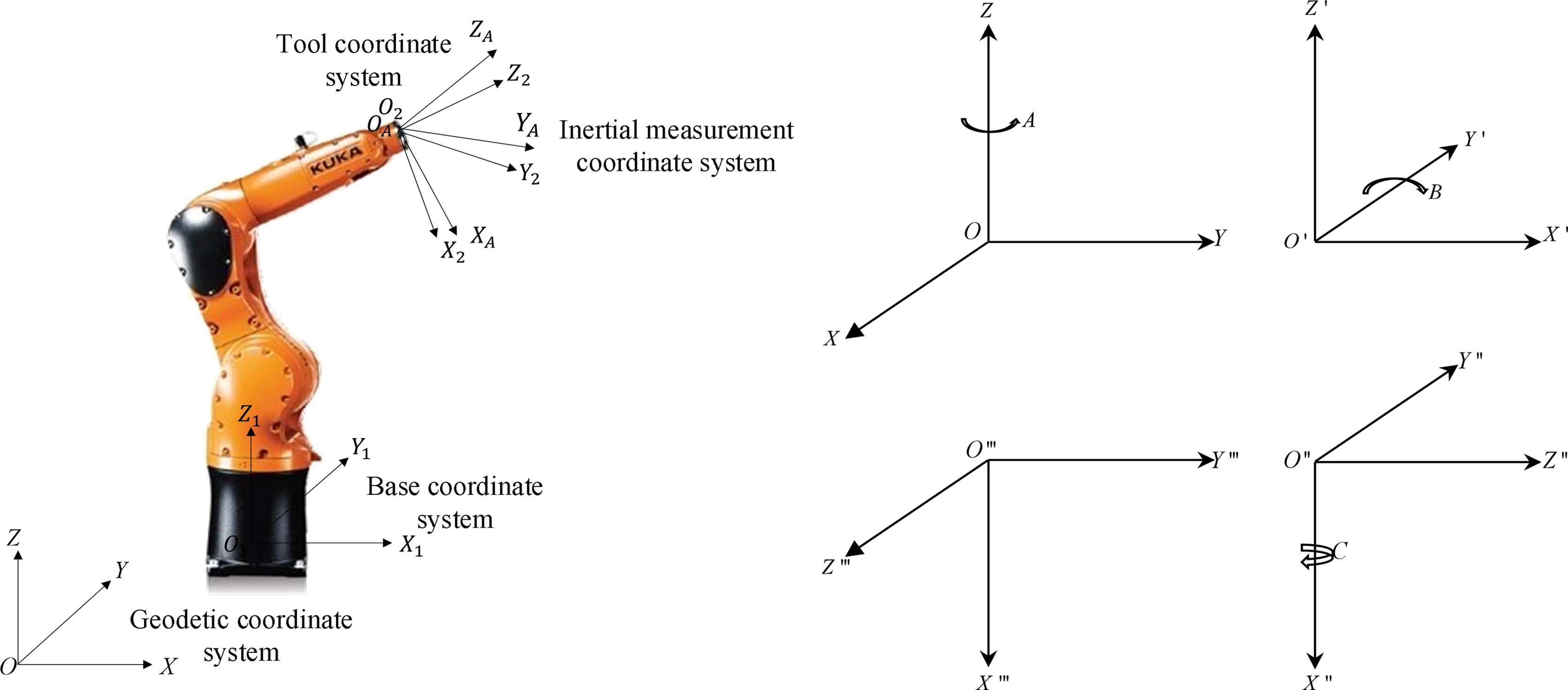
Figure 1. Rotation relationship diagram of an industrial robot.

The base coordinate system is consistent with the geodetic coordinate system. The tool coordinate system is a coordinate system with the tool central point of the industrial robot end-effector as the coordinate origin. The transformation relationship between the robot tool coordinate system and the base coordinate system is determined by the three angles A, B, and C, which, respectively, indicate the rotation angles on the Z-axis, Y-axis, and X-axis for the purpose of determining the attitude of the robot at any point in the robot workspace.

According to the Euler−Angle transformation relation, the rotation matrix of the robot tool coordinate and the base coordinate is

(1) \begin{equation} \textbf{R}_{\textbf{ZYX}}\left(A,B,C\right)=\left[\begin{array}{c@{\quad}c@{\quad}c} \cos A\cos B & \mathit{\cos }\ {\mathit A}\sin B\sin C-\sin A\sin C & \mathit{\cos } \ {\mathit A}\sin B\cos C+\sin A\sin C\\ \\[-7pt] \sin A\cos B & \mathit{\sin }\ {\mathit A}\sin B\sin C+\cos A\cos C & \mathit{\sin }\ {\mathit A}\sin B\cos C-\cos A\sin C\\ \\[-7pt] -\sin B & \cos B\sin C & \cos B\cos C \end{array}\right] \end{equation}

Using a set of Euler Angles to describe the transformation relationship between two coordinate systems is simple and easy to understand, but there are a lot of trigonometric function operations when using the angular velocity and acceleration information measured by IMU to solve the matrix. The quaternion method has the small computational complexity in the attitude calculation and is applicable to the whole attitude calculation, which cannot be well implemented with the Euler Angle method. Based on the characteristics of flexible attitude and low dynamic range of industrial robots, the quaternion method is selected to describe their attitudes [Reference Slamani, Nubiola and Bonev18–Reference Chiella, Teixeira and Pereira20]. According to the angular acceleration values of each axis output by the gyroscope, the quaternions are calculated and updated in real time with the quaternion differential equation. The quaternion is as follows:

(2) \begin{equation} {\bf{q}} = {q_0} + {q_1}\overrightarrow {\bf{i}} + {q_2}\overrightarrow {\bf{j}} + {q_3}\overrightarrow {\bf{k}} \end{equation}

where $\textbf{q}$ is attitude quaternion, $q_{0}$ , $q_{1}$ , $q_{2}$ , $q_{3}$ are real numbers, and $\overrightarrow {\bf{i}}$ , $\overrightarrow {\bf{j}}$ , $\overrightarrow {\bf{k}}$ are three orthogonal unit vectors.

According to the updated quaternion variables, attitude rotation matrix that was measured by inertial measurement system can be obtained as follows [Reference Ban, Ren and Chen21]:

(3) \begin{equation} {\textbf{R}}_{\textbf{n}}^{\textbf{b}}\left(q\right)=\left[\begin{array}{c@{\quad}c@{\quad}c} {q}_{0}^{2}+{q}_{1}^{2}-{q}_{2}^{2}-{q}_{3}^{2} & 2(q_{1}q_{2}-q_{0}q_{3}) & 2(q_{1}q_{3}+q_{0}q_{2})\\ \\[-7pt] 2(q_{1}q_{2}+q_{0}q_{3}) & {q}_{0}^{2}-{q}_{1}^{2}+{q}_{2}^{2}-{q}_{3}^{2} & 2(q_{2}q_{3}-q_{0}q_{1})\\ \\[-7pt] 2(q_{1}q_{3}-q_{0}q_{2}) & 2(q_{2}q_{3}+q_{0}q_{1}) & {q}_{0}^{2}-{q}_{1}^{2}-{q}_{2}^{2}+{q}_{3}^{2} \end{array}\right] \end{equation}

where n is the base coordinate system O₁-X₁Y₁Z₁, and b is the inertial measurement coordinate system O_A-X_AY_AZ_A.

2.2. Fourth-order Runge−Kutta algorithm

2.2.1. Fourth-order Runge−Kutta algorithm

Runge−Kutta method is a single-step algorithm widely applied in engineering. It does not require analytical linearization of discrete control equations and can perform local error control and adaptive time-stepping [Reference Wang, Zhai, He and Xu22]. Therefore, in this paper, the fourth-order Runge−Kutta algorithm is used in the calculation. By approximating the solution of the differential equation with the slope, the slopes of multiple points in the integral interval are predicted and weighted as the basis for the next point. In this way, a more accurate numerical integral calculation is constructed. Due to the noncommutability error of rotation, Runge−Kutta algorithm is suitable for the middle-low speed attitude motion [Reference Shi and Liu23]. For the application of inertial measurement of industrial robot, which usually moves at middle-low speed, the fourth-order Runge−Kutta algorithm can be used to calculate the attitude [Reference Liang, Xu and Huang24–Reference Luqiang, Yigang, Qiwu and Wei26].

The steps of the algorithm are described as follows:

1. 1. Assuming that the function y is sufficiently smooth, the first-order differential equation is

   (4) \begin{equation} y'=f(x,y) \end{equation}

2. 2. Taylor expansion of the function $y(x_{i+1})$ at $\textrm{x}_{i}$ is

   (5) \begin{equation} y\left(x_{i+1}\right)=y_{i}+hf'\left(x_{i},y_{i}\right)+\frac{h^{2}}{2!}f''\left(x_{i},y_{i}\right)+\cdots +O\left(h^{P}\right) \end{equation}

3. 3. When the order is larger than 2, the calculation of the higher order differentiation of the function is complex. The approximate formula can be constructed with the linear combination of the function values of $f(x,y)$ at some points. In this paper, with the fourth-order Runge−Kutta algorithm, the slope values at four points in $[x_{i},x_{i+1}]$ are calculated and then weighted as the average slope. Then, the fourth-order Runge−Kutta formula is constructed. This method has a fourth-order accuracy, and its error is $O(h^{5})$ .

$y_{i+1}$ is expressed as:

(6) \begin{equation} y_{i+1}=y_{i}+c_{1}K_{1}+c_{2}K_{2}+c_{3}K_{3}+c_{4}K_{4} \end{equation}

where K ₁, K ₂, K ₃, K ₄ are the function values at four different points, and they are shown as

\begin{align*} \begin{cases} K_{1}=hf(x_{i},y_{i})\\ \\[-8pt] K_{2}=hf(x_{i}+a_{2}h,y_{i}+b_{21}K_{1})\\ \\[-8pt] K_{3}=hf(x_{i}+a_{3}h,y_{i}+b_{31}K_{1}+b_{32}K_{2})\\ \\[-8pt] K_{4}=hf(x_{i}+a_{4}h,y_{i}+b_{41}K_{1}+b_{42}K_{2}+b_{43}K_{3}) \end{cases} \end{align*}

where c ₁, c ₂, c ₃, c ₄, a ₂, a ₃, a ₄, b ₂₁, b ₃₁, b ₃₂, b ₄₁, b ₄₂, b ₄₃ are undetermined coefficients.

K ₂, K ₃, and K ₄ are, respectively, expressed as the power series of h at point x _i and then substituted into linear equations. Then the obtained formulas are compared with the Taylor expansion of y(x _i+1 ) at point x _i . When the coefficients of h ₄ on the right sides of the obtained formulas and Taylor expansion are the same, a set of special solutions composed of a_i , b_ij , and c_j are obtained:

(7) \begin{align} \begin{cases} a_{2}=a_{3}=b_{21}=b_{32}=1/2\\ \\[-8pt] b_{31}=b_{41}=b_{42}=0\\ \\[-8pt] a_{4}=b_{43}=1\\ \\[-8pt] c_{1}=c_{4}=1/6\\ \\[-8pt] c_{2}=c_{3}=1/3 \end{cases} \end{align}

Substituting the calculated coefficients into Eq. (6), $y_{i+1}$ is expressed as

(8) \begin{equation} y_{i+1}=y_{i}+\frac{h}{6}\left(K_{1}+2K_{2}+2K_{3}+K_{4}\right) \end{equation}

where

\begin{align*} \begin{cases} K_{1}=f(x_{i},y_{i})\\ \\[-8pt] K_{2}=f\left(x_{i}+\frac{h}{2},y_{i}+\frac{K_{1}}{2}h\right)\\ \\[-8pt] K_{3}=f\left(x_{i}+\frac{h}{2},y_{i}+\frac{K_{2}}{2}h\right)\\ \\[-8pt] K_{4}=f(x_{i}+h,y_{i}+K_{3}h) \end{cases} \end{align*}

2.2.2. Inertial measurement attitude update and solution

With the fourth-order Runge−Kutta method, the attitude is solved. First, a quaternion differential equation needs to be established. Then, according to the strapdown inertial navigation theory, the quaternion differential equation is obtained as:

(9) \begin{equation} \left[\begin{array}{l} \dot{q}_{0}\\ \\[-8pt] \dot{q}_{1}\\ \\[-8pt] \dot{q}_{2}\\ \\[-8pt] \dot{q}_{3} \end{array}\right]=\frac{1}{2}\left[\begin{array}{c@{\quad}c@{\quad}c@{\quad}c} 0 & -\omega _{x} & -\omega _{y} & -\omega _{z}\\ \\[-8pt] \omega _{x} & 0 & -\omega _{z} & \omega _{y}\\ \\[-8pt] \omega _{y} & \omega _{z} & 0 & -\omega _{x}\\ \\[-8pt] \omega _{z} & -\omega _{y} & \omega _{x} & 0 \end{array}\right]\left[\begin{array}{l} q_{0}\\ \\[-8pt] q_{1}\\ \\[-8pt] q_{2}\\ \\[-8pt] q_{3} \end{array}\right] \end{equation}

where $\omega _{x},\omega _{y},\omega _{z}$ are, respectively, the angular velocities measured in X-, Y-, and Z-axes of the inertial measurement coordinate system by the gyroscope. Two matrices are, respectively, set as follows:

\begin{equation*} \textbf{q}(t)=[q_{0},q_{1},q_{2},q_{3}] \end{equation*}

\begin{equation*} \textbf{M}_{\boldsymbol{\omega }}\left(t\right)=\left[\begin{array}{c@{\quad}c@{\quad}c@{\quad}c} 0 & -\omega _{x}(t) & -\omega _{y}(t) & -\omega _{z}(t)\\ \\[-7pt] \omega _{x}(t) & 0 & -\omega _{z}(t) & \omega _{y}(t)\\ \\[-7pt] \omega _{y}(t) & \omega _{z}(t) & 0 & -\omega _{x}(t)\\ \\[-7pt] \omega _{z}(t) & -\omega _{y}(t) & \omega _{x}(t) & 0 \end{array}\right] \end{equation*}

$\textbf{M}_{\boldsymbol{\omega }}(t)$ is the angular velocity matrix at time t.

Then, the quaternion differential equation can be written as

(10) \begin{equation} \dot{\textbf{q}}\left(t\right)=\frac{1}{2}\textbf{M}_{\boldsymbol{\omega }}\left(t\right)\cdot \textbf{q}\left(t\right) \end{equation}

According to Eq. (9), $K_{i}(i=1-4)$ is obtained as

(11) \begin{align} \begin{cases} K_{1}=\frac{1}{2}\textbf{M}_{\boldsymbol{\omega }}\left(t\right)\textbf{q}\left(t\right)\\ \\[-8pt] K_{2}=\frac{1}{2}\textbf{M}_{\boldsymbol{\omega }}\left(t+\frac{T}{2}\right)\left[\textbf{q}\left(t\right)+\frac{K_{1}}{2}T\right]\\ \\[-8pt] K_{3}=\frac{1}{2}\textbf{M}_{\boldsymbol{\omega }}\left(t+\frac{T}{2}\right)\left[\textbf{q}\left(t\right)+\frac{K_{2}}{2}T\right]\\ \\[-8pt] K_{4}=\frac{1}{2}\textbf{M}_{\boldsymbol{\omega }}\left(t+T\right)\left[\textbf{q}\left(t\right)+K_{3}T\right] \end{cases} \end{align}

where T is the sampling interval.

According to the fourth-order Runge−Kutta formula, the inertial measurement attitude quaternion is updated as

(12) \begin{equation} \textbf{q}\left(t+T\right)=\textbf{q}\left(t\right)+\frac{T}{6}\left[K_{1}+2K_{2}+2K_{3}+K_{4}\right] \end{equation}

Substituting the inertial measurement attitude quaternions into Eq. (3), the robot end-effector attitude rotation matrix ${\textbf{R}}_{\textbf{n}}^{\textbf{b}}(q)$ measured by the inertial measurement system can be obtained.

2.3. Other algorithms

In the inertial measurement, we commonly used attitude updating algorithms that include incremental Picard algorithm, Rotation Vector method, Digital Integration algorithm, and Accurate Numerical Solution method [Reference Chen27]. Picard algorithm and Rotation Vector method were applied to calculate the attitude by using the same measurement data in order to analyze the characteristics and applicability of the attitude updating algorithm and compared the results with fourth-order Runge−Kutta algorithm. Picard algorithm is essentially a monad rotation vector algorithm, which is suitable for low speed motion. The Rotation Vector method can be used to solve the high-speed motion due to the nonommutativity error was compensated in the updating process. However, when the sensor output is not an angular increment, such as calculating with the angular velocity output by the gyroscope will cause a larger error.

2.3.1. Picard algorithm

The basic process of incremental Picard algorithm is as follows:

First, the quaternion differential equation (Eq. 10) can be solved by Picard series:

(13) \begin{equation} \textbf{q}\left(t_{k+1}\right)=e^{\frac{1}{2}{{\int }_{{t_{k}}}}^{t_{k+1}}\textbf{M}_{\boldsymbol{\omega }}(t)dt}\textbf{q}\left(t_{k}\right) \end{equation}

Making $\boldsymbol{\Delta \Theta }={\int }_{t_{k}}^{t_{k+1}}\textbf{M}_{\boldsymbol{\omega }}(t)dt$

\begin{equation*} \boldsymbol{\Delta \Theta }={\int }_{t_{k}}^{t_{k+1}}\left[\begin{array}{c@{\quad}c@{\quad}c@{\quad}c} 0 & -{\omega }_{nbx}^{b} & -{\omega }_{nby}^{b} & -{\omega }_{nbz}^{b}\\ \\[-7pt] {\omega }_{nbx}^{b} & 0 & {\omega }_{nbz}^{b} & -{\omega }_{nby}^{b}\\ \\[-7pt] {\omega }_{nby}^{b} & -{\omega }_{nbz}^{b} & 0 & {\omega }_{nbx}^{b}\\ \\[-7pt] {\omega }_{nbz}^{b} & {\omega }_{nby}^{b} & -{\omega }_{nbx}^{b} & 0 \end{array}\right]\textrm{d}t=\left[\begin{array}{c@{\quad}c@{\quad}c@{\quad}c} 0 & -\Delta \theta _{x} & -\Delta \theta _{y} & -\Delta \theta _{z}\\ \\[-7pt] \Delta \theta _{x} & 0 & \Delta \theta _{z} & -\Delta \theta _{y}\\ \\[-7pt] \Delta \theta _{y} & -\Delta \theta _{z} & 0 & \Delta \theta _{x}\\ \\[-7pt] \Delta \theta _{z} & \Delta \theta _{y} & -\Delta \theta _{x} & 0 \end{array}\right] \end{equation*}

where $\Delta\theta _{x} \Delta\theta _{y} \Delta\theta _{z}$ are the angular increments of the industrial robot in the three axes during the timing sampling; ${\omega }_{nbx}^{b} {\omega }_{nby}^{b} {\omega }_{nbz}^{b}$ are the three axial angular velocities of industrial robot in the inertial measurement coordinate system.

Making Taylor expansion of Eq. (13) and sorting out it can obtain:

(14) \begin{equation} \textbf{q}\left(\textrm{t}_{k+1}\right)=\left(\textbf{I}\cos \frac{\Delta \theta }{2}+\boldsymbol{\Delta \Theta }\frac{\sin \frac{\Delta \theta }{2}}{\Delta \theta }\right)\textbf{q}\left(\textrm{t}_{k}\right) \end{equation}

where $\Delta \theta$ is the angular increment, including $\Delta \theta _{x} \Delta\theta _{y} \Delta\theta _{z}$ ; $\textbf{q}$ is quaternion variable, t is the time constant, $\boldsymbol{\Delta \Theta }$ is the coefficient matrix, and $\textbf{I}$ is unit matrix.

The corresponding quaternion variables can be obtained from the angular increment of industrial robot at each moment. Then the next moment quaternion can be obtained by iterating through formula (14). Finally, the quaternion attitude rotation matrix can be obtained.

2.3.2 Rotation vector method

The rotation vector indicates that the dynamic coordinate system rotates in space around the initial fixed coordinate system attached to the rigid body. This rotation relationship is expressed by an equivalent rotation vector, and it is equivalent to a dynamic coordinate system rotating an angle around the direction of an equivalent rotation vector. The equivalent rotation vector can be solved through angular increment and then updates the direction cosine matrix or quaternion by the equivalent rotation vector.

First, according to the rotation of the coordinate system to obtain the relationship between the equivalent rotation vector and the attitude change quaternion:

(15) \begin{equation}\left\{ \begin{array}{l}{\bf{q}}({t_{k + 1}}) = {\bf{q}}({t_k}) \otimes {\bf{q}}(h)\\[4pt]{\bf{q}}(h) = \cos \left( {\frac{{\overrightarrow {\boldsymbol{\Phi }} }}{2}} \right) + \frac{{\overrightarrow {\boldsymbol{\Phi }} }}{{\left| {\overrightarrow {\boldsymbol{\Phi }} } \right|}}\sin \left( {\frac{{\overrightarrow {\boldsymbol{\Phi }} }}{2}} \right)\end{array} \right.\end{equation}

where $\textbf{q}(t_{k+1})$ is the attitude quaternion from $t_{k}$ to $t_{k+1}, \textbf{q}(h)$ is the attitude change quaternion between these two moments: $t_{k}$ ~ $t_{k+1}, h=t_{k+1}-t_{k}, \overrightarrow {\bf{\Phi }}$ is the equivalent rotation vector, $\otimes$ denotes quaternion multiplication.

Since attitude update only pays attention to the rotation vector in the time from the start moment to the end moment, the approximate rotation vector differential equation in engineering can be derived:

(16) \begin{equation}\mathop {\overrightarrow {\bf{\Phi }} }\limits^ \bullet = {\bf{\omega }}_{{\bf{nb}}}^{\bf{b}} + \frac{1}{2}\overrightarrow {\bf{\Phi }} \times {\bf{\omega }}_{{\bf{nb}}}^{\bf{b}} + \frac{1}{{12}}\overrightarrow {\bf{\Phi }} \times \left( {\overrightarrow {\bf{\Phi }} \times {\bf{\omega }}_{{\bf{nb}}}^{\bf{b}}} \right) \end{equation}

where $\mathop {\overrightarrow {\bf{\Phi }} }\limits^ \bullet$ denotes an approximate rotation vector, ${\boldsymbol{\omega }}_{\textbf{nb}}^{\textbf{b}}$ is the angular velocity of the gyroscope in the three axes, including ${\omega }_{nbx}^{b} {\omega }_{nby}^{b} {\omega }_{nbz}^{b}$ ; n is base coordinate system O₁-X₁Y₁Z₁, and b denotes the inertial measurement coordinate system O_A-X_AY_AZ_A.

Supposing that the equivalent rotation vector caused by angular position change in time $\left[t_{k},t_{k+1}\right]$ is $\overrightarrow {\bf{\Phi }} \left( h \right)$ , sampling n times at the same time interval can obtain n angle increments. Taking n = 4 as an example, the four-subsample formula of the rotation vector is

(17) \begin{align} \overrightarrow {\bf{\Phi }} \left( h \right)&=\Delta \theta _{1}+\Delta \theta _{2}+\Delta \theta _{3}+\Delta \theta _{4}+\frac{736}{945}\left(\Delta \theta _{1}\times \Delta \theta _{2}+\Delta \theta _{3}\times \Delta \theta _{4}\right)+\cdots \nonumber\\ & \quad \frac{334}{945}\left(\Delta \theta _{1}\times \Delta \theta _{3}+\Delta \theta _{2}\times \Delta \theta _{4}\right)+\frac{526}{945}\Delta \theta _{1}\times \Delta \theta _{4}+\frac{526}{945}\Delta \theta _{2}\times \Delta \theta _{3} \end{align}

$\Delta \theta _{1} \Delta \theta _{2} \Delta \theta _{3} \Delta \theta _{4}$ are the angular increment of the rotation vector in four subtime periods.

After the rotation vector was calculated, the corresponding attitude change quaternions could be obtained according to the Eq. (15). Then the corresponding attitude rotation matrix can be obtained according to the attitude change quaternions.

Aiming at the application scenarios of industrial robots work in middle-low speed situations and the characteristic that the output of the inertial sensor is angular velocity, we adopt the fourth-order Runge−Kutta algorithm to solve the attitude.

3.1. Selection of gyroscope and accelerometer

In this paper, the gyroscope [Reference Qi, Zhang, Zhang, Zheng and Chen28] and accelerometer [Reference Qi, Chen, Zhang, Zhang, Wang and Tan29] were used to measure the angular velocity and linear acceleration at the end of an industrial robot. Gyroscope can be divided into mechanical gyroscope and optical gyroscope according to the principle. In this paper, the optical fiber gyroscope is selected to measure angular velocity. It is an improved type of laser gyroscope. Due to the use of optical fiber ring the optical path difference during rotation is greatly increased, so as to improve the detection accuracy. Accelerometers are divided into pendulum and non pendulum accelerometers according to the principle. We used the quartz flexible accelerometer in this paper. The quartz material can effectively reduce the influence of temperature and the material performance is stable, which is conducive to the improvement of accuracy.

Table I. HT-120 main performance indicators.

Figure 2. Fiber-optic gyroscope HT-120.

The selected single-axis fiber-optic gyroscope (HT-120) is shown in Fig. 2. The measurement is based on Sagnac effect principle. The gyroscope has the advantages of high zero-bias stability, minimal random walk coefficient, high accuracy, and resistance to temperature change and electromagnetic interference. Its main performance indicators are shown in Table I.

The selected quartz flexible accelerometer (JHT-I-A) is shown in Fig. 3. When the sensor moves, the internal detection unit position is changed. The position change is converted into the current change and then amplified. The acceleration can be measured to calculate the current value. Its main performance indicators are shown in Table II.

Table II. Accelerometer JHT-I-A main performance indicators.

The acceleration components and angular velocity components on the X-axis, Y-axis, and Z-axis of the industrial robot end-effector were measured with three single-axis accelerometers and fiber-optic gyroscopes, respectively. According to the size and wiring method of the selected inertial device, an inertial device connector was designed to orthogonally install the gyroscope and accelerometer onto the end of the industrial robot. Therefore, an inertial measurement system was formed to collect the motion parameters of the robot end-effector. In order to ensure the rigidity and the proper weight of the connector, the connector was composed of six aluminum alloy square plates with six mounting holes and locating holes (Fig. 4).

Figure 3. Accelerometer JHT-I-A.

Figure 4. Installation diagram of inertial components.

The constructed inertial measurement system was installed on the flange at the end of the industrial robot with screws. The attitude measurement system platform is shown in Fig. 5. Since the accelerometer outputs a weak voltage signal and its central frequency is 3 kHz, it can be known that the sampling frequency of the single channel of the acquisition card is more than 6 kHz at least according to the sampling theorem. The fiber-optic gyroscope outputs digital signals and adopts RS422 serial port communication mode. The communication baud rate of the acquisition card needs to be matched with the fiber-optic gyroscope to reach 614.4 kps. Therefore, we chose the USB-6002 analog signal acquisition card and USB-422/4 digital signal acquisition card of NI company. The signals of the gyroscopes and accelerometers were synchronously transmitted to the upper computer software which developed based on LabVIEW platform via the data acquisition card and the actual attitude of the industrial robot end-effector was obtained after processing with the software.

Figure 5. Attitude measurement system.

4.1. Calibration of the inertial device

4.1.1. Accelerometer calibration

In this paper, the accelerometer was first calibrated roughly and then accurately calibrated to obtain the more accurate error coefficient. First, three accelerometers were connected orthogonally to each other and placed on a horizontal plane. Then, the sensitive axis direction of each accelerometer on X-, Y-, and Z-axes, respectively, pointed to the sky and the earth, and the output voltage of each accelerometer was collected.

Take the X-axis pointing to the sky as an example—the error equations are:

(18) \begin{align} \textrm{g}&=B_{\textrm{x}}+S_{x}V_{\textrm{x}1}+E_{xy}V_{\textrm{y}1}+E_{xz}V_{\textrm{z}1}\nonumber\\[3pt] 0&=B_{y}+E_{yx}V_{\textrm{x}1}+S_{y}V_{\textrm{y}1}+E_{yz}V_{\textrm{z}1} \nonumber \\[3pt]0&=B_{\textrm{z}}+E_{zx}V_{\textrm{x}1}+E_{zy}V_{\textrm{y}1}+S_{z}V_{\textrm{z}1} \end{align}

where

$\textrm{g}$ —Acceleration of gravity;

$B_{i}(i={\mathit x} y z)$ —Accelerometer zero offset;

$S_{i}(i={\mathit x} y z)$ —Accelerometer scale factor;

$V_{ij}(i={\mathit x} y z,j=1-6)$ —Output voltage of each accelerometer in X-, Y-, and Z-axes, respectively, at six positions obtained through rough calibration; j = 1−6, respectively, indicate six cases: X-axis points to the sky; X-axis points to the earth; Y-axis points to the sky; Y-axis points to the earth; Z-axis points to the sky; and Z-axis points to the earth;

$E_{ij}(i={\mathit x} {\mathit y} z,j={\mathit x} {\mathit y} z,i\neq j)$ ——Installation error factor.

Three equations for each coordinate axis were established, and six attitudes were selected for the measurements. The coefficient term was solved by the least square method so as to obtain the rough calibration results.

(19) \begin{equation} \left[\begin{array}{c@{\quad}c@{{\quad}}c} B_{x0} & B_{y0} & B_{z0}\\ \\[-7pt] S_{x0} & E_{yx0} & E_{zx0}\\ \\[-7pt] E_{xy0} & S_{y0} & E_{zy0}\\ \\[-7pt] E_{xz0} & E_{yz0} & S_{z0} \end{array}\right] \end{equation}

where the subscript “0” represents the result of the rough calibration of the accelerometers.

On the basis of rough calibration results, the accurate calibration was performed after the accelerometer group was placed on the precision turntable. Figure 6 shows an experimental device for accurate calibration. The X-, Y-, and Z- axes were adjusted according to the four directions: vertically upward direction, the oblique direction along the angle of 45° with the horizontal plane, vertically downward direction, and the oblique direction along the angle of 135° with the horizontal plane. The output voltages of 12 attitudes were measured.

Figure 6. Accelerometer calibration experiment.

The square of gravitational acceleration is equal to the vectorial summation of the square of the acceleration in each axis under static conditions:

(20) \begin{equation} \textrm{g}^{2}={A}_{x}^{2}+{A}_{y}^{2}+{A}_{z}^{2} \end{equation}

where

$A_{x} A_{y} A_{z}$ —Each axial acceleration.

Taking the X-axis as an example, the square sum of the left and right sides of Eq. (18) is calculated as

(21) \begin{align} \textrm{g}^{2}&={A}_{x}^{2}+{A}_{y}^{2}+{A}_{z}^{2} \nonumber \\[3pt] &=\left(B_{x}+S_{x}\overline{V_{x1}}+E_{xy}\overline{V_{y1}}+E_{xz}\overline{V_{z1}}\right)^{2}+\left(B_{y}+E_{yx}\overline{V_{x1}}+S_{y}V_{\textrm{y}1}+E_{yz}\overline{V_{z1}}\right)^{2}\nonumber \\[3pt] &\quad +\left(B_{z}+E_{zx}\overline{V_{x1}}+E_{zy}\overline{V_{y1}}+S_{z}\overline{V_{z1}}\right)^{2} \end{align}

where

$B_{i}(i={\mathit x} y z)$ —Each accelerometer zero offset;

$E_{ij}(i={\mathit x} {\mathit y} z,j={\mathit x} {\mathit y} z,i\neq j)$ —Accelerometer installation error of each axis;

$\overline{V_{ij}}\left(i={\mathit x} y z,j=1-12\right)$ —The average value of the output voltages of each accelerometer in X-, Y-, and Z-axes at 12 positions obtained after accurate calibration.

Substituting 12 groups of average voltage values ( $\overline{V_{ij}}$ ) of measurements into Eq. (21) gives:

(22) \begin{equation} \begin{array}{l} f_{1}=\left(B_{x}+S_{x}\overline{V_{x1}}+E_{xy}\overline{V_{y1}}+E_{xz}\overline{V_{z1}}\right)^{2}+\cdots +\left(B_{\textrm{z}}+E_{zx}\overline{V_{x1}}+E_{zy}\overline{V_{y1}}+S_{z}\overline{V_{z1}}\right)^{2}-\textrm{g}^{2}=0\\ \\[-7pt] \begin{array}{l} \end{array}\vdots \begin{array}{c@{\quad}c} & \begin{array}{l} \end{array}\vdots \end{array}\begin{array}{l} \end{array}\begin{array}{l} \begin{array}{l} \begin{array}{l} \end{array} \end{array} \end{array}\begin{array}{c@{\quad}c} & \begin{array}{l} \end{array}\vdots \end{array}\begin{array}{l} \begin{array}{l} \begin{array}{l} \end{array} \end{array} \end{array}\begin{array}{l} \end{array}\begin{array}{c@{\quad}c} \begin{array}{l} \end{array} & \vdots \end{array}\begin{array}{l} \begin{array}{l} \begin{array}{l} \end{array} \end{array} \end{array}\begin{array}{l} \end{array}\begin{array}{c@{\quad}c} & \end{array}\begin{array}{c@{\quad}c} \begin{array}{l} \end{array} & \vdots \end{array}\begin{array}{l} \begin{array}{l} \begin{array}{l} \end{array} \end{array} \end{array}\begin{array}{l} \end{array}\begin{array}{c@{\quad}c} & \end{array}\begin{array}{c@{\quad}c} \begin{array}{l} \end{array} & \vdots \end{array}\\ \\[-7pt] f_{12}=\left(B_{x}+S_{x}\overline{V_{x12}}+E_{xy}\overline{V_{y12}}+E_{xz}\overline{V_{z12}}\right)^{2}+\cdots +\left(B_{\textrm{z}}+E_{zx}\overline{V_{x12}}+E_{zy}\overline{V_{y12}}+S_{z}\overline{V_{z12}}\right)^{2}-\textrm{g}^{2}=0 \end{array} \end{equation}

Then, the nonlinear equations were solved with the Newton iteration method. The results of rough calibration, as the initial value, were submitted into the above equations. Then through Taylor expansion of Eq. (22), the following equations are obtained:

(23) \begin{equation} \begin{array}{l} f_{1}=f_{1}\left(B_{x0},\cdots,S_{z0}\right)+\dfrac{\partial f_{1}}{\partial B_{x}}\Big| _{{B_{x0}}}\left(B_{x}-B_{x0}\right)+\cdots +\dfrac{\partial f_{1}}{\partial S_{z}}\Big| _{{S_{z0}}}\left(S_{z}-S_{z0}\right)=0\\ \\[-7pt] \begin{array}{l} \end{array}\vdots \begin{array}{c@{\quad}c} & \begin{array}{l} \end{array}\vdots \end{array}\begin{array}{l} \end{array}\begin{array}{l} \begin{array}{l} \begin{array}{l} \end{array} \end{array} \end{array}\begin{array}{c@{\quad}c} & \begin{array}{l} \end{array}\vdots \end{array}\begin{array}{l} \begin{array}{l} \begin{array}{l} \end{array} \end{array} \end{array}\begin{array}{l} \end{array}\begin{array}{c@{\quad}c} \begin{array}{l} \end{array} & \vdots \end{array}\begin{array}{l} \begin{array}{l} \begin{array}{l} \end{array} \end{array} \end{array}\begin{array}{l} \end{array}\begin{array}{c@{\quad}c} & \end{array}\begin{array}{c@{\quad}c} \begin{array}{l} \end{array} & \vdots \end{array}\begin{array}{l} \begin{array}{l} \begin{array}{l} \end{array} \end{array} \end{array}\begin{array}{l} \end{array}\begin{array}{c@{\quad}c} & \end{array}\begin{array}{c@{\quad}c} \begin{array}{l} \end{array} & \vdots \end{array}\\ \\[-7pt] f_{12}=f_{12}\left(B_{x0},\ldots,S_{z0}\right)+\dfrac{\partial f_{12}}{\partial B_{x}}\Big| _{{B_{x0}}}\left(B_{x}-B_{x0}\right)+\cdots +\dfrac{\partial f_{12}}{\partial S_{z}}\Big| _{{S_{z0}}}\left(S_{z}-S_{z0}\right)=0 \end{array} \end{equation}

The optimal solution was approached gradually by multiple iterations, and finally the error coefficient was controlled within a certain range. In order to reduce the interference of random noise in the data collection process, sufficient sampling time should be guaranteed for the data collection in each attitude and more testing attitudes should be selected. The calibration results of the accelerometer error term coefficient are shown in Table III.

Table III. Accelerometer error term coefficient calibration result.

4.1.2. Scale factor calibration of the gyroscope

The single-axis fiber-optic gyroscope was installed on a high-precision turntable in such a proper way that the sensitive axis was parallel to the spindle of the turntable in the initial position (Fig. 7). The high-precision turntable was controlled to rotate around the spindle at a certain angular rate. An improper input angular rate might cause the nonlinear output, thus leading to the inaccurate calibration result. The angular rate used in this paper was between 10°/s and 100°/s. In order to eliminate the influence of the earth rotation on the motion of the turntable, it is necessary to control the turntable to rotate integral circles in each motion. Otherwise, the horizontal component of the earth rotation would increase the error. During the experiment, it was necessary to precisely control the turntable in order to ensure the accuracy of gyroscope calibration results. The calibration results of the gyroscope scale factors are shown in Table IV.

Table IV. Fiber-optic gyroscope scale factor calibration result.

Figure 7. Fiber-optic gyroscope calibration experiment.

4.2. Installation error compensation of the inertial measurement system

In this study, the inertial measurement system was composed of three single-axis accelerometers and three single-axis fiber-optic gyroscopes. It is necessary to ensure that the sensitive axes are orthogonal to each other during the installation process. However, due to the manufacturing error of the connector and the installation error of the inertial component group, it is difficult to ensure that the sensors are perfectly orthogonally installed at the center of the industrial robot end-effector. Therefore, it is necessary to calibrate the whole inertial measurement system and compensate its installation error.

The installation error calibration steps of the inertial measurement system were introduced as follows:

1. 1. Install three single-axis accelerometer sensors orthogonally onto the inertial component connection device and connect them to the data acquisition card USB-6002;

2. 2. Fix the inertial component connection device onto the industrial robot end-effector;

3. 3. Select the tool coordinate system in the manual mode of the industrial robot (the origin of the coordinate system is the center point of the end flange of the industrial robot), control the robot to move linearly along the X-, Y-, and Z-axes of the tool coordinate system and measure the voltage output values of the accelerometers in real time;

The direction of each coordinate axis of the industrial robot in the inertial measurement system coordinate system can be expressed with its unit vector:

(24) \begin{align}\overrightarrow {{{\bf{e}}_{{\bf{2xb}}}}} = {\left[ {\begin{array}{*{20}{c}}{{e_{2xbx}}}&{{e_{2xby}}}&{{e_{2xbz}}}\end{array}} \right]^T} = \frac{{{{\left[ {\begin{array}{*{20}{c}}{{a_{x1}} - {a_{x0}}}&{{a_{y1}} - {a_{y0}}}&{{a_{z1}} - {a_{z0}}}\end{array}} \right]}^T}}}{{\sqrt {{{({a_{x1}} - {a_{x0}})}^2} + {{({a_{y1}} - {a_{y0}})}^2} + {{({a_{z1}} - {a_{z0}})}^2}} }} \nonumber \\[3pt] \overrightarrow {{{\bf{e}}_{{\bf{2yb}}}}} = {\left[ {\begin{array}{*{20}{c}}{{e_{2ybx}}}&{{e_{2yby}}}&{{e_{2ybz}}}\end{array}} \right]^T} = \frac{{{{\left[ {\begin{array}{*{20}{c}}{{a_{x2}} - {a_{x0}}}&{{a_{y2}} - {a_{y0}}}&{{a_{z2}} - {a_{z0}}}\end{array}} \right]}^T}}}{{\sqrt {{{({a_{x2}} - {a_{x0}})}^2} + {{({a_{y2}} - {a_{y0}})}^2} + {{({a_{z2}} - {a_{z0}})}^2}} }} \nonumber \\[3pt] \overrightarrow {{{\bf{e}}_{{\bf{2zb}}}}} = {\left[ {\begin{array}{*{20}{c}}{{e_{2zbx}}}&{{e_{2zby}}}&{{e_{2zbz}}}\end{array}} \right]^T} = \frac{{{{\left[ {\begin{array}{*{20}{c}}{{a_{x3}} - {a_{x0}}}&{{a_{y3}} - {a_{y0}}}&{{a_{z3}} - {a_{z0}}}\end{array}} \right]}^T}}}{{\sqrt {{{({a_{x3}} - {a_{x0}})}^2} + {{({a_{y3}} - {a_{y0}})}^2} + {{({a_{z3}} - {a_{z0}})}^2}} }}\end{align}

where

$\overrightarrow {{{\bf{e}}_{{\bf{2xb}}}}} \overrightarrow {{{\bf{e}}_{{\bf{2yb}}}}} \overrightarrow {{{\bf{e}}_{{\bf{2zb}}}}}$ —Direction vectors of the robot tool coordinate X-, Y-, and Z-axes in the inertial measurement coordinate system;

$a_{x0} a_{y0} a_{z0}$ —The acceleration values in the three axis directions before the robot moves;

$a_{x1} a_{y1} a_{z1}$ —The accelerometer readings after the robot moves along the X-axis;

$a_{x2} a_{y2} a_{z2}$ —The accelerometer readings after the robot moves along the Y-axis;

$a_{x3} a_{y3} a_{z3}$ —The accelerometer readings after the robot moves along the Z-axis.

Therefore, the rotation matrix from the tool coordinate system to the inertial device coordinate system can be obtained as

(25) \begin{equation} {\textbf{R}}_{\textbf{2}}^{\textbf{b}}=\left[\begin{array}{c@{\quad}c@{\quad}c} e_{2xA} & e_{2yA} & e_{2zA} \end{array}\right]^{T} \end{equation}

where b is the inertial measurement coordinate system O_A-X_AY_AZ_A, and 2 is the robot tool coordinate system O₂-X₂Y₂Z₂.

Through the transformation of the matrix, the installation error of inertial measurement system can be compensated. In this way, the installation error of the whole measurement system is corrected and finally the attitude matrix R of the industrial robot is obtained as

(26) \begin{equation} \textbf{R}={\textbf{R}}_{\textbf{n}}^{\textbf{b}}{\textbf{R}}_{\textbf{2}}^{\textbf{b}} \end{equation}

By comparing Eq. (1) and $\textbf{R}$ , the attitude angles A, B, and C of the robot end-effector are

(27) \begin{align} \begin{cases} A=\arctan \frac{r_{21}}{r_{11}}\\ \\[-7pt] B=\arctan \frac{r_{31}}{\sqrt{{r}_{11}^{2}+{r}_{21}^{2}}}\\ \\[-7pt] C=\arctan \frac{r_{32}}{r_{33}} \end{cases} \end{align}

where $r_{\textrm{ij}}$ is the element of row i and column j in the attitude matrix $\textbf{R}$ .

5.1. Repetitive experiment

To verify the repeatability precision of the inertial measurement system, eight points in the motion space of the robot were selected as the testing points. Under 50% of the rated load of the industrial robot, the end of the robot was controlled to move at a speed of 50% for 30 times. The attitude measurement data of point P₁ in 30 times are shown in Table V.

Table V. Attitude measurement results of P₁.

The mean attitude of point P₁ was calculated as (0.136°, 59.980°, 0.079°), and the uncertainties were, respectively, $\sigma _{A}$ = 0.015°, $\sigma _{B}$ = 0.006°, and $\sigma _{C}$ = 0.008°. The measurement results showed good repeatability and met the repeatability requirements of the robot attitude measurement.

The attitude measurement results at points P₁ to P₈ are shown in Table VI. The measurement uncertainty is less than 0.026°, indicating that the measurement repeatability at different positions in the measurement space is consistent. The measurement repeatability of each point is satisfactory.

Table VI. P₁−P₈ attitude measurement results.

The difference between the attitude data measured with the inertial measurement system and the theoretical data was less than 0.140°. It was mainly caused by measurement errors and control errors of the robot. In this study, in order to analyze the measurement error of inertial measurement system, the measurement data of the inertial measurement system were compared with the data of the high-precision measuring instrument, Leica laser tracker [Reference Chen, Mendoza and Griffith30,Reference Chen, Joffre and Avitabile31].

5.2. Measurement comparison experiment with laser tracker

In the measurement comparison experiment, the laser tracker coordinate system and the robot base coordinate system should be transformed into the global coordinate system. However, the coordinate system transformation error would be necessarily introduced in the transformation. In this paper, the end attitude of the robot was measured with a laser tracker and then the attitude measurement accuracy could be compared without solving the coordinate system transformation matrix. The method is introduced below.

First, the reflective target ball of the laser tracker was fixed at the center of the flange, and the robot base coordinate system was selected as the reference for programing. The robot was controlled to move 50 cm, respectively, along the X-, Y-, and Z- axes of the base coordinate system, and a series of discrete points along each coordinate axis of the base coordinate system could be obtained by using the laser tracker: $x_{bxi}, y_{bxi}, z_{bxi}$ , $x_{byi}, y_{byi}, z_{byi}$ , $x_{bzi}, y_{bzi}, z_{bzi}$ .

Then the robot tool coordinate system was selected as the reference for programing. The robot was controlled to move 50 cm, respectively, along the X-, Y-, and Z-axes of the tool coordinate system, and a series of discrete points along each coordinate axis of the tool coordinate system could be obtained with the laser tracker: $x_{txi}, y_{txi}, z_{txi}$ , $x_{tyi}, y_{tyi}, z_{tyi}$ , $x_{tzi}, y_{tzi}, z_{tzi}$ .

The distribution of the data measured by the laser tracker moving along the axes in different coordinate systems is shown in Fig. 8.

Figure 8. Spatial analyzer software measurement diagram of robot’s two coordinate systems.

Linear fitting was performed with the six sets of discrete point data, and its space linear equations were obtained by regression fitting so as to get the unit vectors in the X-, Y-, and Z-axes of the base coordinate system and the tool coordinate system. The robot tool coordinate system is defined as O₂-X₂Y₂Z_2, and the robot base coordinate system is defined as O₁-X₁Y₁Z₁. It is assumed that the unit vectors of the coordinate axis of the robot base coordinate system measured with the laser tracker are v _x , v _y , and v _z . The unit vectors of the coordinate axes of the robot tool coordinate system are n, o, and a.

The projection of n, o, and a in the robot base coordinate system can form the robot end-effector attitude matrix measured by the laser tracker. The attitude matrix $\textbf{R}_{\textbf{L}}$ obtained from the laser tracker is expressed as

(28) \begin{equation} \textbf{R}_{\textbf{L}}=\left(\begin{array}{c@{\quad}c@{\quad}c} r_{{L_{11}}} & r_{{L_{12}}} & r_{{L_{13}}}\\ \\[-7pt] r_{{L_{21}}} & r_{{L_{22}}} & r_{{L_{23}}}\\ \\[-7pt] r_{{L_{31}}} & r_{{L_{32}}} & r_{{L_{33}}} \end{array}\right) \end{equation}

where

\begin{equation} \left\{\begin{array}{c@{\quad}c@{\quad}c} r_{{L_{11}}}=\dfrac{n\cdot v_{x}}{\left| v_{x}\right| } & r_{{L_{21}}}=\dfrac{n\cdot v_{y}}{\left| v_{y}\right| } & r_{{L_{31}}}=\dfrac{n\cdot v_{z}}{\left| v_{z}\right| }\\ \\[-7pt] r_{{L_{21}}}=\dfrac{o\cdot v_{x}}{\left| v_{x}\right| } & r_{{L_{22}}}=\dfrac{o\cdot v_{y}}{\left| v_{y}\right| } & r_{{L_{23}}}=\dfrac{o\cdot v_{z}}{\left| v_{z}\right| }\\ \\[-7pt] r_{{L_{31}}}=\dfrac{a\cdot v_{x}}{\left| v_{x}\right| } & r_{{L_{32}}}=\dfrac{a\cdot v_{y}}{\left| v_{y}\right| } & r_{{L_{33}}}=\dfrac{a\cdot v_{z}}{\left| v_{z}\right| } \end{array}\right. \end{equation}

According to the coordinate transformation sequence of the robot, the attitude angle of the robot end-effector can be obtained through formula (27).

Five spatial poses in the robot motion space were selected, and the attitude of the industrial robot end-effector was measured with the laser tracker. The measured results were compared with those of the inertial measurement system to verify the precision and accuracy of the inertial measurement method. The measurement results of the laser tracker and inertial measurement system are shown in Table VII. Therefore, the measurement results are in good agreement with the results of external high-precision measuring equipment.

Table VII. Experimental results comparison.

5.3. Comparison of solution results of different algorithms

In order to analyze the accuracy of the fourth-order Runge–Kutta algorithm, fourth-order Runge−Kutta algorithm, Picard algorithm, and Rotation vector method were, respectively, used to solve the measurement data of point P₁ in Section 5.1, and these results were compared with the attitude measured by the laser tracker. The accuracy of different algorithms was analyzed, and the comparison results of point P₁ are shown in Table VIII.

Table VIII. The error comparison of the three algorithms.

From Table VIII, it can be seen that for the angle A and angle B, fourth-order Runge−Kutta algorithm has the smallest average error and uncertainty, followed by rotation vector method and the error of Picard algorithm is the largest. For the angle C, rotation vector method has the smallest average error and uncertainty, followed by fourth-order Runge−Kutta algorithm, and the Picard algorithm is the largest. The difference of error between the fourth-order Runge−Kutta and the rotation vector method is 0.003°, and the difference of uncertainty is 0.001°.With comprehensive considering, using the fourth-order Runge−Kutta algorithm to update and solve the attitude has the advantages of easy calculation and small calculation error in the inertial measurement of robot, which can meet the accuracy requirements of robot attitude measurements.

5.4. Measurement experiments of the motion trajectory and attitude of the robot

The inertial measurement system was used to measure the attitude of the industrial robot’s continuous motion trajectory, and the trajectory attitude measurement experiment was designed. Four spatial points P₁, P₂, P₃, and P₄ were selected to form a robot trajectory, and the trajectory is shown in Fig. 9.

Figure 9. Motion trajectory of the robot.

Under the 50% rated load of the robot, the robot was controlled to move along the trajectory at 50% of the speed without delaying or stopping in the whole motion trajectory. The variations in the angular velocity in each coordinate axis collected by the inertial measurement system are shown in Fig. 10.

Figure 10 shows the original inertial measurement data collected during the robot movement. When an industrial robot moves in a straight line, its angular velocities are uniformly distributed, and a sudden change occurs at the inflection point of the motion trajectory. By analyzing the synchrony of angular velocity mutation in the direction of each coordinate axis, it can obtain that whether the synchronization of data acquisition of the measurement system meets the requirements, so to avoid the attitude calculation error caused by data asynchrony. According to the measurement data, it can be seen that the deviation of angular velocity change in three axes is less than 12 ms (one period), which meets the requirement of multisensor data acquisition synchronization.

The above analysis showed that the angular velocity of industrial robot was uniformly distributed when the robot moved along a straight line. The angular velocity remained unchanged unless it moved to the inflection point of the trajectory. The angular velocity conformed to the laws of robot kinematics. Moreover, the angular velocity of each coordinate axis of the measurement system was changed at the same time, so the synchronization of the measurement system was good. The measured results reflect the real-time situation of the end angular velocity in the robot’s continuous motion.

Through data processing with the method proposed in this paper, the variation of robot attitude angle was obtained (Fig 11). It can be seen from Fig. 11 that attitude angle A has a large range of variation, while the relative variation ranges of other attitude angles B and C are small. The measured results are consistent with the attitude change of the robot command trajectory.

Table IX. The comparison of results at different frequencies.

Figure 10. Angular velocity curve of the robot moving along the planned trajectory in each axis direction.

To verify the real-time trajectory attitude measurement performance of robot motion, the real-time trajectory attitude data of the robot end-effector were obtained and compared with the laser tracker results at different sampling frequencies. RSI is the robot communication interface and can realize the data exchange with the external system, and the sampling period was set to 12 ms.Therefore, the inertial measurement system set the same sampling frequency for attitude measurement. The sample frequency of HT-120 gyroscope could up to 500 Hz. In order to verify the real-time performance of inertial measurement under different sampling frequencies, sampling frequencies were selected as 500, 300, 150, 100, 83, and 20 Hz for analysis. The selected motion trajectory is shown in Fig. 9, and the comparison results of laser tracker measurement data and inertial measurement results are shown in Figs. 12 and 13. The comparison of inertial measurement results at different frequencies is shown in Table IX.

Figure 11. Angle curve of each attitude of the robot moving along the planned trajectory.

Figure 12. Comparison of inertial measurement results and laser tracker measurement results.

Figure 13. Measurement error of each axis.

According to Table IX, it can be seen that the three attitude angle errors were less than 0.150° when the sampling frequency is set to 83 and 100 Hz, respectively, the error was less than 0.120° at 100 Hz. The error will become larger as the sampling frequency increases when sampling frequency is larger than 100 Hz. The maximum error was 0.173° at 300 Hz, and the error increased to 0.184° at 500 Hz. However, if the sampling frequency is set too small, the error is also increasing, it is over than 0.250° at 20 Hz.The reason is that when the sampling frequency sets low, occurs the aliasing phenomenon, then causing partial signal missing. Increasing the sampling frequency appropriately can improve the measurement accuracy. The selection of sampling frequency needs to consider the robot motion speed, communication period, and other factors in the experiment, setting the sampling frequency too high also results in the low synchronization and accuracy of real-time measurement. In this study, by comparing the difference between the results of 83 and 100 Hz, it is less than 0.040°, and considering with the communication period of the robot (12 ms), we selected the sampling frequency as 83 Hz.

The average errors between the attitude measurement results on the three axes and the real-time trajectory attitude of the robot end-effector were, respectively (0.122°, −0.113°, 0.098°) and corresponding uncertainties were, respectively $\sigma _{A}=0.015$ , $\sigma _{B}=0.013$ , and $\sigma _{C}=0.009$ . The angle data of the laser tracker measurement results were consistent with the inertial measurement calculation results (Fig. 12), and the error was less than 0.150° (Fig. 13). The method presented in this paper can be used to measure the change of the end attitude of industrial robots in real time, with fast measurement speed and good real-time performance, and can accurately reflect the real-time measurement results of attitude angle and angular velocity.