INTRODUCTION
Heaton (Reference Heaton1999) provides a useful review of the processes influencing plant C-isotope composition. It has long been known that there exists considerable variation in the δ13C values of plants (Wickman Reference Wickman1952; Craig Reference Craig1953). The δ13C values in plant organic matter depend on two main factors, the δ13C value of the source CO2 and the fractionation during the processes related to CO2 uptake and photosynthesis. These two main factors depend on a series of environmental and location-specific parameters, which are summarized below.
The δ13C values of the CO2 in the global atmosphere vary with time (see Ferrio et al. Reference Ferrio, Araus, Buxó, Voltas and Bort2005 for a smoothed curve) and are modified by local variations, such as decreased δ13C values at the bottom of dense forests due to respired CO2 (the so-called canopy effect, see Vogel Reference Vogel1978; Medina and Minchin Reference Medina and Minchin1980; van der Merwe and Medina Reference van der Merwe and Medina1991). The canopy effect contributes to lowered δ13C values in young trees (the so-called juvenile effect), but cannot explain it fully, as the juvenile effect also occurs in open forests (Francey and Farquhar Reference Francey and Farquhar1982). Ancillary factors could be shading, nutrient deficiency, a decreasing contribution from bark photosynthesis as the tree matures, or changes in the hydraulic conductivity (Francey and Farquhar Reference Francey and Farquhar1982; McCarroll and Loader Reference McCarroll and Loader2004).
Fractionation during CO2 uptake and fixation can be linked to environmental and climatic factors. The two factors that influence fractionation between atmospheric CO2 and wood are the stomatal conductance of the leaves and the photosynthetic rate, whereby in both the uptake of CO2 and in its incorporation into the first photosynthetic products, 12C is favored (Park and Epstein Reference Park and Epstein1960). These processes and thus the fractionation can be affected by factors such as water availability, temperature and irradiance (Stuiver and Braziunas Reference Stuiver and Braziunas1987; Van de Water et al. Reference Van de Water, Leavitt and Betancourt2002; McCarroll and Loader Reference McCarroll and Loader2004). In the case of water stress, for example, the stomata are constricted reducing the stomatal conductance of CO2, which in turn reduces discrimination against 13C and thus causing higher δ13C values (McCarroll and Loader Reference McCarroll and Loader2004; Fiorentino et al. Reference Fiorentino, Ferrio, Bogaard, Araus and Riehl2014). This has been observed in a variety of species, but especially frequently in arid environments (McCarroll and Loader Reference McCarroll and Loader2004; Fiorentino et al. Reference Fiorentino, Ferrio, Bogaard, Araus and Riehl2014; Caracuta et al. Reference Caracuta, Weinstein-Evron, Yeshurun, Kaufman, Tsatskin and Boaretto2016).
Several studies have identified a correlation of δ13C values with summer temperatures, however, this is likely an indirect relation because “hot” summers and drought risk are often correlated (McCarroll and Loader Reference McCarroll and Loader2004). Another indirect relation could exist between δ13C values and elevation (Van de Water et al. Reference Van de Water, Leavitt and Betancourt2002). In temperate regions, such as Denmark, where commonly no single climate factor limits plant or tree growth, interpretations of δ13C values are complex (Loader et al. Reference Loader, Santillo, Woodman-Ralph, Rolfe, Hall, Gagen, Robertson, Wilson, Froyd and McCarroll2008; Young et al. Reference Young, Bale, Loader, McCarroll, Nayling and Vousden2012a). δ13C mainly reflects intracellular CO2 concentration and hence the rate at which CO2 is replenished and removed by photosynthesis. Where water stress is low, the photosynthetic rate should dominate (McCarroll and Loader Reference McCarroll and Loader2004). Recent studies suggest that δ13C in trees growing close to their latitudinal or altitudinal limits is likely to correlate with measured climate variables such as temperature or sunshine (summer hours of bright sunshine)/cloud cover (Young et al. Reference Young, McCarroll, Loader and Kirchhefer2010, Reference Young, McCarroll, Loader, Gagen, Kirchhefer and Demmler2012b; Gagen et al. Reference Gagen, Zorita, McCarroll, Young, Grudd, Jalkanen, Loader, Robertson and Kirchhefer2011; Hafner et al. Reference Hafner, Robertson, McCarroll, Loader, Gagen, Bale, Jungner, Sonninen, Hilasvuori and Levanic2011). Large δ13C ranges have been measured in modern trees, such as ca. 7‰ in different species of angiosperms (Poole and Bergen Reference Poole and Bergen2006). Conifers (gymnosperms) are usually more enriched in δ13C but are not considered in this study. This study focuses on the variation within and between species and on a local level. All samples analyzed here derive from a site on the south coast of the Danish island of Lolland, from an area of only ca. 300 ha. Due to sea level rise after the last glaciation and the low elevation (the diked area lies 0.5–1 m below sea level today), the site has seen substantial environmental change, as will be detailed below in the site description. One objective of this study is thus to test whether the environmental changes are recorded as δ13C changes in the wood samples.
The samples used in this study were all radiocarbon dated to provide a chronology for the site. In addition, we measured the δ13C values of those samples by offline mass spectrometry. We analyzed both uncharred wood and charcoal. As charcoal is the result of the incomplete combustion of wood, fractionation could occur and lead to differences in δ13C values between wood and charcoal. According to some studies, there are no significant changes in the δ13C values of wood or plant parts in general due to charring (Leavitt et al. Reference Leavitt, Donahue and Long1982; DeNiro and Hastorf Reference DeNiro and Hastorf1985; Hastorf and DeNiro Reference Hastorf and DeNiro1985; Marino and DeNiro Reference Marino and DeNiro1987; Turekian et al. Reference Turekian, Macko, Ballentine, Swap and Garstang1998). In other cases, δ13C decreases with higher carbonization temperature (Ascough et al. Reference Ascough, Bird, Wormald, Snape and Apperley2008), while there is a significant increase in C% (Ferrio et al. Reference Ferrio, Alonso, López-Melción, Araus and Voltas2006). However, carbonizing grass epidermis samples resulted in a 13C-enrichment of 1.0±1.6‰ (Beuning and Scott Reference Beuning and Scott2002). An overview of different studies with examples of 13C-enrichment and -depletion is provided by Ascough et al. (Reference Ascough, Bird, Wormald, Snape and Apperley2008). It has also been reported that the climatic signal recorded by δ13C in wood is unaffected by carbonization (Vignola et al. Reference Vignola, Masi, Balossi Restelli, Frangipane, Marzaioli, Passariello, Rubino, Terrasi and Sadori2018) and that in cases with significant δ13C shifts, a correction using the measured C% can be applied (Ferrio et al. Reference Ferrio, Alonso, López-Melción, Araus and Voltas2006).
The objective of this study is to analyze the δ13C values of radiocarbon-dated wood and charcoal samples from the small study area during a period of environmental changes, to assess the degree of variability of the δ13C values, to study the fractionation during carbonization, to detect possible temporal trends that could be connected to environmental changes, and to examine whether the δ13C values depend on the tree species, or on the age of the tree/branch. The δ13C values measured on wood and charcoal could be a proxy for the general variability of plant δ13C values. As plants are at the base of the food chain, this could be relevant for palaeodietary studies.
STUDY SITE
Prior to the construction of the planned tunnel through the Fehmarn Belt, between the Danish island of Lolland and the German island of Fehmarn, an area of about 300 hectares, of which 187 ha are former seabed, was examined archaeologically (Sørensen Reference Sørensen2016). At the time of writing, the excavations are still ongoing. The study area lies behind a dike constructed at the end of the 19th century in a flat coastal landscape. Hidden below up to 3.5-m-thick layers of sand, the original uneven moraine surface can be found. The former coastal landscape looked quite different than today’s and comprised fjords, lagoons and islands. The earliest evidence of human occupation in the study area, fragments of cremated bones found in connection with flint artifacts, are radiocarbon dated to 10,000 BP (Philippsen Reference Philippsen2018). During that time, the relative sea level was much lower than today. The study area was initially a forested and hilly area with two hollows. However, the study area was subsequently affected by the rising eustatic sea level after the end of the last glaciation. The interplay between isostatic land rise and eustatic sea level rise caused a complex history of relative sea level changes. From ca. 5000 cal BC, the rising relative sea level caused the groundwater table in the study area to rise, and the hollows became marshy and filled with reed-beds. As the relative sea level continued to rise, the area was inundated, forming two small bays surrounded by reed beds. Later, the peninsula between the bays was inundated as well. The bays were in periods partly cut off from the sea by sand spits, forming a lagoon-like environment. In about 4000 cal BC, the relative sea level rise stopped. The lowest relative sea level was recorded in our excavations to ca. 2.5–3 m below the modern Danish sea level reference (Philippsen Reference Philippsen2018). At lower relative sea levels, the entire study area was situated on dry land, making sea level reconstructions for this area impossible. The thick sand deposits covering these layers were probably deposited in connection with falling relative sea levels in the late Holocene. A preliminary relative sea level curve can be found in Philippsen (Reference Philippsen2018). Both the sea level curve and palaeoenvironmental reconstructions will be refined as the excavations are proceeding.
Similar stratigraphic sequences are observed in large parts of the study area: at the bottom the blue moraine clay, covered with the remains of soil formation in the forested landscape, and overlain by reed peat and finally marine gyttja. These time-transgressive sequences cannot be used for absolute or even relative dating of the artifacts and constructions unearthed in the excavations. Therefore, radiometric dating is crucial for understanding the prehistory of the study area. Waterlogged peat and gyttja deposits provide excellent preservation conditions for organic matter, so there is no lack of datable organic material.
METHODS
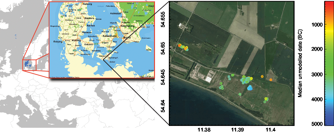
The wood and charcoal samples derive from 21 excavation fields within the 300-ha study area on the south coast of the island of Lolland (Figure 1). The wood samples are from stationary fishing devices (fish weirs) and artifacts such as ax handles, spears, bows, arrows, leisters, paddles, and boats, all of which had been lost or were ritually deposited in the shallow water of the former lagoons. The charcoal samples are from fireplaces (especially the oldest samples) or from cooking pits (especially the youngest samples). The samples were chosen for radiocarbon dating based on their archaeological significance, and not targeted at a pure δ13C study.

Figure 1 Map of the study area (left side, from www.krak.dk) and sample locations and radiocarbon dates of wooden artifacts plotted on an aerial photo of the site (right side), made with OxCal 4.3 and the calibration curve IntCal13 (Bronk Ramsey Reference Bronk Ramsey2009; Reimer et al. Reference Reimer, Bard, Bayliss, Beck, Blackwell, Bronk Ramsey, Buck, Cheng, Edwards, Friedrich, Grootes, Guilderson, Haflidason, Hajdas, Hatté, Heaton, Hoffmann, Hogg, Hughen, Kaiser, Kromer, Manning, Niu, Reimer, Richards, Scott, Southon, Staff, Turney and van der Plicht2013).
Wood and charcoal samples were species-identified by specialists from Moesgård Museum, Højbjerg, Denmark and the National Museum, Copenhagen, Denmark, by microscopic examination of fresh cuts through the samples. The samples were pretreated with a standard ABA treatment: 1M HCl for 1 hr, 1M NaOH for 3 hr (with renewed NaOH if necessary to remove all humics), both at 80°C, and finally 1M HCl overnight at room temperature to remove any CO2 absorbed during the NaOH treatment. Samples were oven-dried at 80°C, ca. 2 mg weighed out into pre-cleaned quartz tubes containing approximately 200 mg of CuO, evacuated and flame-sealed. Samples were combusted by heating those tubes to 900°C for 3 hr. The resulting CO2 was isolated cryogenically and reduced to pure carbon (graphite) with the H2 graphitization method, using Fe as catalyst and MgClO4 to absorb the water forming in the reaction (Vogel et al. Reference Vogel, Southon, Nelson and Brown1984; Santos et al. Reference Santos, Southon, Griffin, Beaupre and Druffel2007). The samples were radiocarbon dated using the HVE 1MV tandetron accelerator AMS system at the Aarhus AMS Centre (Olsen et al. Reference Olsen, Tikhomirov, Grosen, Heinemeier and Klein2016). Radiocarbon dates are reported as uncalibrated radiocarbon ages BP normalized to −25‰ according to international convention using online 13C/12C ratios (Stuiver and Polach Reference Stuiver and Polach1977). For the figures, we chose to use uncalibrated dates for practical reasons. Our conclusions would not be different if we had used calibrated dates. However, plotting the dates is much easier for radiocarbon dates with a mean and a standard deviation, instead of calibrated dates, where e.g. a probability distribution with two peaks would be represented misleadingly by only the main or median value and standard deviation.
δ13C was measured on sub-samples weighing ca. 0.25 mg using a continuous-flow IsoPrime IRMS coupled to an Elementar PyroCube elemental analyzer at the Aarhus AMS Centre. An in-house gelatine standard “Gel-A” was used as primary standard yielding ±0.2‰ for carbon analysis. Secondary in-house and international standards were used to check the normalization to the VPDB scale.
All statistical analysis was performed using MatLab, version R2018b. The errors on the linear fit in Figure 4C and D are estimated using a Bootstrap method with 5000 iterations. Figure 3 and Supplementary Figure 2 are computed using the BoxPlot function. The average values in Figure 2 are calculated using a moving window with a size of 100 or 250 14C years, which is stepped by 25 14C years in the interval from 2000 to 7000 14C years. A minimum of 5 data points is required for an average value to be computed. The error on the running mean value is estimated using the standard deviation divided by the square root of the number of data points.

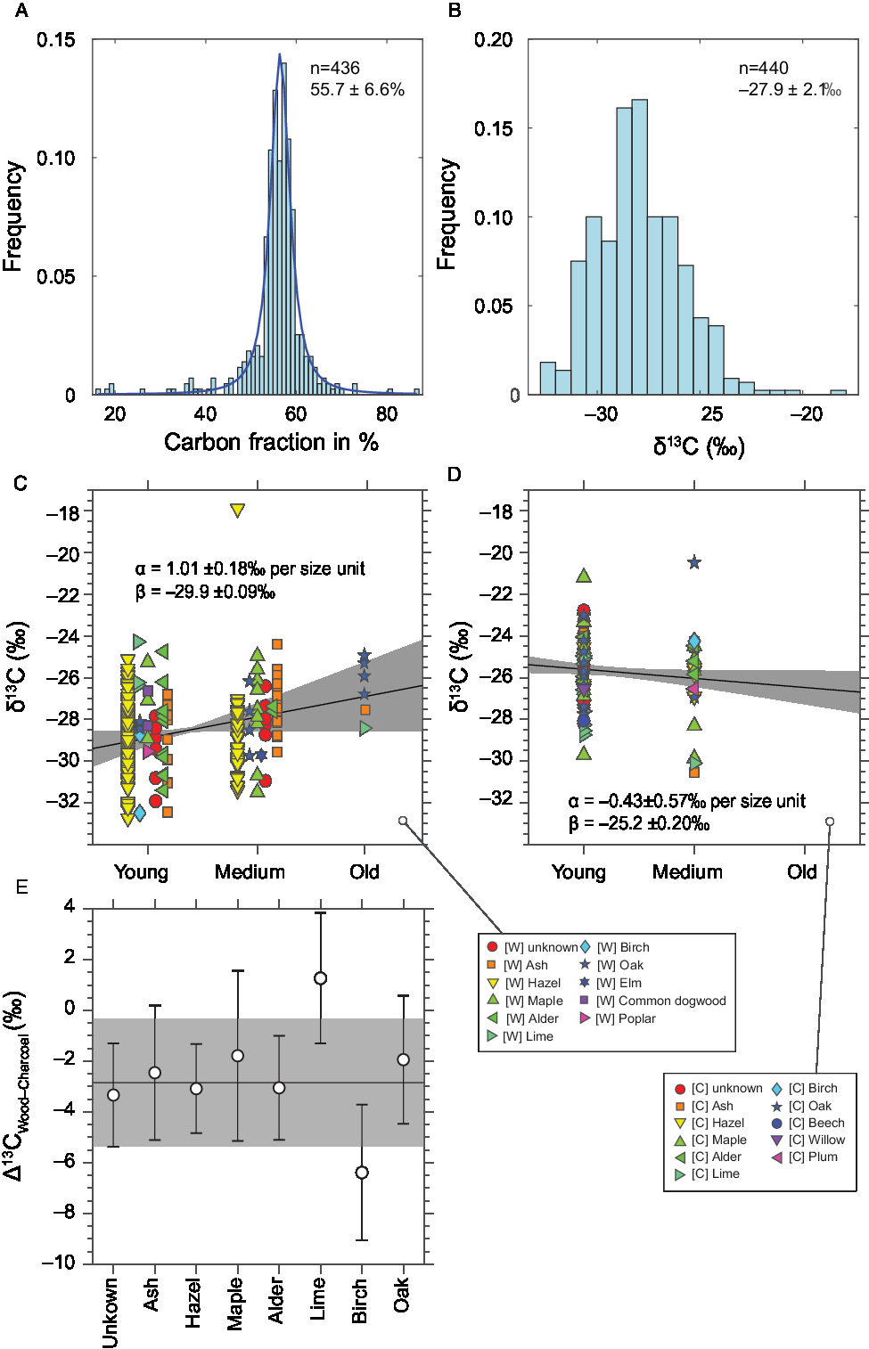
Figure 4 Histograms of A) the carbon fraction and B) the δ13C values of all samples, C) δ13C values of the wood and D) of the charcoal species arranged by age of the twig/branch/trunk; E) average δ13C difference between charcoal and wood per species (the line and shaded area show the average and standard deviation of all samples).
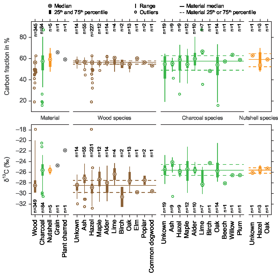
Figure 3 Box plots of the carbon fraction and δ13C values of the wood and charcoal samples of this study, also per species.
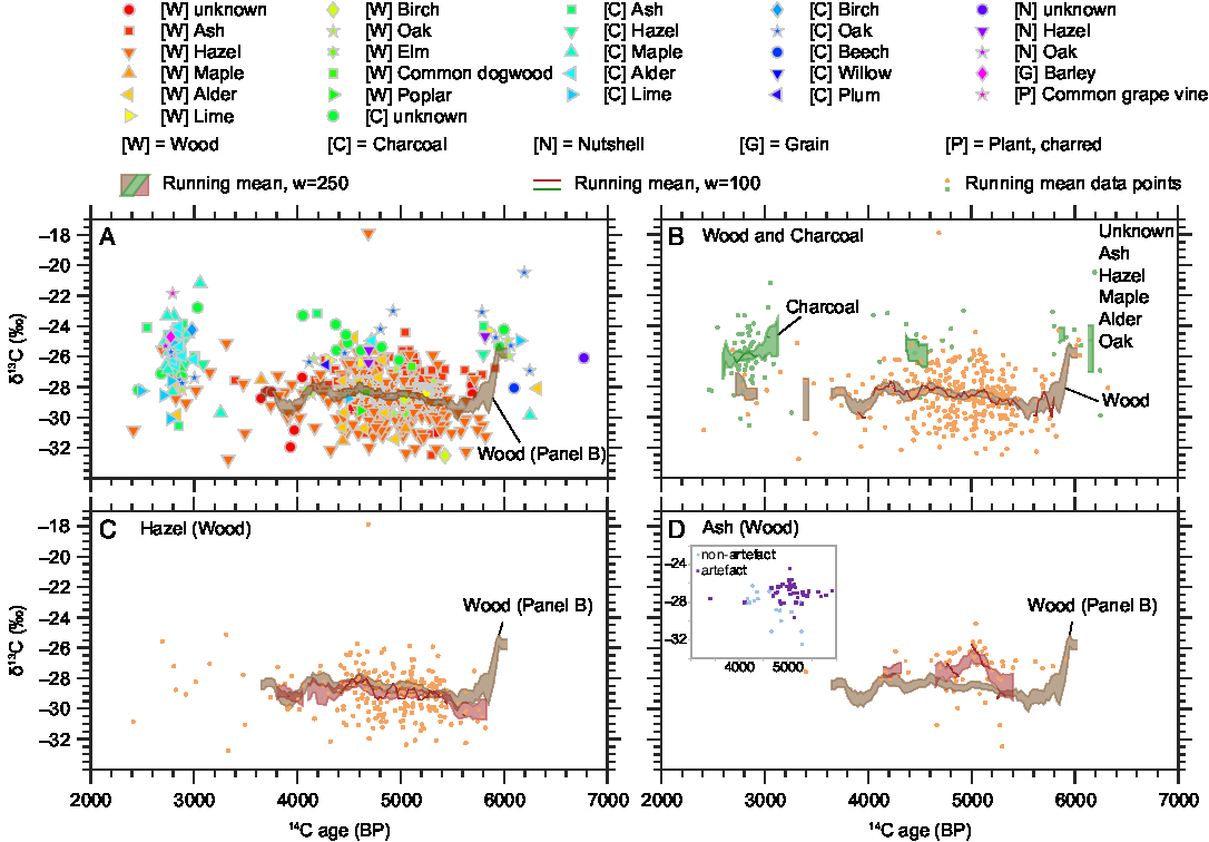
Figure 2 14C ages (BP) and δ13C values (‰ VPDB) of wood and charcoal samples from the study area with running means of the charcoal and wood data. Panel A shows all data, panel B differentiates between charcoal and wood, panels C and D show the wood δ13C values of the two most numerous species with their running means (red) on the background of the running mean of all wood samples (brown). An insert within panel D displays the ash wood δ13C values of artifacts (such as spears) versus non-artifacts (such as branches used in fish-weirs).
RESULTS
The whole range of δ13C values and radiocarbon ages is displayed in Figure 2. In Table 1, Figure 3 and Figure 4, the results are shown by species and material. Further information is displayed in two online supplementary figures—the δ13C values in relation to 14C age and carbon fraction for individual species in Supplementary Figure 1, and a comparison of carbon fraction and δ13C value of samples from artifacts (i.e., tools such as ax handles, spears, leister prongs, bows and arrows and boats that could have been brought to the site from farther away) versus samples such as firewood or branches for fish weirs, that would have been collected and used locally. As the measured 14C ages did not disagree with the ages expected on the background of the archaeological and stratigraphic information available, we consider the risk of post-depositional contamination affecting the 14C/12C and 13C/12C ratios to be minimal.
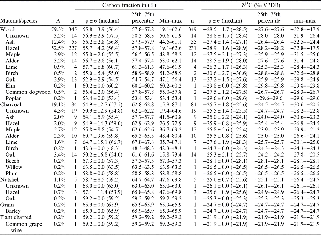
Table 1 Carbon fraction and δ13C values (range, average, median and standard deviation) for 440 wood and charcoal samples of this study. δ13C-14C scatter plots and δ13C-histograms of the most abundant species and of unidentified samples are displayed in Supplementary Figure 1, the δ13C averages and standard deviations (box plots) of all species are shown in Figure 3.

Figure 3 shows carbon fraction and δ13C value by material and species. Figure 4 is composed of several plots: Panels A and B are histograms of carbon fraction and δ13C values of all samples. Panels C and D show δ13C values of the individual samples grouped by the age of the branch/tree when it was cut, where “young” refers to small twigs with 2–7 year rings, “medium” to all bigger branches or artifacts made thereof, and “old” to tree stumps or trunks or artifacts made from those. Panel E shows the difference between wood and charcoal by species.
Figure 2 shows that the δ13C values span a range of more than 11‰, when one outlier of −17.9‰ is excluded. Not all periods are equally represented, for example, there is a relative lack of data from the period 4000–3000 BP. The bulk of data between 5500 and 4500 BP derives from excavations of waterlogged sites, many of them from fish weirs and settlement refuse that was deposited in shallow water. Therefore, many wood samples are preserved from this period. Another cluster of data from 3000 to 2500 BP originates from dryland excavations where only charcoal, and not wood, was well preserved. This period is therefore dominated by charcoal samples. This could explain the slightly higher δ13C values of the younger period. The running mean of all wood samples shows a decrease of ca. 2‰ just after 6000 BP and only small fluctuations thereafter (Figure 2). The running mean of the hazel δ13C values increases slightly between 5500 and 4500 BP, while the ash δ13C values peak around 5000 BP.
Table 1, Figure 3, and Figure 4E show that our charcoal samples tend to be more enriched in δ13C than wood. This could be caused by the preferential loss of the lighter carbon isotope (12C) during combustion of the volatile components of wood. The differences between wood and charcoal for the different species are summarized in Supplementary Table 1.
Wide ranges of δ13C values can also be observed within one species (Table 1, Figure 3, Supplementary Figure 1). Calculating the averages of the wood and charcoal samples of the different species shows that there can be up to 2–3‰ differences between species (Table 1). For example, the species with the highest average δ13C value is lime, with −26.3 ± 1.7‰ (n = 4), and the lowest is birch with −30.6 ± 2.7‰ (n = 2). Furthermore, Table 1, Figure 4E and Supplementary Figure 1 demonstrate again that in most cases, the charcoal is enriched in 13C.
DISCUSSION
Wood consists of a variety of different chemical compounds, produced by different biochemical pathways. One could therefore hypothesize that part of the variability of the measured δ13C values on wood are caused by the differential preservation of the different compounds, and that focusing on cellulose would reduce the variability. However, plant remains are reported to retain the original δ13C signal after millennia (Metcalfe and Mead Reference Metcalfe and Mead2019). Furthermore, there is very little evidence that the variability in cellulose would be smaller, not even for individual trees of the same species growing under very similar conditions (McCarroll and Loader Reference McCarroll and Loader2004). δ13C variations have also been found within the cellulose of one single tree ring, e.g. seasonal variation of 1–2‰ between earlywood and latewood, or variation of 1–4‰ around the circumference of a tree ring (Francey and Farquhar Reference Francey and Farquhar1982). Both charred and uncharred plant parts are reported to retain the original δ13C signal, especially when an acid-base-acid pretreatment precedes the measurements (DeNiro and Hastorf Reference DeNiro and Hastorf1985). Further, we observe no correlations between the δ13C values and carbon content (%C) for any of the identified species (Supplementary Figure 1). Therefore, we are confident that the variability in our wood samples reflects the variability of the δ13C values of the original wood.
In most species, the charcoal has less negative δ13C values than the wood. This implies that either the most labile components of the wood are depleted in 13C, or that generally the 13C-depleted molecules are most easily lost during charring. As we find this δ13C-enrichment due to charring fairly consistently for different species and throughout time, this could indicate a general mechanism—in contrast to the literature, where both enrichment, depletion and unchanged δ13C values are reported (see the Introduction and e.g. Ascough et al. Reference Ascough, Bird, Wormald, Snape and Apperley2008 for an overview). The nutshells of both species, hazel and oak, have intermediate δ13C values between wood and charcoal (see Supplementary Figure 1).
One could expect that with such a large dataset, effects such as a climatic influence on the δ13C values could be observed. Commonly δ13C analysis of the cellulose fraction of tree rings is used for climate reconstruction (e.g. McCarroll and Loader Reference McCarroll and Loader2004). However, significant correlations between the bulk wood and cellulose δ13C values indicate the bulk wood values would be a good proxy for cellulose values, and they have both been found to correlate significantly with summer temperature and growing season precipitation (Hemming et al. Reference Hemming, Switsur, Waterhouse, Heaton and Carter1998; Verheyden et al. Reference Verheyden, Roggeman, Bouillon, Elskens, Beeckman and Koedam2005; Taylor et al. Reference Taylor, Brooks, Lachenbruch, Morrell and Voelker2008; Mischel et al. Reference Mischel, Esper, Keppler, Greule and Werner2015). Thus, one could speculate whether data like those presented in this study could be used for climate reconstruction as well. However, this would certainly require better temporal resolution, as we were not able to find any trends with time in our dataset (Figure 2). Furthermore, any long-term climatic trends could be hidden in the large δ13C variation of the data. Charcoal δ13C values were also proposed as a climate proxy (Ferrio et al. Reference Ferrio, Alonso, López-Melción, Araus and Voltas2006). However, even though they are correlated to wood δ13C values and were a useful proxy for aridity in the cited study, we do not expect that trees in Denmark have been water-limited at any time in prehistory, and we have not found a long-term δ13C trend in our charcoal or wood samples. However, climate reconstruction could be possible with tree-ring measurements of Danish trees, because correlations of δ13C with ring width, temperature and precipitation have been found in Dutch trees, in a climate similar to the Danish climate (Francey and Farquhar Reference Francey and Farquhar1982).
The time trends mentioned above in the Results section (see also Figure 2) cannot be explained by environmental or climatic factors alone, as we observe different trends for the two most dominant species, hazel and ash (Figure 2, panels C and D). The running mean of the hazel δ13C values increases slightly between 5500 BP and 4500 BP, but no similar trend can be found in the other species, and we do not yet have an explanation for it. The δ13C value of the ash sample peaks around 5000 BP, in contrast to the δ13C values of other species (Figure 2 and Supplementary Figure 1). An explanation for this phenomenon might be found in the δ13C differences between artifacts (spears and paddles) and non-artifacts (branches used in fish weirs)—the δ13C values for artifacts are higher than those for non-artifacts (Supplementary Figure 2 and insert in Figure 2, panel D). In the time around 5000 BP, there was a peak in the ritual deposition of artifacts in shallow coastal water, including spears and paddles made of ash. Those were made of stems or older branches of ash, while the ash wood used for fish weirs was much younger, thus carrying a possible juvenile effect that could lower the δ13C values. Furthermore, spears and paddles could have been produced elsewhere and been transported to the study region, carrying another region’s isotope signature, while branches for fish weirs were most probably collected locally. Lev-Yadun et al. (Reference Lev-Yadun, Lucas and Weinstein-Evron2010) found, for a different environment, that imported wood could cause apparent δ13C variations. The overall running mean of the wood δ13C values decreases by about 2‰ after 6000 BP. This is probably caused by the different species analyzed here: the dataset before 6000 BP is dominated by oak and lime, which have comparatively high δ13C values (Figure 3). After 6000 BP, hazel dominates the dataset and lowers the average wood δ13C values as its δ13C values are lower than those of oak and lime (Figure 3). This could indicate a changing environment due to the rising sea level, where an oak-dominated inland forest was replaced by a more open, hazel-dominated coastal woodland. However, the most probable explanation is the changing resource use by the prehistoric people: as the area turned into a coastal landscape, they started to build stationary fishing devices, primarily from hazel branches. Finally, the 2‰ drop after 6000 BP could also be a result of the small number of samples from this period. Ideally, more wood samples from around 6000 BP should be analyzed, also including hazel samples.
Although all samples come from an area that is ca. 2.5 km across at its maximum, the range of measured δ13C values is as broad as that of other studies analysing samples from all over the world (e.g. Poole and Bergen Reference Poole and Bergen2006). Also, within one species, the range of δ13C values was almost as large as that of our entire dataset. The same effect was observed by Van de Water et al. (Reference Van de Water, Leavitt and Betancourt2002), who found that individuals growing at the same site had the same degree of variability as plants along the entire altitudinal gradient. This could be due to the micro-environment in which the trunks and branches grew. For example, wood δ13C values were observed to vary with sampling height within one individual tree, and whether the tree was shaded or exposed to sunlight (Wickman Reference Wickman1952; Li and Zhu Reference Li and Zhu2011; McDowell et al. Reference McDowell, Bond, Dickman, Ryan, Whitehead, Meinzer, Lachenbruch and Dawson2011). In dense forests, the CO2 is 13C-depleted compared to atmospheric CO2. This mechanism is known as the canopy effect and has been observed both in trees and in herbivores, where tree samples from lower heights in dense forests and herbivore populations from dense forests have more depleted δ13C values than those from open sites (Vogel Reference Vogel1978; Medina and Minchin Reference Medina and Minchin1980; van der Merwe and Medina Reference van der Merwe and Medina1991; Noe-Nygård and Hede Reference Noe-Nygård and Hede2006; Drucker et al. Reference Drucker, Bridault, Hobson, Szuma and Bocherens2008). Also, a juvenile effect, as explained in the introduction, could influence our δ13C values. Therefore, we divided our samples into age groups and found that the youngest branches tend to have lower δ13C values (Figure 3C). However, we were not able to distinguish young trees from young branches on old trees, which might explain the broad range of δ13C values for the youngest group.
Our study site would have been ideal to show whether environmental changes have an effect on the δ13C values of wood, because the rising sea level caused large changes in the gently sloping terrain. In spite of the substantial environmental changes at the study site, however, there are almost no temporal trends in our δ13C data. The exception is a 2‰ increase in the average δ13C values of wood samples from 6000 to 4200 BP. This corresponds to the period of strong relative sea level rise, as shown in Philippsen (Reference Philippsen2018: Fig. 4). One hypothesis to explain the increasing δ13C could be the transition from a dense inland forest to a more open coastal forest, possible further opened up by human activity. Ongoing archaeological and palaeo-ecological research could answer this question in the future. Short-term fluctuations might be present in long series of individual tree rings, but we did not have the possibility to analyze them. This study could be improved further if samples from the same species had been available for the entire time range, or if all species had been represented by the same number as the dominating hazel.
Although there are differences in the average δ13C values of the different species, their δ13C ranges overlap to a large degree (Figures 3 and 4, Supplementary Figure 1). Therefore, the results of this study cannot be used to examine details in photosynthesis and plant physiology between different species. This would only be possible if there were significant differences between the species. Similar results have been observed in different cereal species, usually between 1‰ and 5‰ for one site (Hammers in prep., Fiorentino et al. Reference Fiorentino, Caracuta, Casiello, Longobardi and Sacco2012; Lightfoot and Stevens Reference Lightfoot and Stevens2012; Bogaard et al. Reference Bogaard, Fraser, Heaton, Wallace, Vaiglova, Charles, Jones, Evershed, Styring, Andersen, Arbogast, Bartosiewicz, Gardeisen, Kanstrup, Maier, Marinova, Ninov, Schäfer and Stephan2013; Kanstrup et al. Reference Kanstrup, Holst, Jensen, Thomsen and Christensen2014; Styring et al. Reference Styring, Ater, Hmimsa, Fraser, Miller, Neef, Pearson and Bogaard2016, Reference Styring, Charles, Fantone, Hald, McMahon, Meadow, Nicholls, Patel, Pitre, Smith, Soltysiak, Stein, Weber, Weiss and Bogaard2017; Gron et al. Reference Gron, Gröcke, Larsson, Sørensen, Larsson, Rowley-Conwy and Church2017; Brinkkemper et al. Reference Brinkkemper, Braadbaart, van Os, van Hoesel, van Brussel and Fernandes2018), although the ranges of those plants were not as broad as those in this study. This difference between our study and those cited above is remarkable, as one would expect a greater variability in a plant that is subjected to different cultivation and management practices, in addition to the natural variation that might be found in unmanaged plants.
The δ13C values of plants are relevant for palaeodietary studies. On the one hand, plants were directly consumed by humans—not wood of course, but leaves, fruits, roots and tubers from plants. The broad δ13C ranges of trees that were encountered in this study thus serve as a cautionary tale for establishing useful plant baseline isotopic values for palaeodietary reconstruction. The δ13C values of edible plant parts could vary as much as those of our wood and charcoal samples. Furthermore, the foliage of the trees analyzed here could have served as fodder both for hunted animals as well as for domesticated animals. Although most of the variation found in the trees would have been averaged out in the transformation from plant to animal tissue (the average δ13C value of a herbivore’s total diet reflects the average of the plant δ13C values of all plants consumed), it should be kept in mind that some of the variability might be transferred up the food chain. However, we cannot make direct comparisons between wood and foliage δ13C values, as there can be considerable fractionation between wood and leaves. For example, Li and Zhu (Reference Li and Zhu2011) found that the leaves were enriched in δ13C in comparison to the trunk and branches. In any case, isotope values of modern and archaeological tree samples are not directly comparable due to the δ13C Suess effect (Suess Reference Suess1955; Revelle and Suess Reference Revelle and Suess1957), but the general fractionation trends will still be approximately the same. Therefore, although there might be deviations in the absolute values, we suggest that baseline data are collected for a broad range of plants for future palaeodietary studies.
CONCLUSION
In this study, we measured 14C ages and δ13C values on a total of 440 archaeological wood, charcoal and nutshell samples. We found that their δ13C values span a range of more than 11‰. Also, within one single species, ranges of ca. 10‰ were observed. There is some variation in δ13C values between different species, but the ranges overlap considerably (e.g., Table 1 and Figure 3). A general time-dependence of the δ13C values was not observed for the study period (Figure 2). The results presented here show that large variations can be expected at the base of the food chain, which can add uncertainty to palaeodietary reconstructions. In the future, we will try to link the δ13C values to the small-scale environment of where the tree grew—e.g., in a dense forest, one would expect lower δ13C values than in an open woodland.
ACKNOWLEDGMENTS
We would like to thank all the archaeologists and technical staff from Museum Lolland-Falster for their support in the field and storage facilities, for their constant helpfulness and interest in scientific archaeology.
SUPPLEMENTARY MATERIAL
To view supplementary material for this article, please visit https://doi.org/10.1017/RDC.2019.138