INTRODUCTION
Grain-size distributions (GSDs) are one of the most widely used proxies in paleoenvironmental and paleoclimatological investigations of sedimentary deposits, as they provide information on sediment source, depositional processes, and the sedimentary environment (Visher, Reference Visher1969; Ghosh and Mazumder, Reference Ghosh and Mazumder1981; Qiang et al., Reference Qiang, Chen, Zhou, Xiao, Zhang and Zhang2007; He et al., Reference He, Zhao, Song, Liu, Chen, Zhang and Liu2015). Statistical parameters such as the mean, median, standard, deviation, kurtosis, and skewness have been used to characterize GSDs and to infer variations in hydrodynamic conditions, eolian activity, and sediment source (Inman, Reference Inman1952; Blott and Pye, Reference Blott and Pye2001; Fournier et al., Reference Fournier, Gallon and Paris2014). In addition to these summary statistics, approaches to the decomposition of grain-size frequency distributions into components include graphic methods (e.g., CM patterns, where C the one percentile and M the median diameter) (Passega, Reference Passega1964), analytic methods (Court, Reference Court1949; Clark, Reference Clark1976), and numerical methods (Clark, Reference Clark1976). A more recent analytic approach is the standard deviation method, which is used for classifying the GSD to determine the most environmentally sensitive components (Boulay et al., Reference Boulay, Colin, Trentesaux, Pluquet, Bertaux, Blamart, Buehring and Wang2003). However, these approaches are generally based on the analysis of one percentile-median diameter part of, rather than the entire, GSD.
Several methods have been developed for mathematical unmixing of complete GSDs, such as curve fitting (Sun et al., Reference Sun, Bloemendal, Rea, Vandenberghe, Jiang, An and Ruixia2002; Paterson and Heslop, Reference Paterson and Heslop2015), eigenspace analysis (Weltje, Reference Weltje1997; Weltje and Prins, Reference Weltje and Prins2003; Dietze et al., Reference Dietze, Hartmann, Diekmann, Ijmker, Lehmkuhl, Opitz, Stauch, Wünnemann and Borchers2012), and a recently developed Bayesian method (Yu et al., Reference Yu, Colman and Li2015). These methods have proved effective in extracting information on provenance, transport processes, and the depositional environment of sediments; however, all of these methods have deficiencies. As discussed by Weltje and Prins (Reference Weltje and Prins2007), the curve-fitting method is based solely on the fitting of a series of empirical curves to the GSD and ignores their geologic context. Eigenspace analysis may produce uneven spectra because of the transformation and communality of grain-size compositional data, which makes interpretation difficult and confusing (Yu et al., Reference Yu, Colman and Li2015). The Bayesian method, because of the large number of iterations needed, may require a large amount of computation time if the data set is very large; furthermore, low-probability distributions may be ignored even though they may potentially be important.
Cluster analysis is a genetic type of multivariate statistical analysis and has been widely applied in statistics, mathematics, computer science, economics, and biology. Cluster analysis applied to sedimentary grain-size data is usually used for stratigraphic subdivision or to determine the sources of sediments (Donato et al., Reference Donato, Reinhardt, Boyce, Pilarczyk and Jupp2009; Grimm et al., Reference Grimm, Donovan and Brown2011; Liu et al., Reference Liu, Rühland, Chen, Xu, Chen, Chen, Huang, Xu, Chen and Smol2017). However, most of the studies have only employed the method to group a limited number of GSD parameters, such as the mean and standard deviation, and few studies have taken advantage of the entire distribution (Zhou et al., Reference Zhou, Chen and Lou1991; Nelson et al., Reference Nelson, Bellugi and Dietrich2014; Ordóñez et al., Reference Ordóñez, Ruiz-Barzola and Sierra2016). In addition, because of the problems of determining cluster number and cluster centers, no prior study has used cluster analysis for endmember modeling. Here we propose a new endmember model for unmixing GSDs based on hierarchical clustering endmember modeling analysis (CEMMA). Within our new model, the number of endmembers is inferred based on changes in agglomeration coefficients, and the spectra of endmembers are determined from the average distance between the samples in the clusters. Our proposed method thus provides a new way to objectively determine the number and spectrum of GSD endmembers that contribute to sediment, allowing us to unmix varying GSDs in time.
OVERVIEW OF ENDMEMBER MODELING ANALYSIS
Endmember modeling of GSDs was first proposed by Weltje (Reference Weltje1997), who showed that the compositional variation among a series of GSDs can be regarded as the result of the physical mixing of a fixed number of endmembers. This relationship can be expressed as a linear mixing model:
 $$X\,{\rm {\equals}\,}M{\rm \,{\asterisk}\,}B{\rm \,{\plus}\,}E.$$
In this model, matrix X(n×p) is the GSD data set in which each row represents one observed GSD with p different sizes that sum to 100%. Matrix M(n×q) represents the proportional contributions of endmembers to each observation; B(q×p) is a matrix containing q endmembers, each of which is a vector consisting of p elements; and E(n×p) represents the errors of the model. In order to accurately apply this model, three issues must be addressed: the number of endmembers, the spectra of the endmembers, and the fractions of the endmembers in each sample (Renner, Reference Renner1991). These problems can be addressed by using endmember model analysis based on hierarchical clustering (HC), described subsequently.
HIERARCHICAL CLUSTERING ENDMEMBER MODELING ALGORITHM
The sediments accumulating within lake basins have a range of provenances and are transported by various mechanisms. Sediment accumulation integrates these sources and processes, such that the GSD of a given sediment sample represents a mixture of sediments that correspond to different provenances and/or transport mechanisms. However, it can be assumed that given a sufficiently long time series of GSDs, there will be relatively brief intervals in which sediment provenance and transport are sufficiently stable to produce uniform GSDs that will represent those specific conditions. Therefore, what is required is a method of determining GSDs that represent those intervals.
The hierarchical clustering algorithm
The HC algorithm organizes data into a hierarchical structure according to a proximity matrix. HC attempts to construct a treelike nested structure that partitions original data and builds a hierarchy of clusters (Xu and Wunsch, Reference Xu and Wunsch2005). Two major issues must be solved when using HC analysis. The first is the similarity measure that can be used as a scalar distance between different clusters, and the second is the linkage method that orders the clusters to produce a unique and meaningful solution (Johnson, Reference Johnson1967; Gruvaeus and Wainer, Reference Gruvaeus and Wainer1972; Langfelder et al., Reference Langfelder, Zhang and Horvath2008). In this study, we used the average linkage as the linkage method between groups, which is defined on the basis that the similarity between two clusters is equal to the mean distance between elements of each cluster (http://home.deib.polimi.it/matteucc/Clustering/tutorial_html/hierarchical.html [accessed December 6, 2016]), and the city-block distance, which is less influenced by very large differences between just a few of the variables in high dimensional vectors (Kaufman and Rousseeuw, Reference Kaufman and Rousseeuw2009), is used to quantify the similarity between GSDs. The city-block distance between two GSDs ( x i , x j ) is expressed as follows:
 $$d_{{\left( {i,j} \right)}} {\equals}\mathop{\sum}\limits_{k{\equals}1}^p {\left| {x_{{ik}} \,{\minus}\,x_{{jk}} } \right|} ,$$
where d(i, j) is the distance between two GSDs x i and x j , p is the number of size classes in each GSD, and d(i, j) expresses the degree of difference between curves x i and x j . If observations x i and x j are highly similar, d(i, j) will be small, whereas dij is large if the distributions are highly dissimilar (Nelson et al., Reference Nelson, Bellugi and Dietrich2014).
The principal steps in calculating a hierarchical cluster, after Johnson (Reference Johnson1967), are as follows:
Step 1: Assign each GSD to be its own cluster, and calculate the distance d (i, j) between all pairs of clusters using the city-block distance (Eq. 2).
Step 2: Find the most similar pair of clusters in the initial clustering and merge them into a new single cluster, designated pair rs, as follows:
 $$d_{{\left( {rs} \right)}} \,{\equals}\,{\rm min}\,d_{{\left( {i,j} \right)}} ,$$
where d (rs) is the minimum d (i, j) of all distances of clusters.
Step 3: Compute the distance between the new cluster and the other clusters.
Step 4: Repeat steps 2 and 3 until all clusters are merged into a single cluster.
Estimating the number of clusters
A major challenge in cluster analysis is determining the optimal number of clusters. Many methods have been used, including the gap statistic (Tibshirani et al., Reference Tibshirani, Walther and Hastie2001), the dynamic tree cut method (Langfelder et al., Reference Langfelder, Zhang and Horvath2008), and the density peak (Rodriguez and Laio, Reference Rodriguez and Laio2014). However, all of these methods have inherent limitations, and few of them can be used efficiently in the analysis of GSDs.
In the “bottom-up” hierarchical cluster analysis used here, the agglomeration coefficient indicates the within-group variance of two clusters combined at each successive stage of the clustering and therefore provides a simple and objective means of determining the optimum stage for terminating the clustering and the total number of clusters (Everitt et al., Reference Everitt, Landau, Leese and Stahl2011). This is because a large change in the agglomeration coefficient between two stages of clustering indicates that heterogeneous clusters are being combined, and the result has a larger total variance. Thus, this approach can be used to judge whether an optimal cluster solution has been achieved (Hill et al., Reference Hill, Brennan and Wolman1998). A significant change in the agglomeration coefficient can be termed a “knee” (Salvador and Chan, Reference Salvador and Chan2004), which can be determined by calculating and graphing the change in agglomeration coefficients as a function of the stages in the cluster analysis (i.e., the total number of clusters). Large changes in the agglomeration coefficient as a function of the number of clusters will signify the merger of dissimilar clusters and therefore indicate the optimum number of clusters. As suggested by Salvador and Chan (Reference Salvador and Chan2004) and Chiu et al. (Reference Chiu, Fang, Chen, Wang and Jeris2001), there are two efficient ways to find the “knee” of a curve. One is to look for the largest magnitude difference between two adjacent points of the change in the agglomeration coefficient; the other is to calculate the jump in ratio change between two points. Here, we use the first method to find the “knee” because it involves little computation and easy operation.
Determining the unmixed grain-size distributions
The unmixed GSDs are defined as the most typical GSDs in the data set that are representative of their clusters—in other words, they have the maximum degree of similarity to every GSD within their cluster. This is calculated to be the GSD that produces the minimum average distance in the clusters:
 $$C_{{\left( q \right)}} \,{\equals}\,{\rm min}\,d_{{\left( {q,ks} \right)}} ,$$
where ks is a cluster in which all the GSDs can be assumed to have been generated by similar depositional processes, and q denotes the most representative GSDs, which have maximum similarity to every GSD in cluster ks.
Fractions of each endmember within a sample
In the linear mixing model, if the number of endmembers and their compositions can be determined accurately, the fraction of each endmember contributing to each sample can be estimated using standard least squares techniques (Weltje, Reference Weltje1997). For compositional data (i.e., GSDs), the fraction of each endmember in each sample should be nonnegative and sum to 1, so that the fraction of each endmember can be calculated by a nonnegative least squares algorithm and scaled to a constant sum (Weltje and Prins, Reference Weltje and Prins2007), as follows:
 $$\mathop{\sum}\limits_{k{\equals}1}^q {m_{{ik}} \,{\equals}\,1,} $$
where mik is the proportional contribution of the endmembers to each observation, and q is the number of the endmember. All of the mik values constitute the fractions matrix M(n×q) .
A CASE STUDY: THE SEDIMENTS OF WULUNGU LAKE, JUNGGAR BASIN, CHINA
A GSD data set from the sediments of Wulungu Lake in the Junggar Basin, China (Fig. 1), was used to test the CEMMA method. Wulungu Lake is a hydrologically closed terminal lake fed mainly by the Wulungu River. The sediments studied are from a 7-m-long core (WLG11E) taken from the central part of the lake (47°14.40′N, 87°13.10′E) in a water depth of 18 m. The sediments studied here accumulated during Marine Oxygen Isotope Stage 3, between ~25,300 and 51,600 cal yr BP (Zhang et al., Reference Zhang, Zhou, Zhang, Hao, Zhao and An2016). The core is mainly composed of silty clay with occasional thin intercalated layers of silt or gypsum. Five lithologic units can be defined on the basis of sediment color and composition, as follows (see Fig. 2): unit I (901–769 cm) is dominated by gray silty clay; unit II (769–613 cm) consists of yellowish silty clay (769–711 cm), gray silty clay (711–662 cm), and brown silty clay (662–613 cm); unit III (613–400 cm) consists of yellowish silty clay; unit IV (400–294 cm) consists of gray silty clay (400–371 cm and 349–294 cm) and yellowish silty clay with gypsum (371–349 cm); and unit V (294–193 cm) consists mainly of brown silty clay.
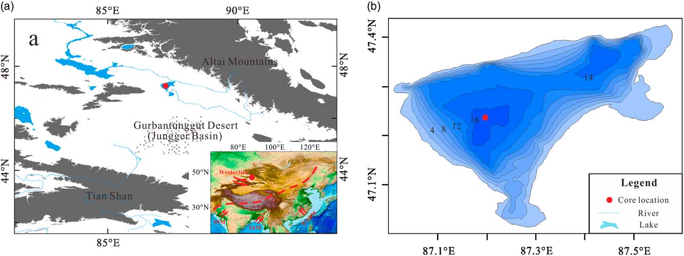
Figure 1 (a) Topography of the study area. The red dot indicates the location of Wulungu Lake. Gray-shaded areas are mountains (elevation >4374 m). Inset map shows the location of the study area within Asia, with trajectories of the major atmospheric circulation systems indicated by red arrows and the modern Asian summer monsoon limit indicated by the red dashed line (after Chen et al., Reference Chen, Yu, Yang, Ito, Wang, Madsen and Huang2008, Reference Chen, Chen, Holmes, Boomer, Austin, Gates, Wang, Brooks and Zhang2010). EASM, East Asian summer monsoon; ISM, Indian summer monsoon. (b) Bathymetry of Wulungu Lake (contours at 2 m intervals) with the location of core WLG11E indicated by the red dot (Wu et al., Reference Wu, Ma and Zeng2013). (For interpretation of the references to color in this figure legend, the reader is referred to the web version of this article.)
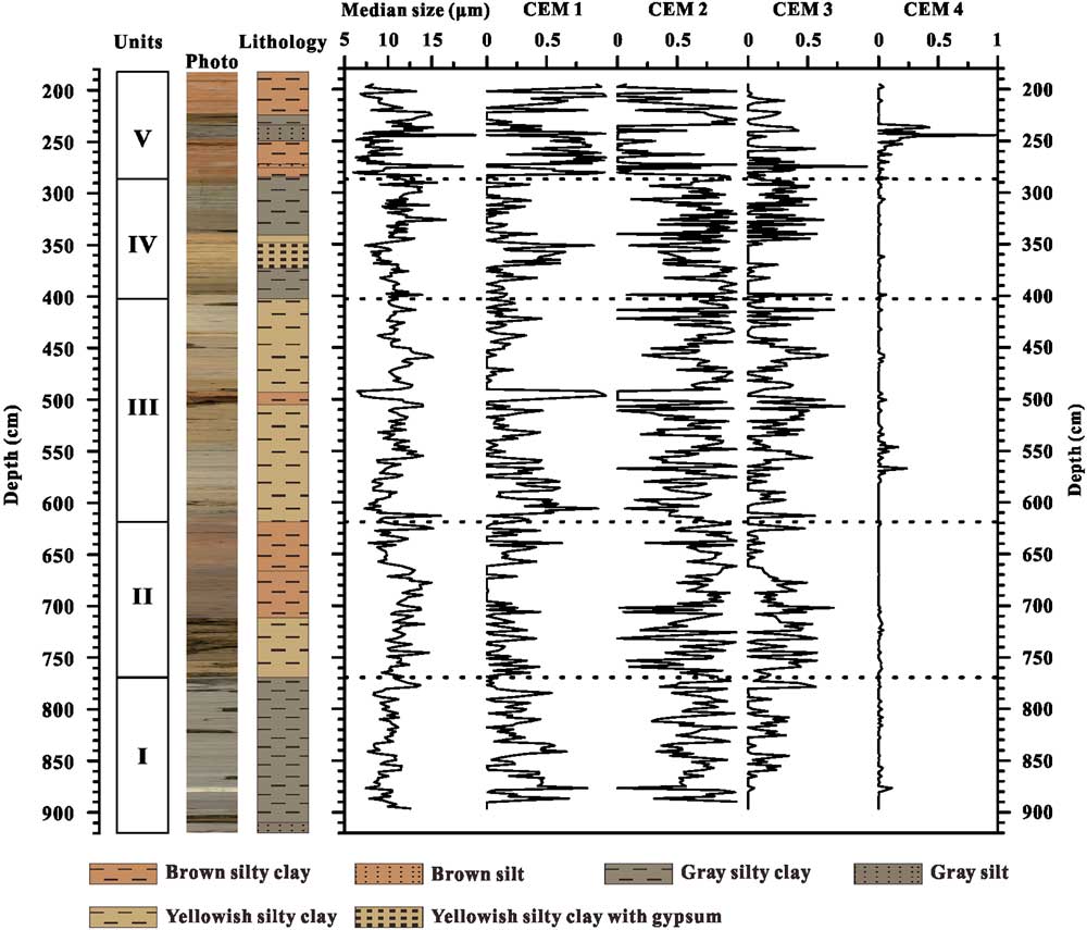
Figure 2 (color online) Lithologic units, graphic lithology, and changes in sediment median size and endmember fractions (clustering endmember [CEM] 1 to CEM 4) plotted against depth for core WLG11E.
A total of 373 samples were obtained at 2 to 3 cm intervals from the core for grain-size analysis. The samples were pretreated with 10% H2O2 to remove organic matter and 10% HCl to remove carbonates, rinsed with deionized water, and then dispersed with 10 mL of 0.05 mol/L (NaPO3)6 in an ultrasonic bath for 10 minutes. GSDs between 0.02 and 2000 μm were measured using a Malvern Mastersizer 2000 laser grain-size analyzer and assigned to 100 size classes. The GSDs are relatively uniform (Fig. 3a), with most samples possessing a modal grain size of around 11 μm (silt), whereas a few samples have additional peaks at around 40 μm (coarse silt) or between 300 and 800 μm (sand).

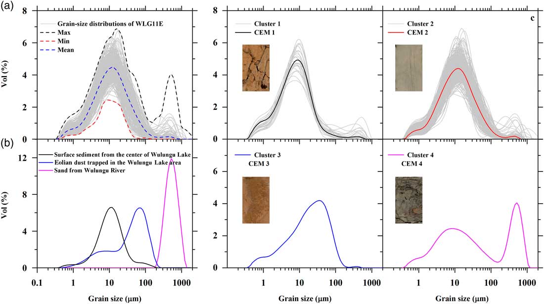
Figure 3 (a) Grain-size distributions (GSDs) of samples from sediment core WLG11E from Wulungu Lake (light-gray lines), including the maximum, minimum, and mean for each grain-size class. (b) GSD curves for surface sediment from the center of Wulungu Lake (black curve), eolian dust trapped near the ground surface in Wulungu Lake area (blue curve) (after Liu et al., Reference Liu, Herzschuh, Shen, Jiang and Xiao2008), and sand from the Wulungu River (magenta curve). (c) Results of clustering endmember modeling analysis for the sediments of core WLG11E from Wulungu Lake: four clustering endmember (CEM) unmixed GSDs (colored lines) and clusters (light-gray lines). Inset image shows the lithology of the relevant interval of the core. (For interpretation of the references to color in this figure legend, the reader is referred to the web version of this article.)
Applying the CEMMA method to the Wulungu Lake data, the agglomeration coefficients show a large change at four clusters (the red dot in Fig. 4), which thus defines the “knee” and indicates that the clustering should be terminated. Therefore, four optimal endmembers can be inferred from the CEMMA model in this example. The GSDs of the clustering endmembers (CEMs) are illustrated in Figure 3c. CEM 1 exhibits a unimodal peak with a dominant mode at around 8 μm (very fine silt and coarse clay), CEM 2 exhibits a symmetrical unimodal peak in the very fine silt range (mode at 13 μm), CEM 3 is characterized by an asymmetrical unimodal peak centered at around 40 μm (coarse silt), and CEM 4 exhibits a bimodal structure with a dominant mode at around 522 μm (sand) and a minor mode at around 8 μm (very fine silt and coarse clay). The GSDs of three modern sediment samples are also plotted (Fig. 3b). Surface sediments from the center of Wulungu Lake exhibit a unimodal distribution with a peak at around 10 μm, an eolian dust sample trapped in the Wulungu Lake area exhibits a slightly bimodal GSD with a dominant mode at around 58 μm and a minor mode at around 6 μm (Liu et al., Reference Liu, Herzschuh, Shen, Jiang and Xiao2008), and sand from Wulungu River exhibits an asymmetrical unimodal distribution with a peak at around 522 μm.
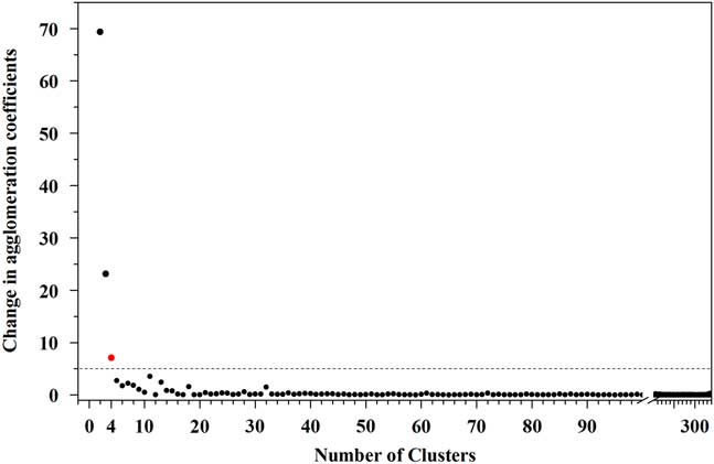
Figure 4 Change of the agglomeration coefficient versus number of clusters. The red dot is the “knee.” (For interpretation of the references to color in this figure legend, the reader is referred to the web version of this article.)
Changes in the fractions of endmembers versus depth are plotted in Figure 2. The first endmember (CEM 1) is dominant in brown silty clay, corresponding to lithologic unit V, and has an average fractional abundance of 0.47. CEM 2 exhibits high values in gray silty clay (units I and IV, with average values of 0.67 and 0.69, respectively). CEM 2 is also relatively high in yellowish silty clay (units II and III, with average values of 0.57 and 0.60, respectively). The third endmember (CEM 3) exhibits relatively low values down core (average of 0.15) and comparatively high values in yellowish silty clay (average of 0.21). CEM 4 is only recorded in a few layers with gray silt; it is represented in the interval from 247–234 cm, with an average value of 0.32.
DISCUSSION
In the CEMMA results (Fig. 3), CEM 1 and CEM 2 exhibit a similar GSD to surface sediments from the center of Wulungu Lake but have slightly different modal grain-size values of 8 and 13 μm, respectively. As indicated by the lithologies corresponding to these endmembers, CEM 1 is represented in brown silty clay and CEM 2 in gray silty clay. According to the results of a previous study (Zhang et al., Reference Zhang, Zhou, Zhang, Hao, Zhao and An2016), gray silty clay contains relatively high feldspar (17%) and low illite (35%), whereas brown silty clay has a high concentration of illite (47%) and a low concentration of feldspar (11%). Illite-rich sediments have been interpreted as representing relatively dry conditions (Singer, Reference Singer1984). Together with the lithology, it can be inferred that CEM 1 reflects the hydrodynamic energy of a very shallow lake environment, whereas CEM 2 reflects the hydrodynamic energy of a deep lake environment. Comparison of the GSDs of the CEM endmembers with those of modern samples (Fig. 3) indicates that CEM 3 exhibits a similar GSD to the eolian dust trapped in the Wulungu Lake area. Thus, this GSD indicates eolian transport of a local dust source via short-term suspension and saltation processes, probably by local storms in winter and spring when near-surface turbulent airflow prevails (Qin et al., Reference Qin, Cai and Liu2005; Qiang et al., Reference Qiang, Chen, Zhou, Xiao, Zhang and Zhang2007; Yu et al., Reference Yu, Colman and Li2015). CEM 4 has a similar distribution to a mixture of lacustrine suspended sediment and Wulungu River sediments and therefore can be interpreted as indicating the strength of the runoff into the lake.
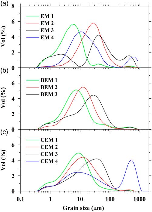
To estimate the performance of our CEMMA methods, we compare our CEMMA results with the corresponding endmembers obtained from the eigenvector rotation endmember modeling analysis (EMMA) (Dietze et al., Reference Dietze, Hartmann, Diekmann, Ijmker, Lehmkuhl, Opitz, Stauch, Wünnemann and Borchers2012) (Fig. 5a) and hierarchical Bayesian endmember modeling analysis (BEMMA) (Yu et al., Reference Yu, Colman and Li2015) (Fig. 5b). We calculate the modal size, sorting, skewness, and kurtosis of endmember spectra as suggested by Folk and Ward (Reference Folk and Ward1957) and also fit the endmember spectra to the WLG11E data set to calculate the error of reconstructed GSDs and the correlation coefficient between the reconstruction and original data (Table 1). The results show that the EMMA method gets the biggest error value (0.51) and poor reconstruction results (data set R 2 is 0.77). However, BEMMA and CEMMA results show similar values for the goodness-of-fit test; they both show lower error values (0.16) and higher correlation coefficient values (data set R 2 is 0.98). As to each endmember spectrum, the first endmember defined by all three methods is broadly similar, with a dominant mode at around 8 μm (Table 1). However, there are marked differences between the other three endmembers. First, as to the second endmember, the results for BEMMA (Bayesian endmember [BEM] 2) and CEMMA (CEM 2) exhibit a similar distribution with a symmetrical unimodal peak at around 13 μm. However, the EMMA result (endmember [EM] 2) is quite different, with a unimodal peak around 30 μm. With regard to the third endmember, the results for BEM 3 and CEM 3 exhibit a similar distribution with a modal peak at around 40 μm and with moderate sorting (1.94 and 1.84, respectively); however, EM 3 is poorly sorted (2.95) and exhibits a multimodal distribution with a fine peak around 3 μm and a coarse peak around 400 μm (Folk and Ward, Reference Folk and Ward1957). If the second and third endmembers are combined, the results for BEMMA and CEMMA are similar, but they differ from that of EMMA. This difference results from the absence of data for the fine and coarse size fractions, because in the EMMA method problems arise as a result of the transformation and communality of grain-size compositional data if the grain-size data have many zero components (Yu et al., Reference Yu, Colman and Li2015).

Figure 5 (color online) Comparison of endmember spectra for core WLG11E obtained using the eigenspace method (a), hierarchical Bayesian endmember modeling analysis (b), and hierarchical clustering endmember modeling analysis (this study) (c). BEM, Bayesian endmember; CEM, clustering endmember; EM, endmember.
Table 1 The parameters of endmember spectra and goodness-of-fit statistics for fitting the endmember spectra to the WLG11E data set using different endmember methods. BEM, Bayesian endmember; BEMMA, Bayesian endmember modeling analysis; CEM, clustering endmember; CEMMA, clustering endmember modeling analysis; EM, endmember; EMMA, endmember modeling analysis.

BEMMA does not calculate a fourth endmember. This is because the results of the Bayesian method can be influenced by the prior distributions and maximum likelihood of samples, with the consequence that information of low probability (frequency) may be ignored, even though it may potentially be of environmental significance (i.e., the fourth endmember).
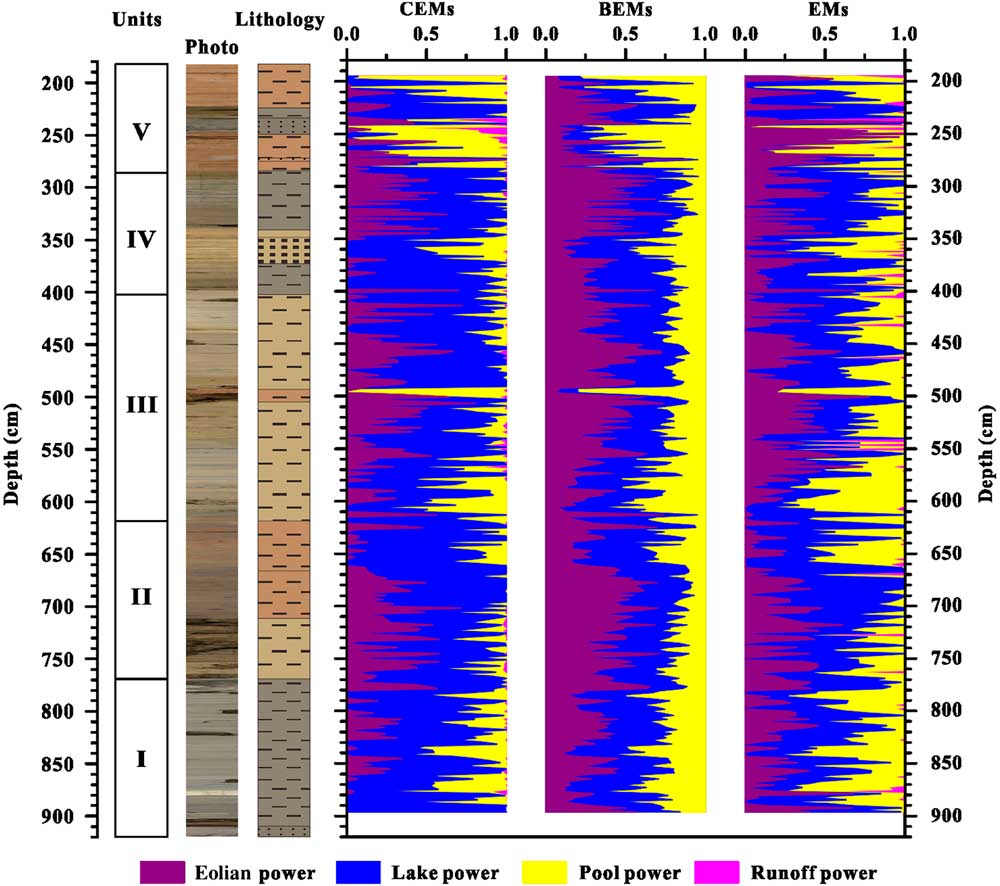
With regard to the fractions of each endmember produced by the different methods (Fig. 6), the results are generally in agreement with each other, and all of them coincide with the lithologic units. However, in contrast, because of the differences between the endmember spectra, “eolian energy” (the third endmember) exhibits slight differences between the three methods, and a value for “runoff energy” (the fourth endmember) is not provided by the BEMMA results. In summary, CEMMA endmembers show much better agreement with major lithologic units in our sediment core and major sedimentary processes operating in Wulungu Lake than do the other endmember modeling methods tested here.

Figure 6 (color online) Lithologic units, graphic lithology, and comparison of endmember fractions from hierarchical clustering endmember modeling analysis (clustering endmembers [CEMs], this study), hierarchical Bayesian endmember modeling analysis (Bayesian endmembers [BEMs]), and the eigenspace method (endmembers [EMs]).
In addition, our CEMMA method has several advantages over the EMMA and the improved BEMMA methods: (1) the computation time for large data sets is very low because the method does not use iterations; (2) CEMMA is not influenced by zero data values in the leading and trailing sides of compositional data; and (3) it takes advantage of lithologic information, which aids understanding of the depositional environments reflected by the endmembers.
Despite the overall effectiveness of the methodology presented here, the endmembers produced by our algorithm may not correspond exactly to the hydrodynamic and eolian processes that they reflect. In addition, the effectiveness of the method is restricted by the sampling resolution and the sediment accumulation rate. Finally, because of the fact that the fractions of the endmembers are nonnegative and always sum to 1, the endmember fractions do not correspond exactly to the strength of the corresponding environmental processes.
CONCLUSIONS
Endmember modeling analysis provides an effective means of unmixing GSDs in order to determine the provenance, transport mechanisms, and depositional environment of sediments. The fractions of endmembers can potentially be used as proxies for paleoenvironmental and paleoclimatic processes through different depositional environments. In this study, the CEMMA method, based on cluster analysis combined with least squares fitting is used to define GSD endmembers. The number of endmembers can be readily determined from the agglomeration coefficients, the endmember spectra are selected based on the average distance between samples within the clusters, and the fractions of each endmember are determined by a nonnegative least squares algorithm. In the lake sediment case study presented here, the interpretation of the endmembers uses variations in lithology to aid the assessment of sediment provenance. We conclude that the methodology provides an efficient means of identifying the most representative samples in very large data sets.
ACKNOWLEDGMENTS
We thank Dr. Jan Bloemendal for his thorough and constructive reviews that significantly improved the manuscript. This project was supported by National Key R&D Program of China (grant number. 2017YFA0603402), the National Natural Science Foundation of China (grant number. 41130102 and 41372180), and the Fundamental Research Funds for the Central Universities (grant number. lzujbky-2016-245).
Supplementary material
To view supplementary material for this article, please visit https://doi.org/10.1017/qua.2017.78