


1. Introduction
The technique of approximating a sub-Riemannian (degenerate) metric by Riemannian (non-degenerate) metrics was most likely first used by Korányi [Reference Korányi9] to study geodesics in the Heisenberg group. It was later used by Jerison and Sánchez-Calle [Reference Jerison and Sánchez-Calle8] to study subelliptic second order linear operators and by Monti [Reference Monti10] to study Carnot-Carathéodory metrics. These approximations are obtained by essentially adding a small multiple of the Euclidean metric and letting it go to zero. More structured approximations tailored to the nilpotent Lie algebra structure of the vectors fields generating the sub-Riemannian metric were introduced by Capogna and Citti and have become a powerful tool for studying nonlinear elliptic and parabolic partial differential equations in the subelliptic setting, see [Reference Capogna and Citti2, Reference Capogna, Citti, Donne and Ottazzi3, Reference Domokos and Manfredi6].
Of great interest is to determine what geometric and analytical properties are preserved by these approximations. Note, for example, that the Hausdorff dimension is certainly not preserved. Capogna, Citti and their collaborators [Reference Capogna and Citti2, Reference Capogna, Citti and Manfredini4, Reference Capogna, Citti and Rea5] have established that the constants in the volume doubling property and the Poincaré and Sobolev inequalities are stable under certain Riemannian approximations. Their proofs are based on the results of the seminal paper [Reference Nagel, Stein and Wainger11], and are valid for general systems of Hörmander vector fields.
The purpose of this note is to provide a direct and explicit proof of these facts in the case of Carnot groups, independent of the results of [Reference Nagel, Stein and Wainger11], which are not needed in the case of Carnot groups. We are motivated by the study of non-linear sub-elliptic equations in Carnot groups. We believe these simpler and constructive proofs might help us think of new ways to advance our understanding of the regularity of solutions to non-linear partial differential equations in Carnot groups.
Our proof makes very explicit the relation between the gradient of the approximating vector fields and the approximating distances (see remark 2.9 below) and gives an explicit expression of the constant in the Poincaré-Sobolev inequality in terms of the doubling constant [see formula (4.1) below].
The plan of the paper is as follows. In § 2, we set the notation, review properties of the various distances associated to the families of vector fields we use in our approximations, and prove the approximation property for these distances. In § 3, we provide our explicit proof of the doubling property and exhibit an explicit family of approximating gauges. And in § 4, we present Poincaré and Sobolev inequalities that hold uniformly for all the approximating metrics and where the relevant gradients approximate the Carnot group subelliptic gradient when the approximation parameter  $\varepsilon \to 0$.
2. Preliminaires
A Carnot group  $({{\mathbb {G}}}, \cdot )$ is a connected and simply connected Lie group whose Lie algebra
  $\mathfrak {g}$ admits a stratification
 \begin{equation} {{\mathfrak g}} = \bigoplus_{i=1}^{\nu} V^{i} , \end{equation}
where  $\nu \in {\mathbb {N}}$,
  $\nu \geq 2$ and
  $V^{i}$ is a vector subspace such that
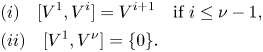 \begin{equation} \begin{aligned} & (i) \quad [V^{1}, V^{i}] = V^{i+1}\quad \text{if}\ i \leq \nu -1,\\ & (ii) \quad [V^{1}, V^{\nu}] = \{ 0 \}. \end{aligned} \end{equation}
Letting  $n_i =\dim (V^{i})$ and
  $n=n_1+\cdots +n_\nu$, it is always possible to identify
  $({{\mathbb {G}}}, \cdot )$ with a Carnot group whose underlying manifold is
  $\mathbb {R}^{n}$, and that satisfies the properties we describe next (see chapter 2 of the book [Reference Bonfiglioli, Lanconelli and Uguzzoni1]).
We write points  $x\in {{\mathbb {G}}}$ (identified with
  $\mathbb {R}^{n}$) as follows:
 \[ x=(x^{(1)}, \ldots, x^{(\nu)})=(x_{11}, \ldots, x_{1 n_1}, x_{21}, \ldots, x_{2n_2}, \ldots , x_{\nu 1}, \ldots , x_{\nu n_\nu}), \]
where  $x^{(i)}$ stands for the vector
  $(x_{i1}, \ldots , x_{i n_i})$ for all
  $i=1,\ldots ,\nu$. The identity of the group is
  $0\in \mathbb {R}^{n}$ and the inverse of
  $x\in \mathbb {R}^{n}$ is
  $x^{-1}=-x$.
The anisotropic dilations  $\{\delta _\lambda \}_{\lambda >0}$, defined as
 \[ \delta_\lambda(x)=(\lambda x^{(1)},\ldots,\lambda^{\nu} x^{(\nu)}) , \]
are group automorphisms. The number  $Q=\sum _{i=1}^{\nu } i n_i$ is the homogeneous dimension of the group, and it agrees with the Hausdorff dimension of the metric space
  $(G, d_0)$, where
  $d_0$ is defined below (definition 2.1). The Lebesgue measure is left and right invariant, and also
  $\delta _\lambda$-homogeneous of degree
  $Q$, that is
  $|\delta _\lambda (A)|=\lambda ^{Q}|A|$ for all
  $\lambda >0$ and measurable sets
  $A\subset \mathbb {G}$.
The Jacobian basis of  $\mathfrak {g}$ consists of left invariant vector fields
 \begin{equation} \{ X_{11}, \ldots, X_{1n_1},\ldots, X_{\nu 1}, \ldots, X_{\nu n_\nu}\} =\{X_{ij}\}^{i=1,\ldots,\nu}_{j=1,\ldots, n_i}, \end{equation}
which coincide with  $\{\partial _{x_{ij}}\}^{i=1,\ldots ,\nu }_{j=1,\ldots , n_i}$ at the origin
  $x=0$ and are adapted to the stratification; that is, for each
  $i = 1,\ldots ,\nu$ the collection
  $\{X_{i1},\ldots , X_{in_i}\}$ is a basis of the
  $i$-th layer
  $V^{i}$. As a consequence
  $X_{11},\ldots , X_{1n_1}$ are Lie generators of
  $\mathfrak {g}$, and will be referred to as horizontal vector fields.
The vector field  $X_{ij}$ is
  $\delta _\lambda$-homogeneous of degree
  $i$ and has the form
 \begin{equation} X_{ij}=\partial_{x_{ij}}+\sum_{k=i+1}^{\nu}\sum_{l=1}^{n_k} b_{ij}^{kl}(x^{(1)}, \ldots, x^{(k-i)})\partial_{x_{kl}}, \end{equation}
where  $b_{ij}^{kl}$ are polynomials
  $\delta _\lambda$-homogeneous of degree
  $k-i$, depending only on the variables
  $x^{(1)},\ldots , x^{(k-i)}$.
The exponential map Exp $: \mathfrak {g}\longrightarrow \mathbb {G}$ written with respect to this basis is the identity, i.e.,
 \begin{equation} \text{Exp}\left(\sum_{ij}x_{ij}X_{ij}\right)=x. \end{equation}
In the above formula we used the convention that the sum  $\sum _{ij}$ is extended to all indexes
  $i=1,\ldots , \nu$ and
  $j=1,\ldots ,n_i$, which we will use throughout this exposition. By a slight abuse of notation we also denote by
  $X_{ij}(x)$ the vector in
  $\mathbb {R}^{n}$ whose components are the components of the vector field
  $X_{ij}$ with respect to the frame
  $\{\partial _{x_{kl}}\}_{l=1,\ldots ,n_k}^{k=1,\ldots ,\nu }$ at the point
  $x\in \mathbb {R}^{n}$.
Definition 2.1 For  $x,y\in {{\mathbb {G}}}$ and
  $r>0$, let
  ${AC}_0 (x,y,r)$ denote the set of all absolutely continuous functions
  $\varphi \colon [0,1] \mapsto {{\mathbb {G}}}$ such that
  $\varphi (0) =x$,
  $\varphi (1) = y$ and
 \begin{equation} \varphi ' (t) = \sum_{j=1}^{n_1} a_{1j} (t)\, X_{1j} (\varphi (t))\quad\text{for a.e.}\ t \in [0,1] \end{equation}
for a vector of measurable functions  $a= (a_{11},\ldots , a_{1 n_1})\in L^{\infty }([0,1], \mathbb {R}^{n_1})$ with
 \begin{equation} \| a\|_{L^{\infty}([0,1], \mathbb{R}^{n_1})} = \mathrm{ess\,sup}\left\{|a(t)|= \left( \sum_{j=1}^{n_1} a^{2}_{1j}(t) \right)^{1/2} \colon t\in[0,1]\right\}< r. \end{equation}
Define the Carnot-Carathéodory distance as
 \[ d_0 (x,y) = \inf \{ r>0 \; | \; {AC}_0 (x,y,r) \neq \emptyset \} . \]
 Note that by the bracket generating property of  $\{X_{11}, \ldots , X_{1{n_1}}\}$ there is always an
  $r>0$ such that
  ${AC}_0 (x,y,r) \neq \emptyset$.
Proposition 2.2 For  $x,y\in {{\mathbb {G}}}$ and
  $1\le p\le \infty$ define the distance
  $d_p(x,y)$ as in definition 2.1 replacing
  $\| a\|_{L^{\infty }([0,1], \mathbb {R}^{n_1})}$ by
  $\| a\|_{L^{p}([0,1], \mathbb {R}^{n_1})}$. Then, we have
  $d_p(x,y)=d_0(x,y)$.
Proof. See proposition 3.1 in [Reference Jerison and Sánchez-Calle8] or theorem 1.1.6 in [Reference Monti10].
Let  $d^{*}_0$ be the control distance in
  ${{\mathbb {G}}}$ associated to the horizontal vector fields
  $\{X_{11}, \ldots , X_{1n_1}\}$. To define
  $d^{*}_0$ we select a metric
  $g$ on the first layer
  $V_1$ by declaring
  $\{X_{11}, \ldots , X_{1n_1}\}$ to be an orthonormal basis; that is, we set
  $g(X_{1i}, X_{1j})=\delta _{ij}$ for
  $1\le i,j\le n_1$. Let
  $\phi \colon [0,1]\mapsto {{\mathbb {G}}}$ be an absolutely continuous horizontal curve (i.e., it satisfies condition (2.6) for a.e.
  $t\in [0, 1]$). Its length is given by
 \[ l_g(\phi)= \int_0^{1} \sqrt{g(\phi'(t), \phi'(t))}\,{\rm d}t. \]
Given points  $x,y\in {{\mathbb {G}}}$ we define
 \[ d^{*}_0(x,y)=\inf\left\{l_g(\phi): \text{ there exists } \phi\colon[0, 1] \mapsto {{\mathbb{G}}} \text{ horizontal}, \phi(0)=x, \phi(1)=y \right\} . \]
Lemma 2.3 For all  $x,y\in {{\mathbb {G}}}$ we have
 \[ d^{*}_0(x,y)=d_0(x,y). \]
Proof. Writing
 \[ l_g(\phi)= \int_0^{1} | a(t)|\,{\rm d}t=\| a\|_{L^{1}([0,1], \mathbb{R}^{n_1})}, \]
we have that  $d^{*}_0(x,y)=d_1(x,y)$ and thus agrees with
  $d_0(x,y)$ by proposition 2.2.
Definition 2.4 Fix  $\varepsilon >0$. For
  $x,y\in {{\mathbb {G}}}$ and
  $r>0$, let
  ${AC}_0^{\varepsilon } (x,y,r)$ be the set of all absolutely continuous functions
  $\varphi : [0,1] \to {{\mathbb {G}}}$ such that
  $\varphi (0) =x$,
  $\varphi (1) = y$ and
 \[ \varphi' (t) = \sum_{ij} a_{ij} (t)\, X_{ij} (\varphi (t)) \quad \text{for a.e.}\ t \in [0,1] \]
for a vector of measurable functions
 \begin{align*} a&= (a^{(1)}, \ldots, a^{(\nu)})=(a_{11},\ldots, a_{1 n_1}, a_{21}, \ldots, a_{2n_2}, \ldots , a_{\nu 1}, \ldots , a_{\nu n_\nu})\\ & \in L^{\infty}([0,1], \mathbb{R}^{n}) \end{align*}
with
 \[ \| a^{(i)} \|_{L^{\infty}([0,1], \mathbb{R}^{n_i})} < \varepsilon^{i-1} r \quad\text{for}\ 1 \leq i \leq \nu. \]
Define the distance
 \[ d_0^{\varepsilon} (x,y) = \inf \{r>0 | {AC}_0^{\varepsilon} (x,y,r) \neq \emptyset \} . \]
This distance is induced by the vector fields
 \begin{equation} {{\mathcal{X}}}_1^{\varepsilon}=\{ \varepsilon^{i-1} X_{ij} : 1 \leq i \leq \nu, \; 1 \leq j \leq n_i \}. \end{equation}
Lemma 2.5 Let  $d_0^{\varepsilon , *}$ be the control distance for the vector fields
  ${{\mathcal {X}}}_1^{\varepsilon }$. We have
 \[ d_0^{\varepsilon, *} = d_0^{\varepsilon}. \]
The lemma follows from the following proposition:
Proposition 2.6 For  $x,y\in {{\mathbb {G}}}$ and
  $1\le p\le \infty$ define the distance
  $d^{\varepsilon }_p(x,y)$ as in definition 2.4 replacing
  $\| a^{(i)}\|_{L^{\infty }([0,1], \mathbb {R}^{n_i})}$ by
  $\| a^{(i)} \|_{L^{p}([0,1], \mathbb {R}^{n_i})}$. Then, we have
  $d^{\varepsilon }_p(x,y)=d^{\varepsilon }_0(x,y)$.
Proof. The proof of theorem 1.1.6 in [Reference Monti10] (reparametrization by arc length) applies when using the vector fields  ${{\mathcal {X}}}_1^{\varepsilon }$.
The metric  $d_0^{\varepsilon }$ is the Riemannian approximation to
  $d_0$ used in this paper.
Lemma 2.7 For all  $x,y\in {{\mathbb {G}}}$
 \[ \lim_{\varepsilon\to 0} d_0^{\varepsilon}(x,y)=d_0(x,y). \]
Moreover, the convergence is uniform on compact subsets of  ${{\mathbb {G}}}\times {{\mathbb {G}}}$.
Proof. See theorem 1.2.1 in [Reference Monti10]. The idea is to consider curves that are minimizers for  $d_0^{\varepsilon }$ and show that there is a subsequence that converges to a minimizer of
  $d_0$.
Remark 2.8 The distance  $d_0$ satisfies the homogeneity condition
 \[ d_0 \left(\delta_{\lambda} (x), \delta_{\lambda} (y) \right) = \lambda d_0 (x,y), \]
while this is not the case for the approximations  $d_0^{\varepsilon }$.
Remark 2.9 Note that the vector fields from (2.8) are the natural choice to study subelliptic PDEs since we can approximate the horizontal gradient of a function  $u$,
$u$,
 \[ \nabla_0u = \left(X_{11}u ,\ldots, X_{1n_1}u \right), \]
by the gradient relative to  ${{\mathcal {X}}}_1^{\varepsilon }$,
 \[ \nabla_0^{\varepsilon}u = \left( X_{11}u , \ldots , X_{1n_1}u, \, \varepsilon X_{21}u , \ldots, \varepsilon X_{2n_2}u, \,\ldots\ , \varepsilon^{\nu-1} X_{\nu 1} u , \ldots , \varepsilon^{\nu -1} X_{\nu n_{\nu}}u \right). \]
If we were to follow directly the approach developed in [Reference Nagel, Stein and Wainger11] (see pages 104 and 107), instead of (2.8) we would have to consider the vector fields
 \[ {{\mathcal{X}}}_{\nu}^{\varepsilon}=\bigcup_{k=1}^{\nu} \{ \varepsilon^{i-k} X_{ij} ,\ k \leq i \leq \nu,\ 1 \leq j \leq n_i \} , \]
which approximate the full Jacobian basis (2.3).
Example 2.10 The Lie algebra of the Heisenberg group  ${\mathbb {H}}$, defined on
  ${\mathbb {R}}^{3}$, has a basis of
  $\{X_{11}, X_{12}, X_{21}\}$, and the only non-zero commutator is given by
  $[X_{11}, X_{12}] = X_{21}$. These vector fields can be expressed as
 \[ X_{11} = \frac{\partial}{\partial x_1} - \frac{x_2}{2} \frac{\partial}{\partial x_3} ,\ X_{12} = \frac{\partial}{\partial x_2} + \frac{x_1}{2} \frac{\partial}{\partial x_3},\ X_{21} = \frac{\partial}{\partial x_3} . \]
The vector fields (2.8) are
 \begin{equation} {{\mathcal{X}}}_1^{\varepsilon} = \{ X_{11}, X_{12}, \varepsilon X_{21}\}. \end{equation}
and
 \[ {{\mathcal{X}}}_{2}^{\varepsilon}=\bigcup_{k=1}^{2} \{ \varepsilon^{i-k} X_{ij} ,\ k \leq i \leq \nu,\ 1 \leq j \leq n_i \}=\{X_{11}, X_{12}, \varepsilon X_{21}, X_{21} \} \]
Example 2.11 The Lie algebra of the Engel group, defined on  ${\mathbb {R}}^{4}$, has a basis formed by
  $\{ X_{11}, X_{12}, X_{21}, X_{31}\}$ where,
 \begin{equation} \begin{aligned} X_{11} & = \frac{\partial}{\partial x_1} - \frac{x_2}{2} \frac{\partial}{\partial x_3} - \left(\frac{x_1 x_2}{12} + \frac{x_3}{2} \right) \frac{\partial}{\partial x_4},\\ X_{12} & = \frac{\partial}{\partial x_2}+ \frac{x_1}{2} \frac{\partial}{\partial x_3} +\frac{x_1^{2}}{12} \frac{\partial}{\partial x_4},\\ X_{21} & = \frac{\partial}{\partial x_3} + \frac{x_1}{2} \frac{\partial}{\partial x_4},\\ X_{31} & = \frac{\partial}{\partial x_4}. \end{aligned} \end{equation}
The only non-zero commutators are  $[X_{11}, X_{12}] = X_{21}$ and
  $[X_{11}, X_{21}]=X_{31}$. The vector fields (2.8) are
 \begin{equation} {{\mathcal{X}}}_1^{\varepsilon} = \{ X_{11}, X_{12}, \varepsilon X_{21}, \varepsilon^{2} X_{31} \}. \end{equation}
and
 \begin{align*} {{\mathcal{X}}}_{3}^{\varepsilon}& =\bigcup_{k=1}^{3} \{ \varepsilon^{i-k} X_{ij} ,\ k \leq i \leq \nu,\ 1 \leq j \leq n_i \} \\ &= \{ X_{11}, X_{12}, \varepsilon X_{21}, \varepsilon^{2} X_{31}, X_{21}, \varepsilon X_{31}, X_{31}\} \end{align*}
3. The doubling property
We denote by  $B_0(x_0,r)$ the open ball with respect to the metric
  $d_0$ centred at
  $x_0\in \mathbb {G}$ with radius
  $r>0$, and by
  ${B_0^{\varepsilon }}(x_0,r)$ the one with respect to
  $d_0^{\varepsilon }$. We observe that both metrics are left-invariant, therefore
 \[ B_0(x_0,r)=x_0\cdot B_0(0,r)\quad\text{and}\quad {B_0^{\varepsilon}}(x_0,r)=x_0\cdot{B_0^{\varepsilon}}(0,r). \]
For  $\varepsilon =0$ we set
  $B_0^{0}(x_0,r)= B_0(x_0,r)$, which is consistent with lemma 2.7.
We also consider
 \[ \mathrm{Box}(0,r)=\{x\in\mathbb{R}^{n} \, :\, |x_{ij}|< r^{i} \ \text{for}\ i=1,\ldots,\nu\ \text{and}\ j=1,\ldots, n_i\}, \]
and
 \[ \mathrm{Box}^{\varepsilon}(0,r)=\{x\in\mathbb{R}^{n} \, :\, |x_{ij}|<\varepsilon^{i-1}r\ \text{for}\ i=1,\ldots,\nu\ \text{and}\ j=1,\ldots, n_i\}. \]
For  $x_0\in \mathbb {G}$ define the left-translated boxes
 \[ \mathrm{Box}(x_0,r)=x_0 \cdot \mathrm{Box}(0,r)\quad \text{and}\quad \mathrm{Box}^{\varepsilon}(x_0,r)=x_0 \cdot \mathrm{Box}^{\varepsilon}(0,r). \]
Note that  $\delta _{r}(\mathrm {Box}(0,1))=\mathrm {Box}(0,r)$ for all
  $r>0$, while this is not true for
  $\mathrm {Box}^{\varepsilon }(0,r)$. Since the Lebesgue measure is left-invariant, we have
 \begin{equation} |\mathrm{Box}(x_0,r)|=|\mathrm{Box}(0,r)|=r^{Q} , \end{equation}
and
 \begin{equation} |\mathrm{Box}^{\varepsilon}(x_0,r)|=|\mathrm{Box}^{\varepsilon}(0,r)|=\varepsilon^{Q-n}r^{n}. \end{equation}
Lemma 3.1 There exists  $C\geq 1$ such that for all
  $x\in \mathbb {G}$ and
  $r>0$ we have
 \[ B_0(x, C^{{-}1}r)\subseteq \mathrm{Box}(x,r) \subseteq B_0(x, Cr) . \]
Proof. The identity map between  $\mathbb {R}^{n}$ equipped with the Euclidean topology and
  $\mathbb {R}^{n}$ equipped with the topology induced by the metric
  $d_0$ is a homeomorphism preserving bounded sets (proposition 5.15.4 in [Reference Bonfiglioli, Lanconelli and Uguzzoni1]). Since
  $\mathrm {Box}(0,1)$ is bounded and open in the Euclidean topology, there exists
  $C\geq 1$ such that
 \[ B_0(0,C^{{-}1})\subseteq \mathrm{Box}(0,1) \subseteq B_0(0,C). \]
We conclude the proof by applying a left translation and a dilation.
Lemma 3.2 Let  $\varepsilon ,r>0$ and
  $x\in \mathbb {G}$. There exists
  $C\geq 1$, independent of
  $x$,
$x$,  $r$ and
  $\varepsilon$, such that
 \[ \mathrm{Box}(x,r) \subseteq {B_0^{\varepsilon}}(x, Cr) . \]
Proof. For all  $x,y\in \mathbb {G}$,
  $\varepsilon >0$,
  $r>0$ we have
  $AC_0(x,y,r)\subseteq AC_0^{\varepsilon }(x,y,r)$. Therefore
  $d_0^{\varepsilon }(x,y)\leq d_0(x,y)$, and hence it follows that
  $B_0(x,r)\subseteq {B_0^{\varepsilon }}(x,r)$. We can now apply lemma 3.1 to finish the proof.
Lemma 3.3 Let  $k\in \{1,\ldots ,\nu \}$,
  $d>0$ and
  $R\geq 0$. Moreover, let
  $b$ be a polynomial on
  $\mathbb {G}$ that is
  $\delta _\lambda$-homogeneous of degree
  $d>0$ and depends on the variables
  $x_{ij}$ with
  $i=1,\ldots , k$ and
  $j=1,\ldots , n_k$. If
  $x\in \mathbb {G}$ satisfies the inequalities
 \begin{equation} |x_{ij}|\leq C_{ij}R^{i} \end{equation}
for all  $i=1,\ldots , k$ and
  $j=1,\ldots , n_k$ and for some constants
  $C_{ij}>0$, then the inequality
 \[ |b(x_{11}, \ldots, x_{k n_k})|\leq C R^{d} \]
holds for some constant  $C>0$.
Proof. The polynomial  $b$ has the form
 \[ b(x_{11}, \ldots, x_{k n_k})=\sum_{\alpha}c_\alpha x_{11}^{\alpha_{11}}x_{12}^{\alpha_{12}}\cdots x_{kn_k}^{\alpha_{kn_k}} , \]
where the sum is extended to all multi-indexes  $\alpha =(\alpha _{11}, \ldots , \alpha _{kn_k})$ such that
  $\sum _{i=1}^{k}\sum _{j=1}^{n_i}\alpha _{ij}i=d$. Taking into account the bounds (3.3), we obtain
 \[ |b(x_{11},\ldots, x_{k n_k})|\leq C R^{\sum_{i=1}^{k}\sum_{j=1}^{n_i}\alpha_{ij}i}=CR^{d}, \]
where  $C>0$ is a constant depending on
  $C_{ij}$.
Lemma 3.4 For all  $\varepsilon ,r>0$ and
  $x\in \mathbb {G}$ we have
  $\mathrm {Box}^{\varepsilon }(x,r)\subseteq {B_0^{\varepsilon }}(x,\sqrt {n}\,r)$.
Proof. By left translation it is enough to prove the statement for  $x=0$. Let
  $u\in \mathrm {Box}^{\varepsilon }(0,r)$. Then
  $|u_{ij}|<\varepsilon ^{i-1}r$ for all
  $i=1,\ldots ,\nu$ and
  $j=1,\ldots , n_i$. In particular
  $|u^{(i)}|<\varepsilon ^{i-1}r\sqrt {n}$ for all
  $i=1,\ldots ,\nu$. Consider the curve
  $\gamma :[0,1]\longrightarrow \mathbb {R}^{n}$,
  $\gamma (t)=\text {Exp}(t\sum _{i,j}u_{ij}X_{ij})$, which is the integral curve of the vector field
  $\sum _{ij}u_{ij}X_{ij}$ at time
  $t$ issued from the origin. As a consequence,
  $\gamma '(t)=\sum _{ij}u_{ij}X_{ij}(\gamma (t))$ for all
  $t\in [0,1]$,
  $\gamma (0)=0$ and
  $\gamma (1)=u$ by (2.5). Therefore
  $\gamma \in AC_0^{\varepsilon }(0,u,\sqrt {n}\,r)$, so
  $u\in {B_0^{\varepsilon }}(0,\sqrt {n}r)$.
Lemma 3.5 Let  $\varepsilon ,r>0$ and
  $x\in \mathbb {G}$. There exists
  $C\geq 1$, independent of
  $x$,
$x$,  $r$ and
  $\varepsilon$, such that
 \[ {B_0^{\varepsilon}}(x,r) \subseteq \mathrm{Box}(x, Cr)\quad\text{if}\ \varepsilon< r \]
and
 \[ {B_0^{\varepsilon}}(x,r)\subseteq \mathrm{Box}^{\varepsilon}(x, Cr)\quad \text{if}\ r\leq \varepsilon. \]
Proof. By left translation, it is enough to prove the statement for  $x=0$. Let
  $u\in {B_0^{\varepsilon }}(0,r)$. Then there exists a curve
  $\gamma \in AC_0^{\varepsilon }(0,u,r)$, i.e., an absolutely continuous function
 \[ \gamma:[0,1]\longrightarrow\mathbb{R}^{n},\quad \gamma(t)=(\gamma_{11}(t),\ldots, \gamma_{\nu n_\nu}(t)) , \]
such that  $\gamma (0)=0$,
  $\gamma (1)=u$,
 \[ \gamma'(t)=\sum_{ij}a_{ij}(t)X_{ij}(\gamma(t)) \]
and  $||a_{ij}||_{L^{\infty }}<\varepsilon ^{i-1}r$ for all
  $i=1,\ldots ,\nu$ and
  $j=1,\ldots ,n_i$. Exploiting (2.4), for all
  $i=1,\ldots ,\nu$ and
  $j=1,\ldots ,n_i$, we have
 \begin{equation} \gamma_{ij}'(t)=\sum_{k=1}^{i-1}\sum_{l=1}^{n_k}a_{kl}(t)b_{kl}^{ij}(\gamma_{11}(t),\ldots, \gamma_{i-k\,\, n_{i-k}}(t)) + a_{ij}(t) , \end{equation}
where we allow  $\sum _{k=1}^{0}=0$. More explicitly,
 \begin{align*} &\gamma_{1j}'(t)=a_{1j}(t)\quad\text{for}\ j=1,\ldots, n_1 ,\\ &\gamma_{2j}'(t)=\sum_{l=1}^{n_1}a_{1l}(t)b_{1l}^{2j}(\gamma_{11}(t),\ldots, \gamma_{1n_1}(t))+ a_{2j} \quad\text{for}\ j=1,\ldots,n_2 ,\\ &\vdots \\ &\gamma_{\nu j}'(t)=\sum_{k=1}^{\nu-1}\sum_{l=1}^{n_k}a_{kl}(t)b_{kl}^{\nu j}(\gamma_{11}(t), \ldots, \gamma_{\nu-k \ n_{\nu-k}}(t))+ a_{\nu j} \quad\text{for}\ j=1,\ldots,n_\nu. \end{align*}
Due to the pyramid shape of the system above and the homogeneity of the polynomials  $b_{kl}^{ij}$ we claim that
 \begin{equation} \begin{aligned} & ||\gamma_{ij}'||_{L^{\infty}}\leq C_{ij} r^{i}\quad\text{if}\ \varepsilon< r ,\\ & ||\gamma_{ij}'||_{L^{\infty}}\leq C_{ij} \varepsilon^{i-1}r \quad \text{if}\ r\leq \varepsilon, \end{aligned} \end{equation}
for all  $i=1,\ldots ,\nu$ and
  $j=1,\ldots ,n_i$ and some constants
  $C_{ij}>0$ independent of
  $\varepsilon$ and
  $r$. By integration over the interval
  $[0,1]$, the same bounds hold for
  $||\gamma _{ij}||_{L^{\infty }}$, therefore
 \[ |u_{ij}|=|\gamma_{ij}(1)|\leq Cr^{i} \quad\text{if}\ \varepsilon< r , \]
and
 \[ |u_{ij}|=|\gamma_{ij}(1)|\leq C\varepsilon^{i-1}r \quad\text{if}\ r\leq \varepsilon , \]
which means  $u\in \mathrm {Box}(0,Cr)$ if
  $\varepsilon < r$, and
  $u\in \mathrm {Box}^{\varepsilon }(0,Cr)$ if
  $r\leq \varepsilon$.
We are left to prove (3.5). First, directly from (3.4), for  $j=1,\ldots ,n_1$ we have
 \[ ||\gamma_{1j}'\|_{L^{\infty}}=\|a_{1j}\|_{L^{\infty}}< r , \]
and therefore
 \[ ||\gamma_{1j}||_{L^{\infty}}< r. \]
Fix  $i\in \{2,\ldots ,\nu \}$ and assume that
 \[ ||\gamma_{\alpha\beta}||_{L^{\infty}}< C_{\alpha \beta}r^{\alpha} \quad\text{if}\ \varepsilon< r , \]
and
 \[ ||\gamma_{\alpha\beta}||_{L^{\infty}}< C_{\alpha \beta}\varepsilon^{\alpha-1}r \quad\text{if}\ r\leq \varepsilon , \]
for all  $\alpha =1,\ldots ,i-1$ and
  $\beta =1,\ldots ,n_\alpha$. In particular, we have that
 \[ ||\gamma_{\alpha\beta}||_{L^{\infty}}< C_{\alpha \beta}\varepsilon^{\alpha}\quad \text{if}\ r\leq\varepsilon . \]
Then, by lemma 3.3, for all  $j=1,\ldots , n_i$,
  $k=1,\ldots , i-1$ and
  $l=1,\ldots , n_k$, we have
 \[ |b_{kl}^{ij}(\gamma_{11}(t), \ldots, \gamma_{i-k n_{i-k}}(t))|\leq Cr^{i-k} \quad\text{if}\ \varepsilon< r , \]
and
 \[ |b_{kl}^{ij}(\gamma_{11}(t),\ldots, \gamma_{i-k \ n_{i-k}}(t))|\leq C\varepsilon^{i-k} \quad\text{if}\ r\leq \varepsilon , \]
for some constant  $C$ independent of
  $\varepsilon$ and
  $r$. To finish the proof of (3.5), observe that by (3.4) we get
 \[ ||\gamma_{ij}'||_{L^{\infty}}\leq \varepsilon^{i-1}r+C\sum_{k=1}^{i-1}\varepsilon^{k-1}r \cdot r^{i-k}\leq C_{ij}r^{i} \quad \text{if}\ \varepsilon< r , \]
and
 \[ ||\gamma_{ij}'||_{L^{\infty}}\leq \varepsilon^{i-1}r+C\sum_{k=1}^{i-1}\varepsilon^{k-1}r \cdot\varepsilon^{i-k}\leq C_{ij}\varepsilon^{i-1}r \quad\text{if}\ r\leq \varepsilon. \]
 We are now ready to establish the doubling property of the balls  ${B_0^{\varepsilon }}$.
Theorem 3.6 There exists a constant  $c_d\geq 1$, independent of
  $\varepsilon$,
  $r$ and
  $x$, such that for all
  $\varepsilon >0$,
  $r>0$ and
  $x \in {{\mathbb {G}}}$ we have
 \[ \left| B^{\varepsilon}_0 (x,2r) \right| \leq c_d \, \left| B^{\varepsilon}_0 (x,r) \right| . \]
Proof. By combining lemmas 3.2, 3.4 and 3.5 we obtain the existence of a constant  $C\geq 1$ such that
 \[ \mathrm{Box}(x, C^{{-}1}r)\subseteq {B_0^{\varepsilon}}(x,r)\subseteq \mathrm{Box}(x, Cr) \quad\text{if}\ \varepsilon< r , \]
and
 \[ \mathrm{Box}^{\varepsilon}(x, C^{{-}1}r)\subseteq {B_0^{\varepsilon}}(x,r)\subseteq \mathrm{Box}^{\varepsilon}(x, Cr) \quad \text{if}\ r\leq\varepsilon. \]
Therefore by (3.1) and (3.2) we obtain
 \begin{equation} C^{{-}Q}r^{Q}\leq |{B_0^{\varepsilon}}(x,r)|\leq C^{Q}r^{Q} \quad\text{if}\ \varepsilon< r \end{equation}
and
 \begin{equation} C^{{-}n}\varepsilon^{Q-n}r^{n}\leq |{B_0^{\varepsilon}}(x,r)|\leq C^{n}\varepsilon^{Q-n}r^{n} \quad \text{if}\ r\leq\varepsilon , \end{equation}
where  $C$ is independent of
  $\varepsilon$,
  $r$ and
  $x$.
$x$.
To finish the proof we check the doubling property, for which we distinguish the following cases.
If  $0<\varepsilon < r$, then
 \[ |{B_0^{\varepsilon}}(x,2r)|\leq (2C)^{Q}r^{Q}\leq (2C^{2})^{Q}|{B_0^{\varepsilon}}(x,r)|. \]
 If  $0< r\leq \varepsilon <2r$, then
 \[ |{B_0^{\varepsilon}}(x,2r)|\leq (2C)^{Q}r^{Q}\leq (2C)^{Q}\varepsilon^{Q-n}r^{n}\leq (2C)^{Q}C^{n} |{B_0^{\varepsilon}}(x,r)|. \]
 If  $0<2r\leq \varepsilon$, then
 \[ |{B_0^{\varepsilon}}(x,2r)|\leq (2C)^{n}\varepsilon^{Q-n}r^{n}\leq (2C)^{n}C^{n}|{B_0^{\varepsilon}}(x,r)|. \]
The following corollary immediately follows from lemma 3.2, theorem 3.6 and the volume estimates (3.6) and (3.7).
Corollary 3.7 Let  $0 < \varepsilon$,
  $0 < r < R$ and
  $x \in {{\mathbb {G}}}$. There exists a constant
  $c \geq 1$, independent of
  $\varepsilon$,
  $r$ and
  $x$, such that
 \[ c^{{-}1}\, r^{Q} \leq \left| B^{\varepsilon}_0 (x,r) \right| \leq c \max \{ r^{Q}, \varepsilon^{Q-n} r^{n} \}, \]
and
 \[ |B_0^{\varepsilon} (x,R) | \leq c_d \left(\frac{R}{r} \right)^{\log_2 c_d }\, | B_0^{\varepsilon} (x,r)|. \]
 We conclude this section with a brief digression on an explicit gauge  $N_\varepsilon$ that is equivalent to the metric
  $d_0^{\varepsilon }$ and approximates the homogeneous norm
  $N_0$ below. The discussion provides a complete parallel between distances and gauges in Carnot groups and their corresponding Riemannian approximations.
For  $x=(x^{(1)}, \ldots , x^{(\nu )})=(x_{11}, \ldots , x_{1 n_1}, x_{21}, \ldots , x_{2n_2}, \ldots , x_{\nu 1}, \ldots , x_{\nu n_\nu })\in {{\mathbb {G}}}$ and
  $\varepsilon >0$ we define the
  $\varepsilon$-gauge
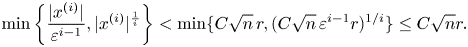
 \[ N_\varepsilon(x)= |x^{(1)}| + \sum_{i=2}^{\nu}\min\left\{\frac{|x^{(i)}|}{\varepsilon^{i-1}}, |x^{(i)}|^{\frac{1}{i}}\right\} \]
and for  $\varepsilon =0$ we set
 \[ N_0(x)= |x^{(1)}| + \sum_{i=2}^{\nu} |x^{(i)}|^{\frac{1}{i}} = \sum_{i=1}^{\nu} |x^{(i)}|^{\frac{1}{i}}. \]
The gauge  $N_\varepsilon$ is an adaptation of the gauge introduced in definition 3.9 in [Reference Capogna and Citti2].
Proposition 3.8 There exists a constant  $C\geq 1$ such that for all
  $\varepsilon \ge 0$ and
  $r>0$ we have
 \[ \{x\colon N_\varepsilon(x)< r \} \subset B_0^{\varepsilon}(0, C\ r), \]
and
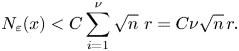
 \[ B_0^{\varepsilon}(0, r)\subset \{x\colon N_\varepsilon(x) < C\nu \sqrt{n}\ r \}. \]
Proof. Consider the case  $\varepsilon >0$. Suppose that
  $N_\varepsilon (x)< r$. We have
  $|x^{(1)}| < r$ and
  $\min \{\frac {|x^{(i)}|}{\varepsilon ^{i-1}}, |x^{(i)}|^{\frac {1}{i}}\}< r$ for indexes
  $i=2,\ldots \nu$. Observe that
 \[ \min\left\{\frac{|x^{(i)}|}{\varepsilon^{i-1}}, |x^{(i)}|^{\frac{1}{i}}\right\} = \left\{\begin{array}{ll} \dfrac{|x^{(i)}|}{\varepsilon^{i-1}} & \text{if}\ |x^{(i)}|\le \varepsilon^{i}\\ |x^{(i)}|^{\frac{1}{i}} & \text{if}\ |x^{(i)}|\ge \varepsilon^{i}, \end{array}\right. \]
so that we obtain
 \[ \min\left\{\frac{|x^{(i)}|}{\varepsilon^{i-1}} , |x^{(i)}|^{\frac{1}{i}} \right\} < r \implies \left\{\begin{array}{ll} \dfrac{|x^{(i)}|}{\varepsilon^{i-1}} < r & \text{if}\ r < \varepsilon\\ |x^{(i)}|^{\frac{1}{i}}< r & \text{if}\ r\ge \varepsilon. \end{array} \right. \]
In the case  $r<\varepsilon$ we get
  $|x^{(i)}|< \varepsilon ^{i-1} r$ that gives
  $x \in \text {Box}^{\varepsilon }(0,r)$. In the case
  $r\ge \varepsilon$ we get
  $|x^{(i)}|< r^{i}$ that gives
  $x\in \text {Box}(0,r)$. Using lemmas 3.2 and 3.4 we conclude that
  $x\in B_0^{\varepsilon }(0, C r)$ for some
  $C\ge 1$.
Suppose now that  $x\in B_0^{\varepsilon }(0,r)$. In the case
  $\varepsilon \geq r$, lemma 3.5 implies
  $x\in \text {Box}^{\varepsilon }(0, Cr)$ for some
  $C\geq 1$. We then have
  $|x^{(i)}| < C\sqrt {n}\, \varepsilon ^{i-1} r$,
  $i=1,\ldots , \nu$. We get
 \[ \min\left\{\frac{|x^{(i)}|}{\varepsilon^{i-1}}, |x^{(i)}|^{\frac{1}{i}}\right\} < \min\{ C\sqrt{n}\, r, (C\sqrt{n} \,\varepsilon^{i-1} r )^{1/i}\}\leq C\sqrt{n}r. \]
To achieve the last inequality above, notice that  $\varepsilon \geq C\sqrt {n}r$ implies
  $(C\sqrt {n} \,\varepsilon ^{i-1} r )^{1/i}\geq C\sqrt {n}r$, while
  $r\leq \varepsilon < C\sqrt {n}r$ implies
  $(C\sqrt {n} \,\varepsilon ^{i-1} r )^{1/i}< C\sqrt {n}r$.
In the case  $\varepsilon < r$, lemma 3.5 implies
  $x\in \text {Box}(0,Cr)$. We then have
  $|x^{(i)}| < \sqrt {n}\, C^{i} r^{i}$,
  $i=1,\ldots , \nu$. Hence, even in this case, we get
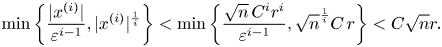 \[ \min\left\{\frac{|x^{(i)}|}{\varepsilon^{i-1}}, |x^{(i)}|^{\frac{1}{i}}\right\} < \min\left\{\frac{\sqrt{n}\, C^{i}r^{i}}{\varepsilon^{i-1}}, \sqrt{n}^{\frac{1}{i}}C\,r \right\}< C\sqrt{n}r. \]
Therefore, for all  $\varepsilon >0$, we obtain
 \[ N_\varepsilon(x)< C\sum_{i=1}^{\nu} \sqrt{n}\ r= C\nu \sqrt{n}\, r. \]
The case  $\varepsilon =0$ is just lemma 3.1.
Corollary 3.9 There exists a constant  $C\geq 1$ such that for all
  $\varepsilon \ge 0$ and
  $r>0$ we have
 \[ \frac{1}{C} d_0^{\varepsilon}(x,0)\le N_\varepsilon(x)\le C\nu \sqrt{n}\, d_0^{\varepsilon}(x,0). \]
4. The Poincaré and Sobolev inequalities
In this section we will use balls with an arbitrary, but fixed centre  $x_0$, so we simplify the notations for the average values over these balls as,
 \[ u_r = \unicode{x2A0D}_{B_0^{\varepsilon} (x_0,r)} u(x)\,{\rm d}x . \]
Lemma 4.1 Let  $\gamma : [0,1] \to {{\mathbb {G}}}$ be a
  $C^{1}$ curve such that
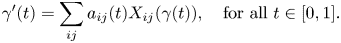 \[ \gamma' (t) = \sum_{ij} a_{ij} (t) X_{ij} (\gamma (t)),\quad \text{for all}\ t \in [0,1] . \]
If  $u \in C^{1} ({{\mathbb {G}}} )$, then we have
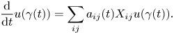 \[ \frac{{\rm d}}{{\rm d}t} u (\gamma (t)) = \sum_{ij} a_{ij}(t) X_{ij} u (\gamma (t)). \]
Proof. By definition, the derivative of a curve  $\gamma : [0,1] \to {{\mathbb {G}}}$ is the vector field defined as
  $\gamma '(t)\in T_{\gamma (t)}G$,
  $\gamma '(t)f=\frac {\textrm {d}}{\textrm {d}t}(f\circ \gamma )(t)$. If
  $\gamma ' (t) = \sum _{ij} a_{ij} (t) X_{ij} (\gamma (t))$ then it follows that
  $\frac {\textrm {d}}{\textrm {d}t} u (\gamma (t)) = \sum _{ij} a_{ij}(t) X_{ij} u (\gamma (t))$.
Let us recall the notation for the gradient relative to  ${{\mathcal {X}}}_1^{\varepsilon }$,
 \[ \nabla_0^{\varepsilon}u = \left(X_{11}u , \ldots , X_{1n_1}u, \, \varepsilon X_{21}u , \ldots, \varepsilon X_{2n_2}u, \, \ldots, \varepsilon^{\nu-1} X_{\nu 1} u , \ldots , \varepsilon^{\nu -1} X_{\nu n_{\nu}}u \right) , \]
which was already introduced in remark 2.9.
Our next theorem is the weak 1-1 Poincaré inequality for the balls  $B_0^{\varepsilon } (x,r)$. Note that the gradient appearing in the right-hand side of the inequality is the natural gradient along the approximating vector fields
  $\nabla _0^{\varepsilon } u$.
Theorem 4.2 There exists a constant  $C_1 \geq 1$, independent of
  $\varepsilon$, such that for all
  $u \in C^{1} ({{\mathbb {G}}} )$,
  $r>0$,
  $x_0 \in {{\mathbb {G}}}$ we have
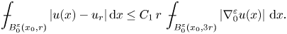 \[ \unicode{x2A0D}_{B_0^{\varepsilon} (x_0,r)} |u(x) - u_r|\,{\rm d}x \leq C_1 \, r \, \unicode{x2A0D}_{B_0^{\varepsilon} (x_0,3r)} \left| \nabla_0^{\varepsilon} u(x)\right|\,{\rm d}x. \]
The proof presented below shows that we can take
 \begin{equation} C_1 = 2n\,(c_d)^{2}\,3^{\log_2 {c_d}}, \end{equation}
where  $c_d$ is the doubling constant from theorem 3.6.
Proof. Let  $x, y \in B_0^{\varepsilon } (x_0,r)$ and
  $z \in {{\mathbb {G}}}$ such that
  $x=y \cdot z$. Then,
 \[ d_0^{\varepsilon}(z, 0) = d_0^{\varepsilon} (y^{{-}1} x, 0) = d_0^{\varepsilon} (x,y) < 2r. \]
By the left invariance of  $d_0^{\varepsilon }$ we have
  $d_0^{\varepsilon } (y\cdot z,y) < 2r$, so there exists
  $\varphi _{y,z} \in AC_0^{\varepsilon } (y, y \cdot z, 2r)$ such that
 \[ \varphi_{y,z}' (t) = \sum_{ij} a_{ij} (t)\, X_{ij} (\varphi (t)), \; \text{a.e.}\; t \in [0,1] \]
and
 \[ ||a^{(i)}||_{L^{\infty}([0,1], \mathbb{R}^{n_i})} < \varepsilon^{i-1} 2r ,\ 1 \leq i \leq \nu . \]
By lemma 4.1, we get that
 \[ u(y\cdot z) - u(y) = \int_0^{1} \frac{{\rm d}}{{\rm d}t} u(\varphi_{y,z} (t))\,{\rm d}t= \int_0^{1} \sum_{ij} a_{ij} X_{ij} u (\varphi_{y,z} (t))\,{\rm d}t. \]
Therefore, by embedding  $\varepsilon$ into
  $\nabla _0^{\varepsilon }$, we obtain that
 \[ |u(y\cdot z) - u(y) | \leq 2n r \int_0^{1} \left| \nabla_0^{\varepsilon} u (\varphi_{y,z} (t)) \right|{\rm d}t. \]
We use again the left invariance of  $d_0^{\varepsilon }$ and also the fact that the change of variables
  $x = y \cdot z$ has Jacobian equal to 1. Therefore,
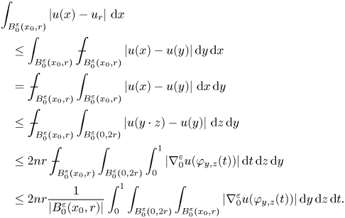 \begin{align*} & \int_{B_0^{\varepsilon} (x_0,r)} \left| u(x) - u_r \right|\,{\rm d}x \\ &\quad\leq \int_{B_0^{\varepsilon} (x_0,r)} \unicode{x2A0D}_{B_0^{\varepsilon} (x_0,r)} \left| u(x) - u(y) \right|{\rm d}y\,{\rm d}x\\ &\quad= \unicode{x2A0D}_{B_0^{\varepsilon} (x_0,r)} \int_{B_0^{\varepsilon} (x_0,r)} \left| u(x) - u(y) \right|\,{\rm d}x\,{\rm d}y \\ &\quad\leq \unicode{x2A0D}_{B_0^{\varepsilon} (x_0, r)} \int_{B_0^{\varepsilon}(0, 2r)} \left| u(y\cdot z) - u(y) \right|\,{\rm d}z\,{\rm d}y \\ &\quad\leq 2n r \unicode{x2A0D}_{B_0^{\varepsilon} (x_0 ,r)} \int_{B_0^{\varepsilon} (0, 2r)} \int_0^{1} \left| \nabla_0^{\varepsilon} u (\varphi_{y,z} (t) )\right|{\rm d}t\,{\rm d}z\,{\rm d}y\\ &\quad\leq 2n r \frac{1}{|B_0^{\varepsilon} (x_0 ,r)|} \int_0^{1} \int_{B_0^{\varepsilon} (0, 2r)} \int_{B_0^{\varepsilon} (x_0,r)} \left| \nabla_0^{\varepsilon} u (\varphi_{y,z} (t) )\right|{\rm d}y\,{\rm d}z\,{\rm d}t. \end{align*}
If  $\varphi _{y,z} \in AC_0^{\varepsilon } (y,y\cdot z, 2r)$, then there exists
  $\psi _{z} \in AC_0^{\varepsilon } (0,z,2r)$ such that
  $\varphi _{y,z} (t) = y \cdot \psi _{z} (t)$, for all
  $t \in [0,1]$. Therefore, if
  $y \in B_0^{\varepsilon } (x_0, r)$, then
 \begin{align*} d_0^{\varepsilon} (\varphi_{y,z}(t), x_0) & = d_0^{\varepsilon} (y \cdot \psi_z (t), x_0) \leq d_0^{\varepsilon} (y \cdot \psi_z (t), y) + d_0^{\varepsilon} (y, x_0)\\ &\leq d_0^{\varepsilon} (\psi_z (t) , 0) + d_0^{\varepsilon} (y , x_0) < 2r + r = 3r. \end{align*}
We continue the integral estimates started above.
 \begin{align*} &\int_{B_0^{\varepsilon} (x_0,r)} \left| u(x) - u_r \right|{\rm d}x \\ &\quad\leq 2n r \frac{1}{|B_0^{\varepsilon} (x_0 ,r)|} \int_0^{1} \int_{B_0^{\varepsilon} (0, 2r)} \int_{B_0^{\varepsilon} (x_0,r)} \left| \nabla_0^{\varepsilon} u (\varphi_{y,z} (t)) \right|{\rm d}y\,{\rm d}z\,{\rm d}t \\ &\quad= 2n r \frac{1}{|B_0^{\varepsilon} (x_0 ,r)|} \int_0^{1} \int_{B_0^{\varepsilon} (0, 2r)} \int_{B_0^{\varepsilon} (x_0,r)} \left| \nabla_0^{\varepsilon} u (y \cdot \psi_z (t)) \right|{\rm d}y\,{\rm d}z\,{\rm d}t\\ &\quad= 2n r \frac{1}{|B_0^{\varepsilon} (x_0 ,r)|} \int_0^{1} \int_{B_0^{\varepsilon} (0, 2r)} \int_{B_0^{\varepsilon} (x_0,r)\cdot \psi_z (t)} \left| \nabla_0^{\varepsilon} u (y_1)\right|dy_{1}\,{\rm d}z\,{\rm d}t\\ &\quad\leq 2n r \frac{1}{|B_0^{\varepsilon} (x_0 ,r)|} \int_0^{1} \int_{B_0^{\varepsilon} (0, 2r)} \int_{B_0^{\varepsilon} (x_0,3r)} \left| \nabla_0^{\varepsilon} u (y )\right|{\rm d}y\,{\rm d}z\,{\rm d}t\\ &\quad\leq 2n r \frac{|B_0^{\varepsilon} (0, 2r)|}{|B_0^{\varepsilon} (x_0 ,r)|} \int_{B_0^{\varepsilon} (x_0,3r)} \left| \nabla_0^{\varepsilon} u (y)\right|{\rm d}y. \end{align*}
Noting that, by theorem 3.6 we have
 \[ \frac{|B_0^{\varepsilon} (0, 2r)|}{|B_0^{\varepsilon} (x_0 ,r)|} = \frac{|B_0^{\varepsilon} (x_0, 2r)|}{|B_0^{\varepsilon} (x_0 ,r)|} \leq c_d , \]
we obtain
 \[ \int_{B_0^{\varepsilon} (x_0,r)} \left| u(x) - u_r \right|{\rm d}x \leq 2n \, c_d \, r \, \int_{B_0^{\varepsilon} (x_0,3r)} \left| \nabla_0^{\varepsilon} u (y) \right|{\rm d}y. \]
Finally, by corollary 3.7, we get
 \[ \unicode{x2A0D}_{B_0^{\varepsilon} (x_0,r)} \left| u(x) - u_r \right|{\rm d}x \leq C_1 \, r \, \unicode{x2A0D}_{B_0^{\varepsilon} (x_0,3r)} \left| \nabla_0^{\varepsilon} u (y )\right|{\rm d}y, \]
where
 \[ C_1 = 2n \,(c_d)^{2} \, 3^{\log_2 {c_d}} . \]
With the results of corollary 3.7 and theorem 4.2, we can use theorem 5.1 from [Reference Hajłasz and Koskela7], to get the Poincaré-Sobolev inequality:
Theorem 4.3 Let  $1 \leq p < Q$ and
  $1 \leq q \leq \frac {Qp}{Q-p}$. There exists a constant
  $C_{p,q} > 0$, independent of
  $\varepsilon$, such that for all
  $u \in C^{1} ({{\mathbb {G}}} )$,
  $r>0$,
  $x_0 \in {{\mathbb {G}}}$ we have
 \[ \left(\unicode{x2A0D}_{B_0^{\varepsilon} (x_0,r)} |u(x) - u_r|^{q}\,{\rm d}x \right)^{\frac{1}{q}} \leq C_{p,q}\, r \, \left(\unicode{x2A0D}_{B_0^{\varepsilon} (x_0,3r)} \left|\nabla_0^{\varepsilon} u(x) \right|^{p}\,{\rm d}x\right)^{\frac{1}{p}}. \]
Remark 4.4 We remark that the constant  $C_{p,q}$ in the above theorem is independent of
  $\varepsilon$ because, as detailed in theorem 5.1 of [Reference Hajłasz and Koskela7], it only depends on
  $p$,
$p$, $q$,
$q$,  $Q$, the constant
  $C_1$ of theorem 4.2 and the doubling constant
  $c_d$ of theorem 3.6, which are all independent of
  $\varepsilon$.
Remark 4.5 The balls  $B_0(x_0,r)$ and
  $B_0^{\varepsilon }(x_0, r)$ are John domains with constant
  $C=1$. Therefore, the Poincaré inequality from theorem 4.2 and the Poincaré-Sobolev inequality from theorem 4.3 hold with the same ball; that is, we can replace
  $B_0^{\varepsilon }(x_0, 3r)$ by
  $B_0^{\varepsilon }(x_0, r)$ in both inequalities by possibly changing the constants
  $C_1$ and
  $C_{p,q}$, which remain independent of
  $\varepsilon$. See § 9 in [Reference Hajłasz and Koskela7].
It is well-known that the Poincaré-Sobolev inequality implies the Sobolev inequality in our setting [Reference Hajłasz and Koskela7]. We use the notation  $C_0^{1} (B)$ for
  $C^{1}$ functions with compact support in
  $B$.
$B$.
Theorem 4.6 Let  $1 \leq p < Q$ and
  $1 \leq q \leq \frac {Qp}{Q-p}$. For all
  $r>0$,
  $x_0 \in {{\mathbb {G}}}$ and
  $u \in C_0^{1} (B_0^{\varepsilon } (x_0, r))$, we have
 \[ \left(\unicode{x2A0D}_{B_0^{\varepsilon} (x_0,r)} |u(x)|^{q}\,{\rm d}x \right)^{\frac{1}{q}} \leq C_{p,q}' \, r \, \left(\unicode{x2A0D}_{B_0^{\varepsilon} (x_0,r)} \left|\nabla_0^{\varepsilon} u(x) \right|^{p}\,{\rm d}x \right)^{\frac{1}{p}}, \]
where  $C_{p,q}'$ is a constant independent of
  $\varepsilon$.
In fact, keeping track of the constant we get
 \[ C_{p,q}'=\left(1+ 2 (c_d)^{\frac{1}{q}+1}\right)\, C_{p,q}, \]
where  $C_{p,q}$ is the Poincaré-Sobolev constant from theorem 4.3.
Remark 4.7 We remark that the main results of the paper continue to hold if instead of the Jacobian basis  $\{X_{ij}\}$ we choose any other basis
  $\{Y_{ij}\}$ adapted to the stratification, since we can pass from one to the other by multiplying by a suitable block diagonal matrix whose blocks are invertible matrices with constant entries.


