


1. Introduction
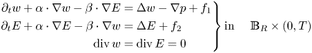
This paper is concerned with energy equality of the weak solution to the standard magneto-hydrodynamics (MHD) equations, for a velocity field $u$ , a magnetic field $B$
 and a pressure field $p$
 , as follows
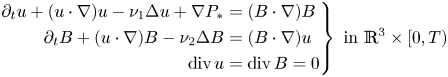
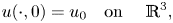
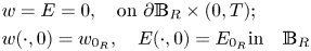
for any $T>0$ and the initial conditions

where $P_{\ast }=p+\frac {1}{2}|B|^{2}$ is the total pressure, and $\nu _{1},\,\nu _{2}>0$
 are coefficients of viscosity and coefficient of magnetic resistivity, respectively. The MHD equations are generally derived by coupling the Navier–Stokes equations for the velocity field of a fluid to Maxwell's equations governing the electric and magnetic fields (see, e.g., Duvaut–Lions [Reference Duvaut and Lions3]). Existence and uniqueness theory for MHD is closely related to that of the fundamental models of fluid mechanics, the Navier–Stokes equations

with the initial conditions
for which the global-in-time existence and uniqueness of smooth solutions is still a famous open problem. Similar to the the Navier–Stokes equations, a global weak solution (in the sense of definition 2.2) and local strong solution to (1.1) with the initial boundary value condition were constructed by Duvaut and Lions [Reference Duvaut and Lions3]. Later, these results were extended to the Cauchy problem (1.1) and (1.2) by Sermange and Teman [Reference Inria and Trmam11]. Here, their main tools are regularity theory of the Stokes operator and the energy method.
It is well known that the concept of kinetic energy becomes particularly important in existence and uniqueness theory of models of fluid mechanics, starting with the fact that Leray [Reference Leray13] and Hopf [Reference Hopf10] prove the existence of the weak solution to the Navier–Stokes equations (1.3) and (1.4). Because the boundedness of kinetic energy provides a primary a priori estimate, it allows us to construct a weak solution (called nowadays Leray–Hopf weak solutions when we are restricted under Navier–Stokes equations), and such weak solutions satisfy energy inequality. The energy inequality can be regarded as weak solutions lacking sufficient regularity, actually, if weak solution has sufficient regularity, it can satisfy the equal sign in the energy inequality, i.e., energy equality. The classical result in this direct go back to the Lions [Reference Lions15], which shows that if $u$ is a weak solution to the Navier–Stokes equations (1.3) and (1.4) in addition to satisfying

then necessarily $u$ obeys
obeys

Subsequently, Lions's result was extended to the general case by Shinbrot [Reference Shinbort20], precisely, they proved if

then (1.6) is still valid, where their argument relies on the regularity result of Serrin [Reference Serrin19], which sates that a Leray–Hopf weak solution $u$ is regular, furnished the following criterion holds
Recently, Galdi [Reference Galdi6] improved Lion's result by a mollifying procedure and a duality argument. Precisely, he showed that if $u\in L_\textrm {loc},\,\sigma ^{2}(\mathbb {R}^{3}\times (0,\,T))$ is a very weak solution (for details, please see definition 2.3), and satisfies (1.5), then necessarily $u$
 obeys the energy equality (1.6). Later, Galdi's result was extended to the general case (1.7) by Berselli–Chiodaroli [Reference C. Berselli and Chiodaroli1].
Turning to the standard 3D MHD equations, there is a large body of work on various regularity criteria. For example, He-Xin[Reference He and Xin9] proved that if $(u,\,B)$ is a weak solution of (1.1), and $u$
 satisfies (1.8), then $(u,\,B)$
 is smooth in $\mathbb {R}^{3}\times (0,\,T]$
 , and of course it satisfies the related energy equality:

for all $0< t\leq T$ . For more results in this field, please see [Reference Chen, Miao and Zhang2, Reference He and Xin8, Reference Luo, Zhao and Yang16, Reference Miao, Yuan and Zhang17, Reference Wu21]. However, there is a little literature on energy conservation criteria for the standard MHD equations, the only reference, to our knowledge, is [Reference Kim12] where the author proved if the pair $(u,\,B)$
 is a weak solution of the MHD equations and $(u,\,B)$
 fulfills energy conservation criteria (1.7), then the energy equality (1.9) holds.
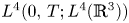
In the present paper, we, inspired by the argument of Galdi [Reference Galdi6], will extend energy conservation criteria of Galdi to MHD equations, and prove that if $(u,\,B)\in L^{4}(0,\,T;L^{4}(\mathbb {R}^{3}))$ is a very weak solution to (1.1), then it is actually in the Leray–Hopf class. Thus the energy equality (1.9) holds. The main result of the present paper is stated as
Theorem 1.1 Let $u_{0},\,B_{0}\in L_{\sigma }^{2}(\mathbb {R}^{3}),$ and the pair $(u,\,B)\in L_{loc}^{2}(\mathbb {R}^{3}\times (0,\,T))$
 be a very weak solution of (1.1) in the sense of definition 2.3. If $u,\,B$
 are in $L^{4}(0,\,T;L^{4}(\mathbb {R}^{3})),$
 then the very weak solution pair $(u,\,B)$
 is, actually, in the Leray–Hopf class. Thus it obeys the energy equality (1.9).
The rest paper of this paper is organized as follow. In § 2, we give some preliminaries. Section 3 presents the detailed proof of our main results. Finally, the energy conservation theorem of weak solution to the standard MHD equation (1.1) is provided in appendix A.
2. Preliminaries
2.1 Functional spaces
Let $T>0$ and let $\mathbf {X}$
 be a Banach space. We shall consider $L^{p}(0,\,T;\mathbf {X}),\,1\!\leq p\!\leq \infty$
 , which is the space of functions from $[0,\,T]$
 into $\mathbf {X}$
 , which are $\textrm {L}^{p}$
 for the Lebesǵue measure $\textrm {d}t$
 . This is a Banach space endowed with the norm

For simplicity, we write $\|\cdot \|_{L^{p}(\mathbb {R}^{3})}=\|\cdot \|_{p}$ when $\Omega =\mathbb {R}^{3}$
 . And the space $W^{k,p}(\Omega )$
 is the usual Sobolev space, if $u\in W^{k,p}(\Omega )$
 we define its norm by

As usual, we write $W^{1,2}(\Omega )=H^{1}(\Omega ),\,W_{0}^{1,2}(\Omega )=H_{0}^{1}(\Omega )$ . Besides, we give the following spaces which are usually used when one investigates the mathematical theory of Navier–Stokes equations:

Finally, we define $t$ -anisotropic Sobolev spaces

Usually, one denotes by

the Stokes operator in $\Omega$ , where

is the Helmholtz–Leray projection given by

when $\Omega =\mathbb {R}^{n}$ , and $\Delta _{D}$
 is the Laplace operator under the Dirichlet boundary condition. The domain of Stokes operator is $D(A)=H_{0,\sigma }^{1}(\Omega )\cap W^{2,2}(\Omega )$
 .
.
Next we give a basic theorem, which will be used in our proof.
Theorem 2.1 [Reference Robinson, Rodrigo and Sadowski18]
Let $\Omega$ be a smooth bounded domain in $\mathbb {R}^{3}$
 . Then there exists a family of functions $\mathcal {N}=\{a_{1},\,a_{2},\,a_{3},\,\cdots \}$
 such that
(i) $\mathcal {N}$
 is an orthogonal basis in $L_{\sigma }^{2}(\Omega );$
(ii) $a_{j}\in D(A)\cap C^{\infty }(\overline {\Omega })$
are eigenfunctions of the Stokes operator, that is $Aa_{j}=\lambda _{j}a_{j}$ for all $j\in \mathbb {N}$ with
\[ 0<\lambda_{1}\leq\lambda_{2}\leq\lambda_{3}\leq\cdots\leq\lambda_{j}\leq\cdots \quad and \quad \lambda_{j}\rightarrow\infty; \](iii) $\mathcal {N}$
is an orthogonal basis in $H_{0,\sigma }^{1}(\Omega ).$


2.2 The definition of weak solutions, the form $\mathfrak {B}_{0}$ and the operator $\mathfrak {B}$


First, we present the notion of energy weak solution of (1.1).
Definition 2.2 The pair $(u,\,B)\in L^{\infty }(0,\,T;L_{\sigma }^{2}(\mathbb {R}^{3}))\cap L^{2}(0,\,T;W^{1,2}(\mathbb {R}^{3}))$ is called as energy weak solution in $\mathbb {R}^{3}\times (0,\,T)$
 if
if
(1) The pair $(u,\,B)$
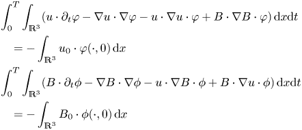
solves (1.1) in the distribution sense
(2.2)\begin{equation} \begin{aligned} & \int_{0}^{T}\int_{\mathbb{R}^{3}}(u\cdot\partial_{t}\varphi-\nabla u\cdot\nabla\varphi-u\cdot\nabla u\cdot\varphi+B\cdot\nabla B\cdot\varphi)\,\textrm{d}x\textrm{d}t\\ & \quad ={-}\int_{\mathbb{R}^{3}}u_{0}\cdot\varphi({\cdot},0)\,\textrm{d}x\\ & \int_{0}^{T}\int_{\mathbb{R}^{3}}(B\cdot\partial_{t}\phi-\nabla B\cdot\nabla\phi-u\cdot\nabla B\cdot\phi+B\cdot\nabla u\cdot\phi)\,\textrm{d}x\textrm{d}t\\ & \quad ={-}\int_{\mathbb{R}^{3}}B_{0}\cdot\phi({\cdot},0)\,\textrm{d}x \end{aligned} \end{equation}for all $\varphi,\,\phi \in \mathcal {D}_{T}$ and $u_{0},\,B_{0}\in L_{\sigma }^{2}(\mathbb {R}^{3})$.(2) Such solution pair $(u,\,B)$
satisfies the energy inequality
(2.3)\begin{equation} \|u(t)\|_{2}^{2}+\|B(t)\|_{2}^{2}+2\int_{0}^{t}(\|\nabla u(\tau)\|_{2}^{2}+\|\nabla B(\tau)\|_{2}^{2})\,\textrm{d}\tau\leq (\|u_{0}\|_{2}^{2}+\|B_{0}\|_{2}^{2}) \end{equation}for all $0< t< T$.


In the present paper, the main goal is to consider the energy equality of very weak solutions to (1.1). To this end, we give the definition of very weak solutions of (1.1) as follows
Definition 2.3 We say that the pair $(u,\,B)\in L_{loc,\sigma }^{2}(\mathbb {R}^{3}\times (0,\,T))$ is a very weak solution of equation (1.1), if
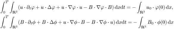
for some $u_{0},\,B_{0}\in L_{\sigma }^{2}(\mathbb {R}^{3})$ and all $\varphi,\,\phi \in \mathcal {D}_{T}$
 .
.
Remark 2.4 In fact, denote by $\Gamma =(u,\,B),\,\Gamma _1=(B,\,u)$ and $\Psi =(\varphi,\,\phi )$
 , we can rewrite (2.4) as

with $\Gamma _{0}=(u_0,\,B_0),\, \Psi _0=(\varphi (x,\,0),\,\phi (x,\,0))$ .
.
In order to deal with nonlinear term conveniently, we introduce a trilinear form $\mathfrak {B}_{0}$ . First, we define now a trilinear form on $(H_{0}^{1}(\Omega ))^{3}$
 by setting

whenever the integral makes sense. Actually, from Hölder inequality and embedding theorem,

so $b$ is a trilinear continuous form on $(H_{0}^{1}(\Omega ))^{3}$
 . In particular, if $u\in H_{0,\sigma }^{1}(\Omega )$
 , we can easily get by a direct calculation

and

In order to write (2.5) as a simpler form, we define a trilinear form $\mathfrak {B_{0}}$ on $(H_{0,\sigma }^{1}(\Omega ))^{3}$
 as
as

for all $\Phi ^{1},\,\Phi ^{2},\,\Phi ^{3}\in H_{0,\sigma }^{1}(\Omega )$ . Here

Due to the continuous $b$ , one derives that $\mathfrak {B_{0}}$
 is trilinearly continuous on $(H_{0,\sigma }^{1}(\Omega ))^{3}$
 . This let us give a continuous bilinear operator $\mathfrak {B}$
 from $H_{0,\sigma }^{1}(\Omega )\times H_{0,\sigma }^{1}(\Omega )$
 into $(H_{0,\sigma }^{1}(\Omega ))^{'}$
 as
as

The definition of $\mathfrak {B}_{0}$ , along with (2.6) and (2.7), gives

This yields an alternative form of weak formulation (2.5) as follows, which will be used in the proof of the lemma 3.1. Precisely, if we choose $\varphi,\,\phi \in C_{0,\sigma }^{\infty }(\mathbb {R}^{3})$ , one can rewrite (2.2) as

with $(f,\,g)=\int _{\mathbb {R}^{3}}f\cdot g \,\textrm {d}x$ , then this system can be equivalently rewritten as

Using the operators $A$ and $\mathfrak {B}$
 perviously defined, (2.10) is equivalent to the following formula
i.e., (2.10) is a weak formulation of the problem (2.11).
Next we will introduce the standard mollifying techniques which will be used in the proof of our main results. Let $\epsilon >0$ be a sufficiently small parameter, we define space and space-time mollifiers of $h$
 with $h\in L^{1}_\textrm {{loc}}(\mathbb {R}^{3}\times [0,\,T))$
 , respectively, by

where

with $j\in C_{0}^{\infty }(-\epsilon,\,\epsilon )$ and $k\in C_{0}^{\infty }(\mathbb {R}^{3})$
 .
.
We conclude this section by introducing an essential lemma, which ensures that the divergence of the approximate sequence is also zero when we approximate the sequence to the initial condition of the divergence of zero.
Lemma 2.5 For any $v\in H^{1}(\mathbb {R}^{3})\cap L_{\sigma }^{2}(\mathbb {R}^{3}),$ one can find an approximation sequence $v_{R}\in H_{0}^{1}(\mathbb {B}_{R})\cap L_{\sigma }^{2}(\mathbb {B}_{R}),$
 where $\mathbb {B}_{R}$
 is the ball with the origin as the centre and $R$
 as the radius, and

Proof. Let $\psi \in C^{1}(\mathbb {R})$ be a cut-off function with $\psi (\xi )\!=\!1$
 if $|\xi |\!\leq 1$
 , $\psi (\xi )=0$
 if $|\xi |\!\geq 2$
 and set $\psi ^{R}(x)=\psi (\frac {|x|}{R})$
 . From [Reference Galdi5], we can get an unique solution $w_{R}\in H_{0}^{1}(\mathbb {B}_{R,2R})$
 (where $\mathbb {B}_{R,2R}=\{x| R<|x|<2R\}$
 ) to the problem

and $w_{R}$ satisfies

with the constant $c$ independent of $R$
 . Moreover, since $\nabla \psi ^{R}=\mathcal {O}(\frac {1}{R})$
 uniformly in $x$
 , using Poincaré inequality and (2.12), one can get

Then we set $w_{R}\equiv 0$ in the complement of $\mathbb {B}_{R,2R}$
 and define

it is easy to check $\overline {v}\in H_{0,\sigma }^{1}(\mathbb {B}_{2R})$ . Next, for any given $\epsilon \geq 0$
 , we can acquire a sequence $\overline {v}^{(\epsilon )}\in C_{0,\sigma }^{\infty }(\Omega _{2R})$
 due to the mollifying techniques such that

Therefore,

Because of (2.13) and the properties of $\psi ^{R}$ , when $R$
 is sufficiently large and $\epsilon$
 is sufficiently small, we can make the right side of this inequality as small as we please, namely,

Similarly, by (2.12) and the properties of $\psi ^{R}$ , when $R$
 sufficiently large and $\epsilon$
 sufficiently small, one can obtain

So, we can choose $v_{R}=\overline {v}^{(\epsilon )}$ , which completes the proof of this lemma.
3. Proof of theorem 1.1
To prove theorem 1.1, we first consider the following regularize problem related to equation (1.1)
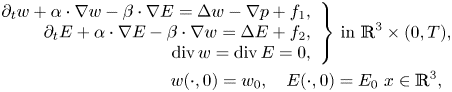
where $\alpha,\,\beta \in C_{0,\sigma }^{\infty }([0,\,T)\times \mathbb {R}^{3}),\, w_{0},\,E_{0}\in L_{\sigma }^{2}(\mathbb {R}^{3})$ and $f_{1},\,f_{2}\in C_{0}^{\infty }((0,\,T)\times \mathbb {R}^{3})$
 with some $T>0$
 . Note that using the same method as in remark 2.4, we can rewrite equation (3.1) as

where $\Phi =(w,\,E)$ , $f=(f_{1},\,f_{2})$
 , $\Theta =(\alpha,\,\beta )$
 and $A$
 is the Stokes operator defined in (2.1).
By a standard Galerkin technique, we can construct a energy weak solution of (3.1). If $\Phi$ is a weak solution in a bounded domain $\Omega \subset \mathbb {R}^{3}$
 guarantees that at each time $t>0$
 the function $\Phi (t)$
 is an element of the infinite-dimensional space $L_{\sigma }^{2}$
 spanned by the eigenfunctions of the Stokes operator. The Galerkin method allows us to construct a weak solution $\Phi$
 as the limit of approximate solutions $\Phi _{n}$
 that each time $t>0$
 belongs to the finite-dimensional space $P_{n}L_{\sigma }^{2}$
 spanned by the first $n$
 eigenfunctions,

Here $\mathcal {N}$ is the basis given in theorem 2.1 and by $P_{n}$
 we denote the projection operator $P_{n}:L^{2}\rightarrow L_{\sigma }^{2}$
 defined by

More precisely, we have the following technical lemma which plays a key role in our proof of theorem 1.1.
Lemma 3.1
(i) If $(w_{0},\,E_{0})\in L_{\sigma }^{2}(\mathbb {R}^{3}),$
the Cauchy problem (3.1) exists a unique solution pair $(w,\,E)$ such that
(3.4)\begin{equation} (w,E)\in L^{\infty}(0,T;L_{\sigma}^{2}(\mathbb{R}^{3}))\cap L^{2}(0,T;W^{1,2}(\mathbb{R}^{3})), \end{equation}moreover(3.5)\begin{equation} \begin{aligned} & \max_{t\in [0,T]}(\|w(t)\|_{2}^{2}+\|E(t)\|_{2}^{2})+\int_{0}^{T}(\|\nabla w(t)\|_{2}^{2}+\|\nabla E(t)\|_{2}^{2})\,\textrm{d}t\\ & \quad \leq\|w_{0}\|_{2}^{2}+\|E_{0}\|_{2}^{2}+c_{0}\int_{0}^{T}(\|f_{1}(t)\|_{\frac{6}{5}}^{2}+\|f_{2}(t)\|_{\frac{6}{5}}^{2})\,\textrm{d}t \end{aligned} \end{equation}with some positive constant $c_{0}$.(ii) $($
Improved regularity.$)$ If $(w_{0},\,E_{0})\in H^{1}(\mathbb {R}^{3})\cap L_{\sigma }^{2}(\mathbb {R}^{3}),$ then
(3.6)\begin{equation} w,E\in W^{2,1}_{2,T}\subset C(0,T;H^{1}(\mathbb{R}^{3})). \end{equation}In addition, if $w_{0},\,E_{0}\equiv 0,$ we have also $(w,\,E)\in W^{2,1}_{4/3,T}\times W^{2,1}_{4/3,T}\times L^{\frac {4}{3}}(0,\,T; L^{4/3}(\mathbb {R}^{3}))$.


Proof. (i) We will prove the related result by using the standard Galerkin technique. Let $\mathbb {B}_{R}\subset \mathbb {R}^{3}$ be the ball of radius $R$
 centred at the origin, we consider the following problem
endowed with the initial-boundary value condition
where $w_{0_{R}},\,E_{0_{R}}\in L_{\sigma }^{2}(\mathbb {B}_{R})$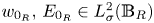 obey
obey

Here the existence of $w_{0_{R}},\,E_{0_{R}}$ can be ensured by lemma 2.5. Similarly, (3.7) can be equivalently written as
with

According to (3.9) we also have
In the following, we will invoke the classical Galerkin method, coupled with ‘invading domains’ technique to explore the existence of solutions for (3.10) in the class of (3.4).
Step 1. In this step, we will prove that the system (3.10) admits a solution at least locally in time. To this end we consider the problem


for the form of functions $\Phi _{n}$ and $\Theta _{n}$

where $a_{k}(x)\in \mathcal {N}$ is the basis of $L^{2}(\mathbb {B}_{R})$
 . To determine $\Phi _{n}$
 we need to find the functions $c_{k}^{n}(t)$
 . To get the desired result, we take the inner product of (3.12) in $L^{2}$
 with $a_{k}$
 , $k=1,\,2,\,\cdots n$
 . Since $( P_{n}v,\,a_{k})=( v,\,a_{k})$
 for every $v\in L^{2}(\mathbb {R}^{3})$
 and $1\leq k\leq n$
 , one derives

Using the fact that the $a_{k}$ are eigenfunctions of the Stokes operator and are orthonormal in $L^{2}(\mathbb {B}_{R})$
 we therefore obtain a system of ODEs,

where

and $\widehat {c}_{i}^{n}(t)=(\Theta _{n},\,a_{i})$ is the coefficients of $\Theta _{n}$
 . To find initial conditions for $c_{k}^{n}$
 we take the inner product of (3.13) with $a_{k}$
 , which yields

From the classical theory of ODEs, one immediately obtains (3.14) admits a unique solution $(c_{1}^{n},\,\cdots,\, c_{n}^{n})$ on some time interval $[0,\,T_{n})$
 , from which we obtain the corresponding solution $\Phi _{n}$
 of (3.12).
Step 2. We obtain uniform estimates on the solutions $\Phi _{n}$ and hence show that $T_n=T$
 . We already know that $\Phi _{n}$
 exists at least on some time interval $[0,\,T_{n})$
 . Let $s\in (0,\,T_{n})$
 , we take the inner product of (3.12) with $\Phi _{n}(s)$
 to get

On the one hand,

and

On the other hand, the nonlinear term vanishes due to the definition of operator $\mathfrak {B}$ and $\textrm {div}\ \Theta _{n}=0$
 , i.e.,

Therefore for all $s>0$ we have
Now, integrating (3.15) from $0$ to $t$
 , for all $t\in [0,\,T_n)$
 , along with (3.11), Sobolev inequality and Cauchy–Schwartz inequality, yields

with $C$ independent of $t$
 and $n$
 . In particular, (3.16) shows that $|c_{k}^{n}(t)|\leq C^{\frac{1}{2}}$
 for all $k=1,\,\cdots,\,n$
 and $t\in [0,\,T_n)$
 which in turn, by a standard technique on ordinary differential equations, implies that the $c_{k}^{n}$
 do not blow up at $t=T_n$
 and hence $T_{n}=T$
 . In addition, from (3.16) we get
and hence

Therefore we have shown that the approximate solution sequence $\Phi _{n}$ is bounded uniformly in $L^{\infty }(0,\,T;L^{2}(\mathbb {B}_{R}))\cap L^{2}(0,\,T;H_{0,\sigma }^{1}(\mathbb {B}_{R}))$
 .
.
Step 3. We establish the uniform bounds on $\partial _{t}\Phi _{n}$ in $L^{2}(0,\,T;(H_{0,\sigma }^{1}(\mathbb {B}_{R}))^{'})$
 . For any $\varphi \in H_{0,\sigma }^{1}(\mathbb {B}_{R})$
 , we take the $L^{2}$
 inner product of the Galerkin equation (3.12) with $\varphi$
 to obtain

To estimate the norm $\|\partial _{t}\Phi _{n}\|_{(H_{0,\sigma }^{1}(\mathbb {B}_{R}))^{'}}$ , we need to estimate each term of the right-hand side of the above equality. It is clear that

for some smooth $\tilde {\varphi }$ . On the other hand, by Hölder inequality and the Sobolev embedding theorem

and

Therefore,

with the constant $c$ independent of $n$
 . From this, one immediately derives

where in the last inequality we have used the inequality (3.16).
Step 4. We extract a convergent subsequence and pass to the limit in the equation. From step 2, there exists an absolute constant $C$ such that

Therefore, by Aubin–Lions Lemma [Reference Robinson, Rodrigo and Sadowski18, theorem 4.3] one can find a subsequence of $\{\Phi _{n}\}$ ( we still denote by $\{\Phi _{n}\}$
 ) such that

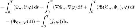
We now show that $\Phi _{R}$ is a weak solution of equation (3.10). It is enough to check that for any fixed $\varphi \in \mathcal {D}_{T}$
 we have
If we take the dot product of (3.12) with $\varphi$ , and integrate in space, then integrating the second term by part yield, we get

Integrating in $[0,\,T)$ and using integrating by parts in the first term we obtain that
We pass to limit in (3.21), as $n\rightarrow \infty$ . From the convergence (3.18) and (3.19) we have

and
To prove that

we notice that

Hence we need to show that

and

From the bound (3.17) it follows that

Moreover, from the weak convergence of gradients in (3.19) it follows that

as $n\rightarrow \infty$ for all $1\leq i,\,j\leq 3$
 , as $\Theta _{j}\varphi _{i}\in L^{2}$
 . Hence

Therefore we obtain (3.20).
Step 5. We prove that (3.1) exists at least one weak solution.
From steps 1–4, we can find a weak solution $\Phi _{R}$ of the equations (3.10). We extend the functions $\Phi _{R}$
 by zero outside $\mathbb {B}_{R}$
 and still denote such extended functions by $\Phi _{R}$
 . Note that due to the zero boundary conditions these extended functions belong to $H_{0,\sigma }^{1}(\mathbb {R}^{3})$
 for almost every time $t$
 . The sequence $\{\Phi _{R}\}$
 of weak solutions shares many properties with the sequence of Galerkin approximations considered in the step 1–4. In particular, it follows from our method of construction that we have a uniform bound

with some constant independent of $R$ . From the above bound we conclude that for some subsequence of $\{\Phi _{R}\}$
 (which we relabel)

for some $\Phi \in L^{2}(0,\,T;W^{1,2}(\mathbb {R}^{3}))$ . Furthermore, for all $R>1$
 the estimates on the time derivative in step 3 shows

for some $C>0$ independent of $R$
 . Since $(H_{0,\sigma }^{1})^{'}(\mathbb {B}_{R})\subset (H_{0,\sigma }^{1})^{'}(\mathbb {B}_{M})$
 for all $R\geq M$
 with
with

then we have for all $R\geq M$

Thus, by Aubin–Lions Lemma, for every $M\in \mathbb {N}$ we can find a subsequence of $\{\Phi _{R}\}$
 which converges strongly in $L^{2}(0,\,T;L_{\sigma }^{2}(\mathbb {B}_{M}))$
 . Using the standard diagonal argument we can choose a subsequence of $\{\Phi _{R}\}$
 , still denoted by $\{\Phi _{R}\}$
 , such that

for every $M=1,\,2,\,3\cdots$ . It remains to show that the limit function $\Phi$
 is a weak solution of the equation (3.1). To do this, take any test function $\phi \in \mathcal {D}_{T}$
 where the support of $\phi$
 is contained in $\mathbb {B}_{M}\times [0,\,T)$
 for a large enough $M$
 . Then for all $R>M$
 we have

where we have used the fact that $\Phi _{R}$ is a weak solution of the equation (3.7) in $\mathbb {B}_{R}\times [0,\,T)$
 and $\phi \in \mathcal {D}_{T}(\mathbb {B}_{R})$
 . We pass to the limit as $R\rightarrow \infty$
 using the weak convergence of $\nabla \Phi _{R}$
 and strong convergence of $\Phi _{R}$
 in $L^{2}(0,\,T;L^{2}(\mathbb {B}_{M}))$
 , and prove that $\Phi$
 is a weak solution of the equation (3.1) with the initial $\Phi _{0}$
 .
.
(ii) To improve the regularity of the solution, multiplying both sides of (3.12) by $\mathbb {P}\Delta \Phi _{n}$ , and integrating by parts the resulting relations over $\mathbb {B}_{R}$
 , one derives

i.e.,

where we have used the fact $\Theta \in L^{\infty }(0,\,\infty,\,L^{\infty }(\mathbb {R}^{3}))$ . From this, one immediately obtains

This, along with Gronwall's inequality, yields for all $t\in [0,\,T]$

Here, we have used the fact that $\|\nabla \Phi _{n}(0)\|_{2}^{2}<\|\Phi _{0_{R}}\|_{H^{1}(\mathbb {B}_{R})}<\infty$ . Next, we integrate both sides of (3.22) from $0$
 to $t$
 , to gain

Similar as above, dot-multiplying both sides of (3.12) by $\partial _{t}\Phi _{n}$ , one can gain
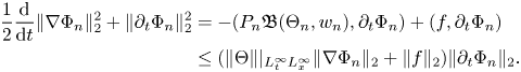
Using Gronwall's inequality again, we get

This, together with (3.11), (3.16), and the well-known estimate

with a constant $C$ independent of $R$
 (for details, please see [Reference Heywood7]), implies

where the constant $C$ depends only on $T$
 , $f$
, $f$ , $\|\Theta \|_{L_{t}^{\infty }L_{x}^{\infty }}$
 , and $\|\Phi _{0}\|_{2}$
 and is therefore independent of $n$
 . Therefore, (3.24) implies $\Phi \in W^{2,1}_{2,T}$
 , and from the classical interpolation result in [Reference Lions14] we can get $W^{2,1}_{2,T}\subset C([0,\,T];H^{1}(\mathbb {R}^{3}))$
 .
.
Now, we consider the case $\Phi _{0}\equiv 0$ . By Hölder inequality, (3.16) and $\Theta \in L^{4}(0,\,T;L^{4}(\mathbb {R}^{3}))$
 , we have

which implies, in particular, that

Therefore, from classical results of [Reference Galdi5, theorem VIII.4.1], the problem

with $F=\mathfrak {B}(\Theta,\, \Phi )+f$ , has at least one solution $\overline {\Phi }$
 such that

However, by uniqueness of Stokes operator, see, for example, [Reference Galdi5, lemma VIII.4.2], we must have $\Phi \equiv \overline {\Phi }$ , which completes the proof of this lemma.
We are now in a position to show theorem 1.1.
Proof of theorem 1.1. Proof of theorem 1.1
To obtain the desired result, we, in equations (3.2), first take

and

where $u,\,B,\,u_{0},\,B_{0}$ are defined in Theorem 1.1. By lemma 3.1, equations (3.2) admits a solution $\Phi _{\epsilon }=(w_{\epsilon },\,E_{\epsilon })\in W^{2,1}_{2,T}$
 which fulfills for any pair $(\varphi,\,\phi )\in \mathcal {D}_{T}$
From (2.4) and (3.26) we infer that

Using the same method as in remark 2.4, for any $\Psi =(\varphi,\,\phi )\in \mathcal {D}_{T}$ , we can write the above two equalities as

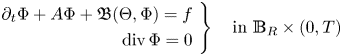
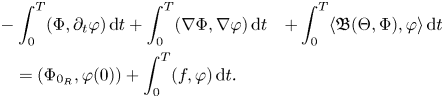
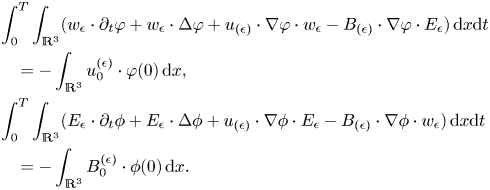
On the other hand, according to lemma 3.1, the duality equation

with

admits a solution $\overline {\Phi }_{\epsilon }\in W^{2,1}_{4/3,T}\cap W^{2,1}_{2,T}$ . Now let $\Lambda _{\epsilon }(x,\,t)=\overline {\Phi }_{\epsilon }(T-t,\,x)$
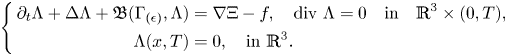
 , then it solves the final-value problem
On the other hand, from the fact that $\mathcal {D}_{T}$ is dense in $\dot {W}_{q,T}^{1,2}:=\!\{u\!\in\! W_{q,T}^{1,2},\, u(\cdot,\,T)\!=\!0\}$
 , for details please see [Reference Galdi6, lemma A.1], we can take $\Psi =\Lambda _{\epsilon }$
 in (3.27) and use (3.28)1 to deduce

Here we have used the fact $\int _{0}^{T}((\Gamma -\Phi _{\epsilon }),\,\nabla \Xi _{\epsilon })\, \textrm {d}t=0$ due to $\mbox {div}\,\Gamma =\mbox {div}\,\Phi _{\epsilon }=0$
 .
.
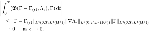
In what follows, we need to pass to the limit $\epsilon \rightarrow 0$ in (3.29) to finish our proof. Indeed, by (3.5),

with some constant $C$ independent of $\epsilon$
 . From this, we immediately derive

Secondly,
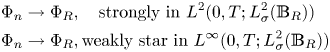
On the other hand, by (3.5), we can find a subsequence of $\{\Phi _{\epsilon }\}$ , still denoted by $\{\Phi _{\epsilon }\}$
 , such that as $\epsilon \to 0$

for some $\Phi \in L^{\infty }(0,\,T;L_{\sigma }^{2}(\mathbb {R}^{3}))\cap L^{2}(0,\,T;W^{1,2}(\mathbb {R}^{3}))$ . From this, we immediately gain
for any $f\in C_{0}^{\infty }(\mathbb {R}^{3}\times (0,\,T))$ . Finally, from (3.29)–(3.32) we conclude that

which in turn, by the arbitrariness of $f$ , implies $\Gamma =\Phi$
 . Therefore,

then by theorem A.2, $\Gamma =(u,\,B)$ obeys the energy equality (1.9) in the time interval $[0,\,T]$
 .
.
Appendix A. Energy equality of weak solutions of the MHD equations
In this part, we will give a proof of the energy equality of weak solution to the MHD equations, for reader's convenience. Before starting the proof, we give a technical lemma as follows.
Lemma A.1 Assume $\Phi$ be a weak solution of (1.1) with the initial value $\Phi _{0}\in L^{2}(\mathbb {R}^{3})$
 . Then $\Phi$
 can be redefined on a set of zero Lebesgue measure in such a way that $\Phi (\cdot,\, t)\in L^{2}(\mathbb {R}^{3})$
 for all $t\in [0,\,T)$
 and satisfies the identity

for all $\Psi \in \mathcal {D}_{T}$ .
.
The proof of this lemma can be found in, such as, [Reference Galdi4, Reference Shinbort20].
Now we present the following theorem, which is about the energy equality of weak solutions of the MHD equations. Although its proof is classical, we can not find it in the literature. I will present its proof for reader's convenience.
Theorem A.2 Let $\Phi _{0}=(u_{0},\,B_{0})\in L_{\sigma }^{2},$ and let $\Phi =(u,\,B)$
 be a weak solution of (1.1) and (1.2). In addition,

then $\Phi$ satisfies the energy equality

for all $t\in [0,\,T]$ .
.
Proof. Let ${\Phi ^{i}}=(u^{i},\,B^{i})\subset \mathcal {D}_{T}$ be a sequence such that

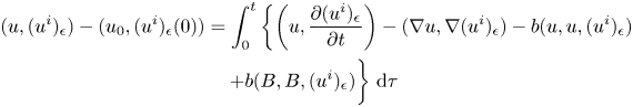
Thus, we can choose $\Psi (t)=(\Phi ^{i})_{\epsilon }(t)$ in (A.1), where $(\cdot )_{\epsilon }$
 is the standard time mollifying operator, i.e. $(\Phi ^{i})_{\epsilon }(t)=\int _{0}^{T}j_{\epsilon }(t-s)\Phi ^{i}(s)\textrm {d}s$
 . Then, from lemma A.1 one has

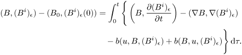
i.e.,
and
Note that, (2.7), along with the Hölder inequality and the interpolation inequality, shows that when $i\rightarrow \infty$

where we have used the fact $u\in L^{\infty }(0,\,T;L_{\sigma }^{2}(\mathbb {R}^{3}))\cap L^{2}(0,\,T;W^{1,2}(\mathbb {R}^{3}))\cap L^{r}(0,\,T;L^{s}(\mathbb {R}^{3}))$ . Similarly, we can also get when $i\rightarrow \infty$

and $|\int _{0}^{t}b(B,\,u,\,(B^{i})_{\epsilon }-B_{\epsilon })\,\textrm {d}\tau |\rightarrow 0$ . Therefore, let $i$
 tend to infinity in (A.4) and (A.5), one has

In what follows, we need to pass to the limit $\epsilon \rightarrow 0$ in (A.6) to finish our proof. In fact, from the fact $j_{\epsilon }$
 is even in $(-\epsilon,\,\epsilon )$
 and the basic properties of mollifiers,
and

Besides, the weak $L^{2}$ continuity of weak solution, along with the fact $\int _{0}^{\epsilon }j_{\epsilon }s)\textrm {d}s=\frac {1}{2}$
 , implies

Similarly, we also have when $\epsilon \rightarrow 0$

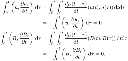
Now we turn to the nonlinear term in (A.6). Indeed, a simple calculation shows as $\epsilon \rightarrow 0$

Here, we have used the fact

Similarly, as $\epsilon \rightarrow 0$

Thus, let $\epsilon \rightarrow 0$ in (A.6), we deduce

This, along with the definition of $\mathfrak {B}_{0}$ , yields

Since $\Phi (\cdot,\, t)=(u(\cdot,\,t),\,B(\cdot,\,t))\in H_{\sigma }^{1}(\mathbb {R}^{3})$ for a.e $t$
 , we get by an approximation technique

From which the desired result is obtained.
Acknowledgments
We thank the anonymous referee for constructive comments which helped to improve the paper. This work is supported in part by the National Natural Science Foundation of China under grant No. 11971148.
