


1. Introduction
In this article, we study the existence of positive solutions of the following semilinear elliptic problem with Hardy–Sobolev critical exponent:
 \begin{align}
\left.\begin{array}{lr}
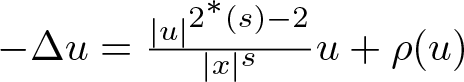
\quad -\Delta u = \frac{|u|^{2^{*}(s)-2}u}{|x|^s}+ \rho(u) \, \text{in}\, \Omega \\
\quad \quad u \gt 0\quad \mbox{in}\, \Omega,\quad u = 0 \, \mbox{in}\, \partial\Omega
\end{array}
\right\},
\end{align}
\begin{align}
\left.\begin{array}{lr}
\quad -\Delta u = \frac{|u|^{2^{*}(s)-2}u}{|x|^s}+ \rho(u) \, \text{in}\, \Omega \\
\quad \quad u \gt 0\quad \mbox{in}\, \Omega,\quad u = 0 \, \mbox{in}\, \partial\Omega
\end{array}
\right\},
\end{align} where Ω is a bounded smooth domain in  $\mathbb R^n$ with
  $0\in \Omega$,
  $0 \lt s \lt 2$,
  $2^{*}(s)$ is the Hardy–Sobolev critical exponent
  $2^{*}(s)= \frac{2(n-s)}{n-2}$ and
  $\rho : \mathbb R\rightarrow \mathbb R$ is a given function. It follows from a standard use of Pohozaev identity that the above problem does not have a solution when ρ = 0 and Ω is star shaped. When ρ is a linear perturbation
  $\rho(u) = \lambda u$ the problem does admit solutions for
  $0 \lt \lambda \lt \lambda_1$ when
  $n\ge 4$ in the spirit of the well-known Brézis–Nirenberg problem, where λ 1 is the first eigenvalue of the Laplacian in Ω with Dirichlet boundary conditions (see theorem 1.3 in [Reference Ghoussoub and Yuan8]).
In this article, we will analyse the existence of least energy solutions under certain assumptions on the perturbation ρ and study its necessity for the existence of least energy solutions. The case s = 0 was analysed in detail in [Reference Adimurthi and Sandeep1]. The main objective of this article is to show that when s > 0 we would not see some of the phenomenon observed in [Reference Adimurthi and Sandeep1] for the case s = 0 for lowering the energy, which we will explain below. We consider perturbation  $\rho \in C^1(\mathbb R)$ which satisfy
  $\rho(0)=\rho^{\prime}(0)=0$,
  $\rho^{\prime}$ bounded and
  $\rho(t)=0(t^{-b})$ as
  $t\rightarrow \infty$ for some b > 0 and our aim is to find conditions on ρ which yield solutions with least energy.
First recall that a solution of (1.1) is a function  $u\in H^1_0(\Omega)$ satisfying
 \begin{align}
\int_{\Omega}\nabla u \cdot \nabla v \ dx \ = \ \int_{\Omega}
\frac{|u|^{2^{*}(s)-2}uv}{|x|^s}\ dx + \ \int_{\Omega}\rho(u)v\ dx
\end{align}
\begin{align}
\int_{\Omega}\nabla u \cdot \nabla v \ dx \ = \ \int_{\Omega}
\frac{|u|^{2^{*}(s)-2}uv}{|x|^s}\ dx + \ \int_{\Omega}\rho(u)v\ dx
\end{align} for all  $v\in H^1_0(\Omega)$, and u > 0, i.e., the solutions are the positive critical points of the energy functional
 \begin{align}
J(u) \ =\ \frac{1}{2}\int_{\Omega}|\nabla u|^2 dx -\frac{1}{2^*(s)}\int_{\Omega}\frac{(u^+)^{2^*(s)}}{|x|^s} dx -\int_{\Omega} \tilde{\rho}(u^+) dx \ , \ u\in H^1_0(\Omega)
\end{align}
\begin{align}
J(u) \ =\ \frac{1}{2}\int_{\Omega}|\nabla u|^2 dx -\frac{1}{2^*(s)}\int_{\Omega}\frac{(u^+)^{2^*(s)}}{|x|^s} dx -\int_{\Omega} \tilde{\rho}(u^+) dx \ , \ u\in H^1_0(\Omega)
\end{align} where  $\tilde{\rho}(t) = \int\limits_0^t\rho(s)\ ds.$ The energy functional is well defined on
  $H^1_0(\Omega)$ thanks to the Hardy–Sobolev inequality:
 \begin{align}
\int_{\mathbb{R}^n} |\nabla u|^2\ dx \ \ge \ A_s\left(\int_{\mathbb{R}^n}\frac{|u|^{2^{*}(s)}}{|x|^s} \right)^{\frac{2}{2^*(s)}}\ , \ u\in C_c^1(\Omega)
\end{align}
\begin{align}
\int_{\mathbb{R}^n} |\nabla u|^2\ dx \ \ge \ A_s\left(\int_{\mathbb{R}^n}\frac{|u|^{2^{*}(s)}}{|x|^s} \right)^{\frac{2}{2^*(s)}}\ , \ u\in C_c^1(\Omega)
\end{align} where  $A_s \gt 0$ is the optimal constant in the above inequality, depending only on n and s. It is also known that extremal of the above inequality exists in the space
  $D^{1,2}(\mathbb R^n)$ which is the completion of
  $C_c^\infty (\mathbb R^n)$ with the norm
  $\left(\int_{\mathbb{R}^n} |\nabla u|^2\ dx \right)^{\frac{1}{2}}.$ Moreover, the extremal up to a constant satisfies the PDE:
 \begin{align}
\left.
\begin{array}{l}
-\Delta u \ = \ \frac{u^{2^{*}(s)-1}}{|x|^s} \ \ {\rm in}\ \mathbb R^n \\
u \gt 0 ,\ \ \int_{\mathbb{R}^n} |\nabla u|^2\ dx \ \lt \ \infty
\end{array}
\right\}.
\end{align}
\begin{align}
\left.
\begin{array}{l}
-\Delta u \ = \ \frac{u^{2^{*}(s)-1}}{|x|^s} \ \ {\rm in}\ \mathbb R^n \\
u \gt 0 ,\ \ \int_{\mathbb{R}^n} |\nabla u|^2\ dx \ \lt \ \infty
\end{array}
\right\}.
\end{align}Classification of solutions of (1.5) and the exact value of As is known (see [Reference Chou and Chu3], [Reference Ghoussoub and Yuan8]).
The main difficulty in proving the existence of a solution for the problem (1.1) is the lack of compactness of the associated energy functional J. More precisely, J does not satisfy the Palais–Smale condition in general. In fact, if u is any solution of (1.5) and  $\epsilon_m \gt 0$ with
  $\epsilon_m \rightarrow 0$ as
  $m\rightarrow\infty$ then the sequence defined by
  $u_m = (\epsilon_m)^{-\frac{n-2}{2}}u(\frac{x}{\epsilon_m})$ is a Palais–Smale sequence for J at level
  $\frac{2-s}{2(n-s)} A_s^{\frac{n-s}{2-s}}$. However, one can show that either the problem (1.1) has a solution or J satisfies the Palais–Smale condition in the interval
  $\left(0, \frac{2-s}{2(n-s)} A_s^{\frac{n-s}{2-s}}\right).$ Therefore, the strategy is to find a Palais–Smale sequences at level
  $C \in \left(0, \frac{2-s}{2(n-s)} A_s^{\frac{n-s}{2-s}}\right).$ It is well known that for similar problems in lower dimensions the positive mass (positivity of the Robin function at a point) is crucial in obtaining this (see [Reference Druet4], [Reference Schoen13]). However, in higher dimensions, the perturbation ρ does have an impact in getting the Palais–Smale (PS) level as evident from the case s = 0 which was well studied in [Reference Brézis and Nirenberg2] and further analysed in [Reference Adimurthi and Sandeep1].
In [Reference Brézis and Nirenberg2], Brézis and Nirenberg showed that when  $\rho \not= 0$ is compactly supported and non-negative then (1.1) has a solution u satisfying
  $J(u) \lt \frac{A_0^{\frac{n}{2}}}{n}$. In fact, the same arguments show that when ρ is compactly supported and real valued then the problem (1.1) has a solution u satisfying
  $J(u) \lt \frac{A_0^{\frac{n}{2}}}{n}$ if either
  $\int_{\mathbb R^n} \tilde{\rho}\left(\frac{1}{|x|^{n-2}}\right) \gt 0$ and
  $n\geq 5$ or
  $n\ge 7$ and
  $\int_{\mathbb R^n} \tilde{\rho}\left(\frac{1}{|x|^{n-2}}\right)=0$ and
  $\int_{\mathbb R^n} \rho\left(\frac{1}{|x|^{n-2}}\right)\frac{1}{|x|^{n}} dx \lt 0$. These results were proved by using the standard bubbles (extremal of Sobolev inequality) as test functions. However, it was shown in [Reference Adimurthi and Sandeep1] that these conditions are not sharp when
  $n\ge 7$. In fact, in [Reference Adimurthi and Sandeep1], an almost necessary and sufficient condition was discovered for the existence of solution for the problem with the energy bound. These results were proved by using a different class of test functions incorporating the effect of ρ which are perturbations of standard bubbles. This phenomenon discovered in [Reference Adimurthi and Sandeep1] was shown to be true in many other cases, like the case of bi-Laplace equation with critical growth (see [Reference Robert and Sandeep12]).
The aim of this article is to show that this phenomenon of a modified test function lowering the energy when standard bubbles fail does not occur for (1.1) when  $0 \lt s \lt 2$. More precisely, the standard bubbles yield the optimal result when s > 0 unlike the case s = 0. Before we state our main results, let us define:
Definition 1.1. We say that a solution of (1.1) is of the least energy if it satisfies  $J(u) \lt \frac{(2-s)}{2(n-s)} A_s^{\frac{n-s}{2-s}}$, where J is the energy defined in (1.3).
With this definition, we can state our main results. First, we establish the necessary conditions for the existence of least energy solution in all balls.
Theorem 1.2. Let  $n\ge 5$,
  $\rho\in C^1(\mathbb R)$ be such that
  $\rho(0)=\rho^{\prime}(0)=0$,
  $\rho^{\prime}$ bounded and
  $\rho(t)=0(t^{-b})$ as
  $t\rightarrow \infty$ for some
  $b \gt \max\left\{0, \frac{2(1-s)}{n-2}\right\}$. Assume that (1.1) has a least energy solution on
  $B(0,R)$ for any R > 0 , then
  $ \int_{0}^{\infty} \tilde{\rho}(t) t^{-\frac{2(n-1)}{n-2}} dt \ge 0$. If
  $ \int_{0}^{\infty} \tilde{\rho}(t) t^{-\frac{2(n-1)}{n-2}} dt = 0$, then
  $\int_{0}^{\infty}{\rho(t)}{t^{-\frac{n-2+s}{n-2}}} dt \le 0.$
Remark 1.3. The above theorem tells us that if  $n\ge 5$ and ρ satisfies
  $ \int_{0}^{\infty} \tilde{\rho}(t) t^{-\frac{2(n-1)}{n-2}} dt = 0$, and
  $\int_{0}^{\infty}{\rho(t)}{t^{-\frac{n-2+s}{n-2}}} dt \gt 0$, then (1.1) does not have a least energy solution for
  $0 \lt s \lt 2$. However, this is not true for s = 0, there are perturbations ρ which satisfy the above conditions with s = 0 for which least energy solutions do exist (see [Reference Adimurthi and Sandeep1]).
Our next theorem shows that the existence does hold if we have strict inequalities in the necessary conditions given in the previous theorem, making the conditions almost necessary and sufficient for the existence of least energy solutions in all balls.
Theorem 1.4. Let Ω is a bounded domain in  $\mathbb R^n$ with smooth boundary containing the origin in its interior,
  $\rho\in C^1(\mathbb R)$ such that
  $\rho(0)=\rho^{\prime}(0)=0$,
  $\rho^{\prime}$ bounded and
  $\rho(t)=0(t^{-b})$ as
  $t\rightarrow \infty$ for some
  $b \gt \max\left\{0, \frac{2(1-s)}{n-2}\right\}$. Then (1.1) with s > 0 admits a least energy solution under any of the following two assumptions:
(i)
 $\int_{0}^{\infty} \tilde{\rho}(t) t^{-\frac{2(n-1)}{n-2}} dt \gt 0$ if
$n\geq 5$,
$\int_{0}^{\infty} \tilde{\rho}(t) t^{-\frac{2(n-1)}{n-2}} dt \gt 0$ if
$n\geq 5$,(ii)
$\int_{0}^{\infty} \tilde{\rho}(t) t^{-\frac{2(n-1)}{n-2}} dt = 0$ and
$ \int_{0}^{\infty}{\rho(t)}{t^{-\frac{n-2+s}{n-2}}} dt \lt 0$ if
$n \gt 6-s$.


It is possible to establish the existence of a solution even in more general cases under the assumption (i) of previous theorem, see, for example, [Reference Adimurthi and Sandeep1], [Reference Dutta5].
This article is arranged as follows: In §2, we will prove the regularity properties of solutions and recall the associated Hardy–Sobolev inequality and the classification of positive solutions of the corresponding Euler–Lagrange equation. In §3, we will do a blow-up analysis of least energy solutions in small balls in the lines of the analysis in [Reference Adimurthi and Sandeep1]. In §4 and §5, we will prove our main theorems.
Notations: Throughout the article, all integrals are with respect to the Lebesgue measure and we will denote by  $\| \cdot \|$ the L 2 norm of the function involved.
The spaces  $H^2(\Omega)$ and
  $H^2_0(\Omega)$ will denote the standard L 2 Sobolev spaces.
The space  $D^{1,2}(\mathbb R^n)$ will denote the completion of
  $C_c^\infty (\mathbb R^n)$ with the norm
  $\left(\int_{\mathbb{R}^n} |\nabla u|^2\ dx \right)^{\frac{1}{2}}.$
The standard terms ‘big o’ and ‘small o’ indicating the asymptotic behaviour of quantities will be denoted by O and o respectively.
The surface measure of the unit sphere in  $\mathbb R^n$ will be denoted by
  $\omega_{n-1}$.
2. Preliminaries and basic lemmas
In this section, we will look at in detail the smoothness of solutions and symmetry properties and also recall the classification of solutions of the limiting problem (1.5) and some basic estimates.
2.1. Regularity and symmetry of solutions
First recall that we have defined the solution of (1.1) as a weak solution as in (1.2). Then, it immediately follows from standard elliptic theory that  $u\in C^2_{loc}(\overline{\Omega} \setminus \{0\})$. We will show below that the solution is in fact Hölder continuous in Ω for any
  $0 \lt s \lt 2.$
Theorem 2.1. Let u be a weak solution of (1.1) then  $ u\in C^{\alpha}(\overline{\Omega})$ for some
  $\alpha \in (0,1)$.
Proof. The Hölder continuity will follow from corollary 4.23 of [Reference Han and Lin10] if we show that the weak solution is bounded as  $\frac{1}{|x|^s} \in L^{q}(B(0,R))$ for some
  $q \gt \frac{n}{2}$. As observed before, enough to prove the boundedness in a neighbourhood of 0 which will follow from theorem 8 of [Reference Ghoussoub and Robert7] (by applying γ = 0) or following the Moser iteration scheme as done in lemmas 3.1 and 3.2 of [Reference Mancini, Fabbri and Sandeep11] (
 $|y| $ replaced by
  $|x|$).
 $\square$
Next we show that if Ω is a ball, then any solution of (1.1) is radial. The result will follow from the moving plane method, by suitably adapting the arguments of [Reference Gidas, Ni and Nirenberg9] and [Reference Terracini15]. We will only outline the proof.
Theorem 2.2. Let Ω be a ball of radius R > 0 and ρ be Lipschitz, then any solution of (1.1) is radial and radially decreasing.
Proof. Without loss of generality we may assume  $\Omega = B := \{x : |x| \lt R\}$ and define for
  $0\le \lambda \lt R$,
  $B_\lambda = \{x=(x_1,\ldots ,x_n)\in B : \lambda \lt x_1 \lt R\}$ and
  $T_\lambda = \{x\in B : x_1=\lambda\}$. For
  $x\in B_\lambda$ denote its reflection with respect to Tλ by
  $x^\lambda := (2\lambda-x_1,x_2,\ldots, x_n)$ and define
  $u_\lambda(x) = u(x^\lambda)$ for
  $x\in B_\lambda$. First we show that
  $u_\lambda(x) \ge u(x)$ for all
  $x\in B_\lambda$ when λ is close to R.
Define  $w_\lambda = u-u_\lambda$ then using the equation u satisfies and the fact that
  $|x^\lambda| \lt |x|$ for
  $x\in B_\lambda$ we see that wλ satisfies
 \begin{align*} -\Delta w_\lambda \le A(x)\frac{w_\lambda}{|x|^s} +B(x)w_\lambda \, {\rm in} \, B_\lambda,\, w_\lambda \in H^1(B_\lambda), \, w_\lambda \le 0 \, {\rm on}\, \partial B_\lambda \end{align*}
 where  $A(x):=0$ when
  $u(x)=u_\lambda(x)$, otherwise
 \begin{align*} 0\le A(x) := \frac{u^{2^\ast(s)-1}(x)- u_\lambda^{2^\ast(s)-1}(x)}{u(x) -u_\lambda(x)} \le (2^\ast(s)-1)\left[ \max{u(x),u_\lambda(x)}\right]^ {2^\ast(s)-2}\end{align*}
 and  $|B(x)| \le L$ where L is the Lipschitz constant of ρ.
Multiplying the inequality by  $w_\lambda^+$ and integrating by parts, we get
 \begin{align*}\int_{B_\lambda}|\nabla w_\lambda^+ |^2 \le \int_{B_\lambda} A(x)\frac{(w_\lambda^+)^2}{|x|^s} + \int_{B_\lambda}B(x)(w_\lambda^+)^2.\end{align*}
Applying the Cauchy–Schwartz inequality, the Hardy–Sobolev inequality (1.4), and the standard Sobolev inequality, the above inequality becomes
 \begin{align*}\int_{B_\lambda}|\nabla w_\lambda^+ |^2 \le C\left[ \left( \int_{B_\lambda\cap \{u \gt u_\lambda \}} \frac{A(x)^{\frac{n-s}{2-s}}}{|x|^s}\right)^{\frac{2-s}{n-s}} + \left( \int_{B_\lambda}|B(x)|^{\frac n2}\right)^{\frac 2n} \right] \int_{B_\lambda}|\nabla w_\lambda^+ |^2. \end{align*}
 Now using the bounds  $|B|\le L$ and
  $|A(x)| \le (2^\ast(s)-1)u(x)^ {2^\ast(s)-2}$ in the region of integration, we see that the term in square bracket on the RHS goes to zero as
  $\lambda \rightarrow R.$ Thus, there exists a
  $\lambda_0 \in (0,R)$ such that
  $u_\lambda \ge u$ in Bλ for all
  $\lambda \in (\lambda_0,R)$.
Let  $A = \{\lambda_0 \in (0,R) : u_\lambda \ge u \, {\rm in}\, B_\lambda \, {\rm for \, all}\, \lambda \in (\lambda_0,R) \}$ and
  $\Lambda:= \inf A$. We claim that
  $\Lambda =0$. Let
  $\Lambda \gt 0$, we will show that this will contradict the definition of Λ. First note that by continuity
  $w_\Lambda \le 0$ in
  $B_\Lambda$ and
  $w_\Lambda $ solves
  $ \Delta w_\Lambda +B(x)w_\Lambda \ge 0 \, {\rm in} \, B_\Lambda$. If
  $\Lambda \gt \frac R2$, then
  $w_\Lambda$ is also
  $C^2(\overline{B_{\Lambda}})$ and so by strong maximum principle
  $w_\Lambda \gt 0$ in
  $B_\Lambda$. Hence using standard arguments, we can show that there exists a
  $\Lambda_0 \lt \Lambda$ such that
  $u_\lambda \ge u$ in Bλ for all
  $\lambda \in (\Lambda_0,R)$ gives a contradiction. If
  $\Lambda \le \frac R2$, then
  $w_\Lambda$ is in
  $C^2(\overline{B_\Lambda}\setminus \{(2\Lambda,0,\ldots,0)\})$ and hence by strong maximum principle
  $w_\Lambda \gt 0$ in
  $B_\Lambda \setminus \{(2\Lambda,0,\ldots,0)\}.$ Again by using a small measure type arguments near the singularity
  $(2\Lambda,0,\ldots,0)$, combining with the positivity of
  $w_\Lambda$ we can get a contradiction. For details of these types of arguments, we refer to the proof of theorem 2.1 in [Reference Mancini, Fabbri and Sandeep11]. Thus, we get
  $u(-x_1,\ldots,x_n) \ge u(x_1,\ldots,x_n)$ for
  $x_1 \gt 0$. Similarly moving the plane from the left, we get the opposite inequality and hence symmetry in the x 1 direction. Rest of the proof is standard and we omit the details.
 $\square$
2.2. Limiting problem
We know that when s = 0, the Euler–Lagrange equation of the Sobolev inequality is the limiting problem and its solutions play a crucial role in the analysis of (1.1) with s = 0. When s > 0, the limiting problem will be (1.5). We will recall below the classification of its solutions.
Define  $U : \mathbb R^n \rightarrow \mathbb R$ and
  $U_\epsilon :\mathbb R^n \rightarrow \mathbb R$ for ϵ > 0 by
 \begin{align} U(x)=\left[\frac{a}{a+|x|^{2-s}}\right]^{\frac{n-2}{2-s}} \, {\rm and} \,\, U_{\epsilon}(x)=\frac{1}{\epsilon^{\frac{n-2}{2}}}U\left(\frac{x}{\epsilon}\right)=\left[\frac{a\epsilon^{\frac{2-s}{2}}}{a\epsilon^{2-s}+|x|^{2-s}}\right]^{\frac{n-2}{2-s}},
\end{align}
\begin{align} U(x)=\left[\frac{a}{a+|x|^{2-s}}\right]^{\frac{n-2}{2-s}} \, {\rm and} \,\, U_{\epsilon}(x)=\frac{1}{\epsilon^{\frac{n-2}{2}}}U\left(\frac{x}{\epsilon}\right)=\left[\frac{a\epsilon^{\frac{2-s}{2}}}{a\epsilon^{2-s}+|x|^{2-s}}\right]^{\frac{n-2}{2-s}},
\end{align} where  $a= (n-2)(n-s)$. Then by direct calculation, we see that Uϵ solves
 \begin{align}
\left.\begin{array}{lr}
- \Delta U_{\epsilon} = \frac{|U_\epsilon|^{2^{*}(s)-1}}{|x|^s}\,\mbox{in}\, \mathbb R^n\\
\int_{\mathbb R^n}|\nabla U_{\epsilon}|^2 = \int_{\mathbb R^n}\frac{U_{\epsilon}^{2^*(s)}}{|x|^s}= A_s^{\frac{n-s}{2-s}}
\end{array}
\right\},
\end{align}
\begin{align}
\left.\begin{array}{lr}
- \Delta U_{\epsilon} = \frac{|U_\epsilon|^{2^{*}(s)-1}}{|x|^s}\,\mbox{in}\, \mathbb R^n\\
\int_{\mathbb R^n}|\nabla U_{\epsilon}|^2 = \int_{\mathbb R^n}\frac{U_{\epsilon}^{2^*(s)}}{|x|^s}= A_s^{\frac{n-s}{2-s}}
\end{array}
\right\},
\end{align}where As is the best constant in (1.4). Moreover, we have the following classification result (see [Reference Ghoussoub and Yuan8], [Reference Chou and Chu3]):
Theorem 2.3. Let u be a solution of (1.5), then  $u=U_\epsilon$ for some ϵ > 0.
We also need the following estimates on Uϵ, we omit their proof as it follows by direct calculation (see [Reference Ghoussoub and Yuan8]).
Lemma 2.4. Let R > 0 be fixed, Uϵ be as in (2.1). Then we have the following:
 \begin{align}
\begin{aligned}
\nabla U_{\epsilon}(x)&=- (n-2) \frac{1}{a\epsilon^{\frac{2-s}{2}}} \left[\frac{a\epsilon^{\frac{2-s}{2}}}{a\epsilon^{2-s}+ |x|^{2-s}}\right]^{\frac{n-s}{2-s}} |x|^{-s} x. \\
\int_{B(R)}|\nabla U_{\epsilon}|^2 &= A_s^{\frac{n-s}{2-s}} +O\left(\epsilon^{n-2}\right).\end{aligned}\qquad\qquad\quad\;\;
\end{align}
\begin{align}
\begin{aligned}
\nabla U_{\epsilon}(x)&=- (n-2) \frac{1}{a\epsilon^{\frac{2-s}{2}}} \left[\frac{a\epsilon^{\frac{2-s}{2}}}{a\epsilon^{2-s}+ |x|^{2-s}}\right]^{\frac{n-s}{2-s}} |x|^{-s} x. \\
\int_{B(R)}|\nabla U_{\epsilon}|^2 &= A_s^{\frac{n-s}{2-s}} +O\left(\epsilon^{n-2}\right).\end{aligned}\qquad\qquad\quad\;\;
\end{align} \begin{align}
\int_{B(R)} \frac{U_{\epsilon}^{2^{*}(s)}}{|x|^s} = A_s^{\frac{n-s}{2-s}} + O\left(\epsilon^{n-s}\right).\qquad\qquad\qquad\qquad\qquad\qquad\qquad\qquad
\end{align}
\begin{align}
\int_{B(R)} \frac{U_{\epsilon}^{2^{*}(s)}}{|x|^s} = A_s^{\frac{n-s}{2-s}} + O\left(\epsilon^{n-s}\right).\qquad\qquad\qquad\qquad\qquad\qquad\qquad\qquad
\end{align} \begin{align}
\int_{B(R)} \frac{U_{\epsilon}^{\beta}}{|x|^s} = \left\{
\begin{array}{lr}
\epsilon^{n-s-\beta\left(\frac{n-2}{2}\right)}\left[O(1)+O\left(\epsilon^{(n-2)\beta -n+s}\right)\right] & \mbox{if}\, \beta\ne \frac{n-s}{n-2}\\
O\left(\epsilon^{n-s-\left(\frac{n-2}{2}\right)\beta}\log \epsilon \right) & \mbox{if}\, \beta = \frac{n-s}{n-2}.
\end{array}\right.
\end{align}
\begin{align}
\int_{B(R)} \frac{U_{\epsilon}^{\beta}}{|x|^s} = \left\{
\begin{array}{lr}
\epsilon^{n-s-\beta\left(\frac{n-2}{2}\right)}\left[O(1)+O\left(\epsilon^{(n-2)\beta -n+s}\right)\right] & \mbox{if}\, \beta\ne \frac{n-s}{n-2}\\
O\left(\epsilon^{n-s-\left(\frac{n-2}{2}\right)\beta}\log \epsilon \right) & \mbox{if}\, \beta = \frac{n-s}{n-2}.
\end{array}\right.
\end{align}Next we collect some estimates which easily follow from (2.1) and (2.5).
Lemma 2.5. The following hold
 \begin{align}
\qquad\;\;\;\;\;\qquad\int_{B(1)} \frac{U_{\epsilon}^{\frac{n+2-2s}{n-2}}}{|x|^s} U_{\epsilon}(1) = o(1)\epsilon^{\frac{n-2}{2}}.
\end{align}
\begin{align}
\qquad\;\;\;\;\;\qquad\int_{B(1)} \frac{U_{\epsilon}^{\frac{n+2-2s}{n-2}}}{|x|^s} U_{\epsilon}(1) = o(1)\epsilon^{\frac{n-2}{2}}.
\end{align} \begin{align}
\;\, \int_{B(1)} \frac{(U_{\epsilon}+|U_{\epsilon}(1)|)^{\frac{n+2-2s}{n-2}}}{|x|^s} U_{\epsilon}(1) = o(1)\epsilon^{\frac{n-2}{2}}.
\end{align}
\begin{align}
\;\, \int_{B(1)} \frac{(U_{\epsilon}+|U_{\epsilon}(1)|)^{\frac{n+2-2s}{n-2}}}{|x|^s} U_{\epsilon}(1) = o(1)\epsilon^{\frac{n-2}{2}}.
\end{align} \begin{align}
\int_{B(1)} \frac{(U_{\epsilon}+ |U_{\epsilon}(1)|)^{\frac{4-2s}{n-2}} }{|x|^s}(U_{\epsilon}(1))^2 = o(1)\epsilon^{n-2}.
\end{align}
\begin{align}
\int_{B(1)} \frac{(U_{\epsilon}+ |U_{\epsilon}(1)|)^{\frac{4-2s}{n-2}} }{|x|^s}(U_{\epsilon}(1))^2 = o(1)\epsilon^{n-2}.
\end{align}3. Blow-up analysis of least energy solutions
Throughout this section, we assume ρ satisfies  $\rho\in C^1(\mathbb R),\ \rho(0)=\rho^{\prime}(0)=0$,
  $\rho^{\prime}$ bounded and
  $\rho(t)=0(t^{-b})$ as
  $t\rightarrow \infty$ for some
  $b \gt \max\left\{0, \frac{2(1-s)}{n-2}\right\}$.
Assume that (1.1) has a least energy solution on any ball in  $\mathbb R^n$, for some
  $n\geq 5$. Let uR be a least energy solution of (1.1) with
  $\Omega = B(R):= B(0,R)$ for R > 0.
Define for R > 0,  $V_R: B(1)\rightarrow \mathbb R$ by
 \begin{align*}V_{R}= R^{\frac{n-2}{2}} u_{R}(R x)\ , \ \ x\in B(1).\end{align*}
Then VR satisfies
 \begin{align}
\left.\begin{array}{l}
-\Delta V_{R} = \frac{V_{R}^{2^*(s)-1}}{|x|^s} + R^{\frac{n+2}{2}} \rho\left(\frac{V_{R}(x)}{R^{\frac{n-2}{2}}}\right)\,\mbox{in}\, B(1)\\
V_{R} \gt 0\,\mbox{in}\,B(1),\quad V_{R}= 0\,\mbox{on}\,\partial B(1)
\end{array}
\right\},
\end{align}
\begin{align}
\left.\begin{array}{l}
-\Delta V_{R} = \frac{V_{R}^{2^*(s)-1}}{|x|^s} + R^{\frac{n+2}{2}} \rho\left(\frac{V_{R}(x)}{R^{\frac{n-2}{2}}}\right)\,\mbox{in}\, B(1)\\
V_{R} \gt 0\,\mbox{in}\,B(1),\quad V_{R}= 0\,\mbox{on}\,\partial B(1)
\end{array}
\right\},
\end{align}and the least energy condition becomes
 \begin{align}
J_{R}(V_R) & =\frac{1}{2}\int_{B(1)} |\nabla V_{R}|^2 -\frac{1}{2^{*}(s)}\int_{B(1)} \frac{|V_{R}|^{2^{*}(s)}}{|x|^s} \nonumber\\
& \quad - R^{n} \int_{B
(1)} \tilde{\rho}\left(\frac{V_R}{R^{\frac{n-2}{2}}}\right) \lt \frac{2-s}{2(n-s)}A_s^{\frac{n-s}{2-s}}.
\end{align}
\begin{align}
J_{R}(V_R) & =\frac{1}{2}\int_{B(1)} |\nabla V_{R}|^2 -\frac{1}{2^{*}(s)}\int_{B(1)} \frac{|V_{R}|^{2^{*}(s)}}{|x|^s} \nonumber\\
& \quad - R^{n} \int_{B
(1)} \tilde{\rho}\left(\frac{V_R}{R^{\frac{n-2}{2}}}\right) \lt \frac{2-s}{2(n-s)}A_s^{\frac{n-s}{2-s}}.
\end{align}Moreover, VR is radially decreasing thanks to theorem 2.2.
The main aim of this section is to establish the following decomposition of VR:
Theorem 3.1. There exists an  $R_0 \gt 0$ such that for every
  $0 \lt R \lt R_0$, VR can be decomposed as
 \begin{align*}V_R= a_R\left(U_{\epsilon_R} - U_{\epsilon_R}(1)\right) + E_R \end{align*}
 where  $\epsilon_{R} \gt 0$,
  $\epsilon_R\rightarrow 0$ as
  $R\rightarrow 0$ and
  $U_{\epsilon_R}$ is as defined in (2.1). Also
  $a_R \gt 0$ and
  $\epsilon_R \gt 0$ satisfy the following estimate
 \begin{align*}1-a_{R} = o\left(\epsilon_R^{\frac{n-2}{2}}\right), \, \,
\|\nabla E_{R}\| = o\left(\epsilon_R^{\frac{n-2}{2}}\right).\end{align*}
\begin{align*}1-a_{R} = o\left(\epsilon_R^{\frac{n-2}{2}}\right), \, \,
\|\nabla E_{R}\| = o\left(\epsilon_R^{\frac{n-2}{2}}\right).\end{align*} Moreover, this decomposition has some orthogonality properties in the space  $H^1_0(B(1))$ as given in (3.24).
We will split the proof of this theorem into a few subsections.
3.1. Preliminary blow-up analysis
We will start the analysis of VR by establishing the following theorem:
Theorem 3.2 Let VR be as above considered as an element in  $D^{1,2}(\mathbb R^n)$ by putting zero outside B(1), then
(i)
$J_{R}(V_{R})\rightarrow \frac{2-s}{2(n-s)} A_{s}^{\frac{n-s}{2-s}}$ as
$R\rightarrow 0$.(ii) For each R > 0, there exists
$\epsilon({R}) \gt 0$ such that
$\epsilon({R})\rightarrow 0$ as
$R\rightarrow 0$ and
$\|\nabla (V_{R}- U_{\epsilon({R})})\|\rightarrow 0$ as
$R\rightarrow 0$, where
$U_{\epsilon(R)}$ is as defined in (2.1).


Proof. We start our proof with the following error estimates which we are going to use again and again. From our assumption on ρ, we have for t > 0,  $|\rho(t)|\leq ct$, and
  $|\tilde{\rho}(s)|\leq c t^2$, for some c > 0. Then using these bounds together with the Hardy–Sobolev inequality, we obtain as
  $R\rightarrow 0$,
 \begin{align}
R^{\frac{n+2}{2}} \int_{B(1)} \rho\left(\frac{V_R}{R^{\frac{n-2}{2}}}\right) V_{R}dx = O\left(R^2 \|V_{R}\|^2\right)= O\left(R^2 \left(\int \frac{|V_{R}|^{2^{*}(s)}}{|x|^s}\right)^{\frac{2}{2^{*}(s)}}\right).
\end{align}
\begin{align}
R^{\frac{n+2}{2}} \int_{B(1)} \rho\left(\frac{V_R}{R^{\frac{n-2}{2}}}\right) V_{R}dx = O\left(R^2 \|V_{R}\|^2\right)= O\left(R^2 \left(\int \frac{|V_{R}|^{2^{*}(s)}}{|x|^s}\right)^{\frac{2}{2^{*}(s)}}\right).
\end{align} \begin{align}
\qquad\quad\! R^n \int_{B(1)} \tilde{\rho}\left(\frac{V_R}{R^{\frac{n-2}{2}}}\right) dx = O\left(R^2 \|V_{R}\|^2\right)= O\left(R^2 \left(\int \frac{|V_{R}|^{2^{*}(s)}}{|x|^s}\right)^{\frac{2}{2^{*}(s)}}\right).
\end{align}
\begin{align}
\qquad\quad\! R^n \int_{B(1)} \tilde{\rho}\left(\frac{V_R}{R^{\frac{n-2}{2}}}\right) dx = O\left(R^2 \|V_{R}\|^2\right)= O\left(R^2 \left(\int \frac{|V_{R}|^{2^{*}(s)}}{|x|^s}\right)^{\frac{2}{2^{*}(s)}}\right).
\end{align} Next, we show that VR is bounded in  $H_{0}^{1}(B(1))$. Since VR satisfy (3.1), we have
 \begin{align}
\int_{B(1)} |\nabla V_{R}|^2 -\int_{B(1)}\frac{|V_{R}|^{2^{*}(s)}}{|x|^s} dx - R^{\frac{n+2}{2}}\int_{B(1)} \rho\left(\frac{V_R}{R^{\frac{n-2}{2}}}\right) V_{R} dx=0.
\end{align}
\begin{align}
\int_{B(1)} |\nabla V_{R}|^2 -\int_{B(1)}\frac{|V_{R}|^{2^{*}(s)}}{|x|^s} dx - R^{\frac{n+2}{2}}\int_{B(1)} \rho\left(\frac{V_R}{R^{\frac{n-2}{2}}}\right) V_{R} dx=0.
\end{align} Multiplying (3.5) by  $\frac{1}{2^{*}(s)}$ and then subtracting it from (3.2) imply that
 \begin{align}
& \frac{2-s}{2(n-s)} \int_{B(1)} |\nabla V_{R}|^2 + \frac{R^{\frac{n+2}{2}}}{2^{*}(s)}\int_{B(1)} \rho\left(\frac{V_R}{R^{\frac{n-2}{2}}}\right)V_{R} \nonumber\\
& \quad - R^n\int_{B(1)} \tilde{\rho}\left(\frac{V_R}{R^{\frac{n-2}{2}}}\right) \lt \frac{2-s}{2(n-s)} A_{s}^{\frac{n-s}{2-s}}.
\end{align}
\begin{align}
& \frac{2-s}{2(n-s)} \int_{B(1)} |\nabla V_{R}|^2 + \frac{R^{\frac{n+2}{2}}}{2^{*}(s)}\int_{B(1)} \rho\left(\frac{V_R}{R^{\frac{n-2}{2}}}\right)V_{R} \nonumber\\
& \quad - R^n\int_{B(1)} \tilde{\rho}\left(\frac{V_R}{R^{\frac{n-2}{2}}}\right) \lt \frac{2-s}{2(n-s)} A_{s}^{\frac{n-s}{2-s}}.
\end{align}Using (3.3), (3.4), and (3.6), we deduce that
 \begin{align}
\limsup_{R\rightarrow 0} \|\nabla V_{R}\|^2 \leq A_{s}^{\frac{n-s}{2-s}}.
\end{align}
\begin{align}
\limsup_{R\rightarrow 0} \|\nabla V_{R}\|^2 \leq A_{s}^{\frac{n-s}{2-s}}.
\end{align} Thus VR is bounded in  $H_{0}^{1}(B(1))$. We note that by substituting
  $\int \frac{|V_R|^{2^{*}(s)}}{|x|^s}$ in (3.2) from (3.5) and then estimating rest of the terms using (3.3), (3.4), and (3.7), we obtain
 \begin{align}
\frac{2-s}{2(n-s)}\limsup_{R\rightarrow 0} \|\nabla V_{R}\|^2=\limsup_{R\rightarrow 0} J_{R}(V_{R})\leq \frac{2-s}{2(n-s)} A_{s}^{\frac{n-s}{2-s}}.
\end{align}
\begin{align}
\frac{2-s}{2(n-s)}\limsup_{R\rightarrow 0} \|\nabla V_{R}\|^2=\limsup_{R\rightarrow 0} J_{R}(V_{R})\leq \frac{2-s}{2(n-s)} A_{s}^{\frac{n-s}{2-s}}.
\end{align}Applying Hardy–Sobolev inequality, (3.5) and (3.3), we have
 \begin{align}
\begin{aligned}
A_s \left(\int \frac{|V_R|^{2^{*}(s)}}{|x|^s} dx\right)^{\frac{2}{2^{*}(s)}} \leq \|\nabla V_{R}\|^2 &= \int \frac{|V_{R}|^{2^{*}(s)}}{|x|^s} dx+ O\left(R^2 \left(\int \frac{|V_{R}|^{2^{*}(s)}}{|x|^s} dx\right)^{\frac{2}{2^{*}(s)}}\right) \\
\mathrm{i.e.,} \quad A_{s}^{\frac{n-s}{2-s}}&\leq \liminf_{R\rightarrow 0} \int_{B(1)} \frac{|V_R|^{2^{*}(s)}}{|x|^s} dx.
\end{aligned}
\end{align}
\begin{align}
\begin{aligned}
A_s \left(\int \frac{|V_R|^{2^{*}(s)}}{|x|^s} dx\right)^{\frac{2}{2^{*}(s)}} \leq \|\nabla V_{R}\|^2 &= \int \frac{|V_{R}|^{2^{*}(s)}}{|x|^s} dx+ O\left(R^2 \left(\int \frac{|V_{R}|^{2^{*}(s)}}{|x|^s} dx\right)^{\frac{2}{2^{*}(s)}}\right) \\
\mathrm{i.e.,} \quad A_{s}^{\frac{n-s}{2-s}}&\leq \liminf_{R\rightarrow 0} \int_{B(1)} \frac{|V_R|^{2^{*}(s)}}{|x|^s} dx.
\end{aligned}
\end{align}Now Eqs. (3.9), (3.3), (3.4), (3.5), and (3.7) give
 \begin{align}
\frac{2-s}{2(n-s)} A_{s}^{\frac{n-s}{2-s}}\leq \frac{2-s}{2(n-s)} \liminf_{R\rightarrow 0}\int \frac{|V_{R}|^{2^{*}(s)}}{|x|^s} dx = \liminf_{R\rightarrow 0} J_{R}(V_R).
\end{align}
\begin{align}
\frac{2-s}{2(n-s)} A_{s}^{\frac{n-s}{2-s}}\leq \frac{2-s}{2(n-s)} \liminf_{R\rightarrow 0}\int \frac{|V_{R}|^{2^{*}(s)}}{|x|^s} dx = \liminf_{R\rightarrow 0} J_{R}(V_R).
\end{align}Hence (3.8) and (3.10) together implies that
 \begin{align*}\lim_{R\rightarrow 0} J_{R}(V_R)= \frac{2-s}{2(n-s)} A_{s}^{\frac{n-s}{2-s}}. \end{align*}
This proves the first part of the theorem.
For second part, let Rm be a sequence such that  $R_m\rightarrow 0$. Then (3.7) tells us that
  $V_{R_m}$ is bounded in
  $H^{1}_{0}(B(1))$. Therefore using the Hardy–Sobolev embedding of
  $H^1_0(\Omega)$ given by (1.4), up to a subsequence, if necessary, we can assume that
  $V_{R_m} \rightharpoonup V$ weakly in
  $H^{1}_{0}(B(1))$,
  $\frac{V_{R_m}^{2^{*}(s)-1}}{|x|^s} \rightarrow \frac{V^{2^{*}(s)-1}}{|x|^s}$ strongly in
  $L^1(B(1))$ and pointwise almost everywhere in
  $B(1)\setminus \{0\}$. Let
  $\phi\in C_{c}^{1}(B(1))$ then multiplying (3.1) by ϕ (where
  $R=R_m$), integrating by parts and passing to the limit as
  $n\rightarrow \infty$, we obtain
 \begin{align*}\int_{B(1)} \nabla V\cdot \nabla \phi dx - \int_{B(1)} \frac{V^{2^{*}(s)-1}\phi}{|x|^s}=0.\end{align*}
 Thus  $V\in H_{0}^{1}(B(1))$ solves
 \begin{align*}
-\Delta V = \frac{V^{2^{*}(s)-1}}{|x|^s}\, \mbox{in}\, B(1), \quad V\geq 0 \, \mbox{in}\, B(1).
\end{align*}
\begin{align*}
-\Delta V = \frac{V^{2^{*}(s)-1}}{|x|^s}\, \mbox{in}\, B(1), \quad V\geq 0 \, \mbox{in}\, B(1).
\end{align*} Now a standard use of Pohozaev identity (see [Reference Ghoussoub and Yuan8], Section 2) implies that  $V\equiv 0$.
Also observe that  $\|V_{R_m}\|_{\infty}\rightarrow \infty\,\mbox{as}\, m\rightarrow \infty$ for every sequence
  $R_m\rightarrow 0.$ This follows because if
  $\|V_{R_m}\|_{\infty}$ is bounded for some sequence
  $R_m \rightarrow 0$, then by dominated convergence theorem the right-hand side of (3.9) will converge to zero, which contradicts (3.9).
To prove the second part of our theorem, let us define for R > 0,
 \begin{align*}\epsilon(R)= \|V_{R}\|_{\infty}^{-\frac{2}{n-2}} \quad \mbox{and}\quad W_{R}(x)= \epsilon({R})^{\frac{n-2}{2}} V_{R}(\epsilon({R}) x), x\in \mathbb R^n.\end{align*}
 For notational convenience, we will simply denote  $\epsilon(R)$ by ϵ in the rest of this subsection.
Now, we extend WR to all of  $\mathbb R^n$ by putting 0 outside its support, then
 \begin{align}
\|\nabla V_{R}\|^2= \|\nabla W_{R}\|^2.
\end{align}
\begin{align}
\|\nabla V_{R}\|^2= \|\nabla W_{R}\|^2.
\end{align}Also since each VR is a radially decreasing, so is WR. Therefore, by the choice of ϵ
 \begin{align}
\|W_R\|_{\infty}= W_{R}(0) = 1
\end{align}
\begin{align}
\|W_R\|_{\infty}= W_{R}(0) = 1
\end{align}and WR satisfies
 \begin{align}
-\Delta W_R = \frac{W_{R}^{2^{*}(s)-1}}{|x|^s}+ (\epsilon R)^{\frac{n+2}{2}} \rho\left(\frac{V_{R}(\epsilon x)}{R^{\frac{n-2}{2}}}\right)\, \mbox{in}\, B\left(\frac{1}{\epsilon}\right), \quad W_R \gt 0 \, \mbox{in}\, B\left(\frac{1}{\epsilon}\right).
\end{align}
\begin{align}
-\Delta W_R = \frac{W_{R}^{2^{*}(s)-1}}{|x|^s}+ (\epsilon R)^{\frac{n+2}{2}} \rho\left(\frac{V_{R}(\epsilon x)}{R^{\frac{n-2}{2}}}\right)\, \mbox{in}\, B\left(\frac{1}{\epsilon}\right), \quad W_R \gt 0 \, \mbox{in}\, B\left(\frac{1}{\epsilon}\right).
\end{align} Let Rm be a sequence converging to zero and  $\epsilon_m=\epsilon({R_m})$. Then by (3.11), we can assume that
  $W_{R_m}\rightharpoonup W$ weakly in
  $D^{1,2}(\mathbb R^n)$. Since
  $W_{R_m}$ is uniformly bounded and satisfies (3.12) from the Holder regularity result corollary 4.23 of [Reference Han and Lin10] ,
  $W_{R_m}|_K$ is bounded in
  $C^{0,\delta}(K)$ for some δ < 1 and all compact sets K. Hence
  $W_{R_m}$ converges to W in
  $C^{0,\delta/2}_{loc}(\mathbb R^n)$ and this in particular implies that
  $W(0)=1$. Thus from (3.13) and
  $W_{R_m}\rightharpoonup W$ weakly in
  $D^{1,2}(\mathbb R^n)$, we see that W satisfies
 \begin{align*}
\left.
\begin{array}{lr}
-\Delta W= \frac{W^{2^{*}(s)-1}}{|x|^s} \quad \mbox{in}\quad \mathbb R^n\\
W\geq 0 \quad \mbox{in}\quad \mathbb R^n\\
W(0)=1
\end{array}
\right\}.
\end{align*}
\begin{align*}
\left.
\begin{array}{lr}
-\Delta W= \frac{W^{2^{*}(s)-1}}{|x|^s} \quad \mbox{in}\quad \mathbb R^n\\
W\geq 0 \quad \mbox{in}\quad \mathbb R^n\\
W(0)=1
\end{array}
\right\}.
\end{align*} This implies that by the classification result theorem 2.3 that  $W(x)= \left(\frac{a}{a+|x|^{2-s}}\right)^{\frac{n-2}{2-s}}$ and hence
 \begin{align*}\lim_{m\rightarrow \infty} \|\nabla W_{R_m}\|^2= \lim_{m\rightarrow \infty} \|\nabla V_{R_m}\|^2 =\frac{2(n-2)}{2-s} \lim_{m\rightarrow \infty}J_{R_m}(V_{R_m})= A_{s}^{\frac{n-s}{2-s}}= \|\nabla W\|^2.\end{align*}
 i.e.,  $W_{R_m} \rightharpoonup W$ weakly in
  $D^{1,2}(\mathbb R^n)$ and
  $\|W_{R_m}\|^2\rightarrow \|W\|^2$. Since Rm is arbitrary and W does not depend on Rm, we obtain
 \begin{align*}W_{R_m} \rightarrow W \,\mbox{strongly in}\, D^{1,2}(\mathbb R^n).\end{align*}
 Rescaling  $W_{R_m}$, and using the fact that
  $\epsilon_{m}^{-\frac{n-2}{2}}W\left(\frac{x}{\epsilon_{m}}\right)= U_{\epsilon_{m}}(x)$, we obtain
 \begin{align*}\|\nabla (V_{R_m}- U_{\epsilon_{m}})\|\rightarrow 0\,\mbox{as}\, m\rightarrow \infty.\end{align*}
 This proves the second part of the theorem. $\square$
3.2. Refined blow-up analysis
Now to get an optimal decomposition of VR as stated in theorem 3.1 we proceed as follows. For  $n\geq 5$, we consider the projection of Uϵ to
  $H_0^1(B(1))$ namely
  $U_{\epsilon} -U_{\epsilon}(1)$ for every ϵ > 0, where by abuse of notation we denote
  $U_{\epsilon}(1)$ by the value of the radial function Uϵ at 1.
Let M be the two-dimensional submanifold of  $H_{0}^{1}(B(1))$ defined by
 \begin{align*}
M=\{a(U_{\epsilon}-U_{\epsilon}(1)): 0 \lt \epsilon \lt 1, 0 \lt a \lt 2\}.
\end{align*}
\begin{align*}
M=\{a(U_{\epsilon}-U_{\epsilon}(1)): 0 \lt \epsilon \lt 1, 0 \lt a \lt 2\}.
\end{align*} Let  $d(u, M)$ denotes the distance of a point
  $u\in H^{1}_{0}(B(1))$ from M
 \begin{align*}
\mathrm{i.e.,}\quad\quad d(u, M):= \inf\{\|\nabla(u-v)\|^2: v\in M\}.
\end{align*}
\begin{align*}
\mathrm{i.e.,}\quad\quad d(u, M):= \inf\{\|\nabla(u-v)\|^2: v\in M\}.
\end{align*}With these definition, we have
Theorem 3.3. Let VR be as in theorem 3.1, then
(i)
$d(V_{R}, M) \rightarrow 0$ as
$R\rightarrow 0$.(ii) There exists an
$R_0 \gt 0$ such that for every
$0 \lt R \lt R_0$,
$d(V_{R},M)$ is achieved at some point
$a_{R}(U_{\epsilon_R}-U_{\epsilon_{R}}(1))$ on M. Moreover,
$a_{R}\rightarrow 1$ and
$\epsilon_{R}\rightarrow 0$ as
$R\rightarrow 0$.


Proof. We have
 \begin{align}
\int_{B(1)}|\nabla U_{\epsilon}|^2 = A_{s}^{\frac{n-s}{2-s}}+ O\left(\epsilon^{n-2}\right).
\end{align}
\begin{align}
\int_{B(1)}|\nabla U_{\epsilon}|^2 = A_{s}^{\frac{n-s}{2-s}}+ O\left(\epsilon^{n-2}\right).
\end{align}We also have from and theorem 3.2,
 \begin{align}
V_{R}\rightharpoonup 0 \,\mbox{weakly in}\, H^{1}_{0}(B(1)),
\end{align}
\begin{align}
V_{R}\rightharpoonup 0 \,\mbox{weakly in}\, H^{1}_{0}(B(1)),
\end{align} \begin{align}
\int_{B(1)}|\nabla V_{R}|^2 \rightarrow A_{s}^{\frac{n-s}{2-s}}\,\mbox{as}\, R\rightarrow 0.
\end{align}
\begin{align}
\int_{B(1)}|\nabla V_{R}|^2 \rightarrow A_{s}^{\frac{n-s}{2-s}}\,\mbox{as}\, R\rightarrow 0.
\end{align} Let,  $\epsilon({R})$ be as in the statement of theorem 3.2, then using the theorem 3.2 and (3.14)
 \begin{equation*}d(V_R,M)\leq\Arrowvert\nabla(V_R-(U_{\epsilon(R)}-U_{\epsilon(R)}(1)))\Arrowvert^2=\Arrowvert\nabla(V_R-U_{\epsilon(R)})\Arrowvert^2\longrightarrow0\,\text{as}\,R\rightarrow0.\end{equation*}
 Now to prove (ii), fix  $R_0 \gt 0$ and let
  $R \lt R_0$. Also assume that
 \begin{align}
d(V_{R}, M)= \lim_{m\rightarrow \infty}\{\|\nabla(V_{R}-a_{m}\left(U_{\epsilon_{m}}- U_{\epsilon_{m}}(1)\right))\|^2.
\end{align}
\begin{align}
d(V_{R}, M)= \lim_{m\rightarrow \infty}\{\|\nabla(V_{R}-a_{m}\left(U_{\epsilon_{m}}- U_{\epsilon_{m}}(1)\right))\|^2.
\end{align} We want to show that  $a_{m}\rightarrow a_{R}\in (0,2)$ and
  $\epsilon_{m}\rightarrow \epsilon_{R}\in (0,1)$ when R 0 is small enough.
By passing to a subsequence, we can assume that  $a_{m}\rightarrow a_{R}\in [0,2]$ and
  $\epsilon_{m}\rightarrow \epsilon_{R}\in [0,1]$. Also we have from (3.14) and (3.16),
 \begin{align}
\|\nabla(V_{R}- a_{m}(U_{\epsilon_{m}}- U_{\epsilon_{m}}(1)))\|^2 = \|\nabla V_{R}\|^2+a_{m}^{2} \|\nabla U_{\epsilon_{m}}\|^2 - 2 a_{m} \int_{B(1)}\nabla V_{R}\cdot \nabla U_{\epsilon_{m}}.
\end{align}
\begin{align}
\|\nabla(V_{R}- a_{m}(U_{\epsilon_{m}}- U_{\epsilon_{m}}(1)))\|^2 = \|\nabla V_{R}\|^2+a_{m}^{2} \|\nabla U_{\epsilon_{m}}\|^2 - 2 a_{m} \int_{B(1)}\nabla V_{R}\cdot \nabla U_{\epsilon_{m}}.
\end{align} Now, suppose  $\epsilon_{R}=0$. Then as
  $V_{R}\in H_{0}^{1}(B(1))$ and from the fact that
  $U_{\epsilon_{m}}$ converges weakly to 0 in
  $D^{1,2}(\mathbb R^n)$, we obtain
 \begin{align*}\int_{B(1)}\nabla V_{R} \cdot \nabla U_{\epsilon_{m}} \rightarrow 0\,\mbox{as}\, m\rightarrow\infty. \end{align*}
Hence (3.17) and (3.18) together implies that
 \begin{align*}d(V_{R}, M)\geq \|\nabla V_{R}\|^2,\end{align*}
 and this is not possible if R 0 is small enough as  $d(V_{R}, M) \rightarrow 0$ and
  $\|\nabla V_{R}\|^2 \rightarrow A_{s}^{\frac{n-s}{2-s}}$ as
  $R\rightarrow 0$. Therefore,
  $\epsilon_{R} \gt 0$ if R 0 is small enough. Since
  $\epsilon_{R} \gt 0$, as
  $m\rightarrow \infty$,
  $(U_{\epsilon_{m}}- U_{\epsilon_{m}}(1))\rightarrow (U_{\epsilon_{R}}- U_{\epsilon_{R}}(1))$ strongly in
  $H_{0}^{1}(B(1))$. Hence from (3.18), we obtain
 \begin{align}
d(V_{R}, M)=\|\nabla V_{R}\|^2+a_{R}^{2} \|\nabla U_{\epsilon_{R}}\|^2 - 2 a_{R} \int_{B(1)}\nabla V_{R}\cdot \nabla U_{\epsilon_R}.
\end{align}
\begin{align}
d(V_{R}, M)=\|\nabla V_{R}\|^2+a_{R}^{2} \|\nabla U_{\epsilon_{R}}\|^2 - 2 a_{R} \int_{B(1)}\nabla V_{R}\cdot \nabla U_{\epsilon_R}.
\end{align} Next we claim that  $\epsilon_{R}\rightarrow 0$ as
  $R\rightarrow 0$.
Suppose for a sequence  $R_m \rightarrow 0$,
  $\epsilon_{R_m}\rightarrow \epsilon_{R_0} \gt 0$. Then (3.15) implies that
 \begin{align}
\lim_{m\rightarrow \infty} \int_{B(1)}\nabla V_{R_m}\cdot \nabla U_{\epsilon_{R_m}} =\lim_{m\rightarrow \infty} \int_{B(1)}\nabla V_{R_m} \cdot\nabla U_{\epsilon_{R_0}} =0.
\end{align}
\begin{align}
\lim_{m\rightarrow \infty} \int_{B(1)}\nabla V_{R_m}\cdot \nabla U_{\epsilon_{R_m}} =\lim_{m\rightarrow \infty} \int_{B(1)}\nabla V_{R_m} \cdot\nabla U_{\epsilon_{R_0}} =0.
\end{align} Taking the limit as  $m\rightarrow \infty$ in (3.19) with
  $R=R_m$ and using (3.20) will lead to
 \begin{align*}0= \lim_{m\rightarrow\infty} d(V_{R_m}, M)\geq \lim_{m\rightarrow\infty} \|\nabla V_{R_m}\|^2 = A_{s}^{\frac{n-s}{2-s}}.\end{align*}
 This is a contradiction and hence  $\epsilon_{R}\rightarrow 0$ as
  $R\rightarrow 0$.
Next we claim that  $a_{R}\rightarrow 1$ as
  $R\rightarrow 0$.
Now, using Cauchy–Schwarz’s inequality in (3.19), we have
 \begin{align}
d(V_{R}, M)\geq
\|\nabla V_{R}\|^2 + a_{R}^{2} \|\nabla U_{\epsilon_{R_m}}\|^2 -2a_{R} \left(\int_{B(1)}|\nabla V_{R}|^2\right)^{\frac12} \left(\int_{B(1)}| \nabla U_{\epsilon_{R_m}}|^2\right)^{\frac12}.
\end{align}
\begin{align}
d(V_{R}, M)\geq
\|\nabla V_{R}\|^2 + a_{R}^{2} \|\nabla U_{\epsilon_{R_m}}\|^2 -2a_{R} \left(\int_{B(1)}|\nabla V_{R}|^2\right)^{\frac12} \left(\int_{B(1)}| \nabla U_{\epsilon_{R_m}}|^2\right)^{\frac12}.
\end{align} If  $a_{R}\rightarrow a$ as
  $R\rightarrow 0$ (or for a subsequence
  $a_{R_m}\rightarrow 0$), then by taking the limit as
  $m\rightarrow \infty$ in (3.21) and using (3.16), we obtain
 \begin{align*}0\geq (a-1)^2 A_{s}^{\frac{n-s}{2-s}}.\end{align*}
 i.e., a = 1. Hence  $a_{R} \rightarrow 1$ as
  $R\rightarrow 0$. This completes the proof of theorem 3.3.
 $\square$
3.3. Proof of theorem 3.1
Let aR, ϵR be as in theorem 3.3, then there exists an  $E_{R} \in H^1_0(B(1))$ such that
  $V_{R} = a_{R}(U_{\epsilon_{R}}-U_{\epsilon_{R}}(1)) + E_{R}$, where
  $a_{R} \rightarrow 1$,
  $\epsilon_{R} \rightarrow 0$ and
  $E_{R} \rightarrow 0$ in
  $H^{1}_{0}(B(1))$ as R goes to zero. Therefore, to prove the theorem, it remains to show that
 \begin{align}
1-a_{R} = o(1) \epsilon_R^{\frac{n-2}{2}}
\end{align}
\begin{align}
1-a_{R} = o(1) \epsilon_R^{\frac{n-2}{2}}
\end{align} \begin{align}
\|\nabla E_{R}\| = o(1) \epsilon_R^{\frac{n-2}{2}}
\end{align}
\begin{align}
\|\nabla E_{R}\| = o(1) \epsilon_R^{\frac{n-2}{2}}
\end{align}and we will establish this in two steps, namely:
 \begin{align*}\begin{array}{ll}
{\mathbf{Step\,1.}}\quad |1-a_{R}| &= o(1) \left( \epsilon_R^{\frac{n-2}{2}}\right)+O(1)\|\nabla E_{R}\|.\\
{\mathbf{Step\,2.}}\quad \|\nabla E_{R}\| &= o(1) \left(\epsilon_R^{\frac{n-2}{2}}+|1-a_R|\right).
\end{array}\end{align*}
\begin{align*}\begin{array}{ll}
{\mathbf{Step\,1.}}\quad |1-a_{R}| &= o(1) \left( \epsilon_R^{\frac{n-2}{2}}\right)+O(1)\|\nabla E_{R}\|.\\
{\mathbf{Step\,2.}}\quad \|\nabla E_{R}\| &= o(1) \left(\epsilon_R^{\frac{n-2}{2}}+|1-a_R|\right).
\end{array}\end{align*}First observe that aR and ϵR are the minimizers of the following optimization problem
 \begin{align*}
\inf_{a\in(0,2), \epsilon\in(0,1)} \int_{B(1)} |\nabla(V_{R} - a(U_{\epsilon}-U_{\epsilon}(1)))|^2
\end{align*}
\begin{align*}
\inf_{a\in(0,2), \epsilon\in(0,1)} \int_{B(1)} |\nabla(V_{R} - a(U_{\epsilon}-U_{\epsilon}(1)))|^2
\end{align*}and hence we have the orthogonality relations:
 \begin{align}
\left.
\begin{array}{l}
\int_{B(1)} \nabla (U_{\epsilon_R} - U_{\epsilon_{R}}(1))\cdot \nabla E_{R}= \int_{B(1)} \nabla U_{\epsilon_R}\cdot \nabla E_{R} =0\\
\int_{B(1)} \nabla(\frac{\partial}{\partial \epsilon}|_{\epsilon =\epsilon_R }(U_{\epsilon} - U_{\epsilon}(1)))\cdot \nabla E_{R} =0
\end{array}
\right\}.
\end{align}
\begin{align}
\left.
\begin{array}{l}
\int_{B(1)} \nabla (U_{\epsilon_R} - U_{\epsilon_{R}}(1))\cdot \nabla E_{R}= \int_{B(1)} \nabla U_{\epsilon_R}\cdot \nabla E_{R} =0\\
\int_{B(1)} \nabla(\frac{\partial}{\partial \epsilon}|_{\epsilon =\epsilon_R }(U_{\epsilon} - U_{\epsilon}(1)))\cdot \nabla E_{R} =0
\end{array}
\right\}.
\end{align} Proof of Step 1: From  $-\Delta V_{R}= \frac{V_{R}^{\frac{n+2-2s}{n-2}}}{|x|^s}+R^{\frac{n+2}{2}} \rho\left(\frac{V_{R}}{R^{\frac{n-2}{2}}}\right)$ and
  $\int \nabla E_{R}\cdot \nabla U_{\epsilon_R}=0$, we obtain
 \begin{align*}
a_{R}\int_{B(1)} |\nabla U_{\epsilon_R}|^2 & = \int_{B(1)} \frac{V_{R}^{\frac{n+2-2s}{n-2}} (U_{\epsilon_{R}}- U_{\epsilon_{R}}(1))}{|x|^s}\\
& \quad + R^{\frac{n+2}{2}}\int_{B(1)}\rho\left(\frac{V_{R}}{R^{\frac{n-2}{2}}}\right)(U_{\epsilon_{R}}- U_{\epsilon_{R}}(1)).
\end{align*}
\begin{align*}
a_{R}\int_{B(1)} |\nabla U_{\epsilon_R}|^2 & = \int_{B(1)} \frac{V_{R}^{\frac{n+2-2s}{n-2}} (U_{\epsilon_{R}}- U_{\epsilon_{R}}(1))}{|x|^s}\\
& \quad + R^{\frac{n+2}{2}}\int_{B(1)}\rho\left(\frac{V_{R}}{R^{\frac{n-2}{2}}}\right)(U_{\epsilon_{R}}- U_{\epsilon_{R}}(1)).
\end{align*} Since  $-\Delta(U_{\epsilon_{R}})= \frac{U_{\epsilon_{R}}^{\frac{n+2-2s}{n-2}}}{|x|^s}$, we have
 \begin{align*}
\int_{B(1)} |\nabla U_{\epsilon_{R}}|^2= \int_{B(1)}\frac{U_{\epsilon_{R}}^{\frac{n+2-2s}{n-2}}(U_{\epsilon_{R}}- U_{\epsilon_{R}}(1))}{|x|^s}
\end{align*}
\begin{align*}
\int_{B(1)} |\nabla U_{\epsilon_{R}}|^2= \int_{B(1)}\frac{U_{\epsilon_{R}}^{\frac{n+2-2s}{n-2}}(U_{\epsilon_{R}}- U_{\epsilon_{R}}(1))}{|x|^s}
\end{align*}and hence
 \begin{align*}
& \int_{B(1)}\frac{(a_{R}U_{\epsilon_{R}}^{\frac{n+2-2s}{n-2}}-V_{R}^{\frac{n+2-2s}{n-2}})}{|x|^s}(U_{\epsilon_{R}}- U_{\epsilon_{R}}(1))\\
& \quad = R^{\frac{n+2}{2}} \int_{B(1)} \rho\left(\frac{V_{R}}{R^{\frac{n-2}{2}}}\right)(U_{\epsilon_{R}}- U_{\epsilon_{R}}(1)).
\end{align*}
\begin{align*}
& \int_{B(1)}\frac{(a_{R}U_{\epsilon_{R}}^{\frac{n+2-2s}{n-2}}-V_{R}^{\frac{n+2-2s}{n-2}})}{|x|^s}(U_{\epsilon_{R}}- U_{\epsilon_{R}}(1))\\
& \quad = R^{\frac{n+2}{2}} \int_{B(1)} \rho\left(\frac{V_{R}}{R^{\frac{n-2}{2}}}\right)(U_{\epsilon_{R}}- U_{\epsilon_{R}}(1)).
\end{align*} Now, define  $p: =\frac{n+2-2s}{n-2}$, then first-order Taylor expansion yields
 \begin{align*}\begin{aligned}
V_{R}^p- a_{R}U_{\epsilon_{R}}^p=& a_{R}^p U_{\epsilon_{R}}^p+p \int_{0}^{1}|a_{R}U_{\epsilon_{R}}+t(E_{R}-a_{R}U_{\epsilon_{R}}(1))|^{p-2}\\
&\times(a_{R}U_{\epsilon_{R}}+t(E_{R}-a_{R}U_{\epsilon_{R}}(1)))(E_{R}-a_{R}U_{\epsilon_{R}}(1)) dt -a_{R} U_{\epsilon_{R}}^{p}
\end{aligned}\end{align*}
\begin{align*}\begin{aligned}
V_{R}^p- a_{R}U_{\epsilon_{R}}^p=& a_{R}^p U_{\epsilon_{R}}^p+p \int_{0}^{1}|a_{R}U_{\epsilon_{R}}+t(E_{R}-a_{R}U_{\epsilon_{R}}(1))|^{p-2}\\
&\times(a_{R}U_{\epsilon_{R}}+t(E_{R}-a_{R}U_{\epsilon_{R}}(1)))(E_{R}-a_{R}U_{\epsilon_{R}}(1)) dt -a_{R} U_{\epsilon_{R}}^{p}
\end{aligned}\end{align*}and
 \begin{align*}\begin{aligned}
\rho\left(\frac{V_{R}}{R^{\frac{n-2}{2}}}\right)&= \rho\left(\frac{U_{\epsilon_{R}}}{R^{\frac{n-2}{2}}}\right)
+\left(\int_{0}^{1} \rho^{\prime}\left(\frac{t(a_{R}-1)U_{\epsilon_{R}}+t(E_{R}-a_{R}U_{\epsilon_{R}}(1))+U_{\epsilon_{R}}}{R^{\frac{n-2}{2}}}\right) dt\right)\\
&\times\frac{(a_{R}-1)U_{\epsilon_{R}}+(E_{R}-a_{R}U_{\epsilon_{R}}(1))}{R^{\frac{n-2}{2}}}.
\end{aligned}\end{align*}
\begin{align*}\begin{aligned}
\rho\left(\frac{V_{R}}{R^{\frac{n-2}{2}}}\right)&= \rho\left(\frac{U_{\epsilon_{R}}}{R^{\frac{n-2}{2}}}\right)
+\left(\int_{0}^{1} \rho^{\prime}\left(\frac{t(a_{R}-1)U_{\epsilon_{R}}+t(E_{R}-a_{R}U_{\epsilon_{R}}(1))+U_{\epsilon_{R}}}{R^{\frac{n-2}{2}}}\right) dt\right)\\
&\times\frac{(a_{R}-1)U_{\epsilon_{R}}+(E_{R}-a_{R}U_{\epsilon_{R}}(1))}{R^{\frac{n-2}{2}}}.
\end{aligned}\end{align*}We obtain
 \begin{align*}\begin{aligned}
a_{R}&\left(1-a_{R}^{\frac{4-2s}{n-2}}\right)\left(\int_{B(1)} \frac{U_{\epsilon_{R}}^{\frac{2(n-s)}{n-2}}}{|x|^s} - \int_{B(1)} \frac{U_{\epsilon_{R}}^{\frac{n+2-2s}{n-2}} U_{\epsilon_{R}}(1)}{|x|^s} \right)\\
&- R^{\frac{n+2}{2}} \int_{B(1)} \rho\left(\frac{U_{\epsilon_{R}}}{R^{\frac{n-2}{2}}}\right)(U_{\epsilon_{R}}- U_{\epsilon_{R}}(1))\\
=& p\int_{B(1)}\int_{0}^{1} \frac{|a_{R}U_{\epsilon_{R}}+t(E_{R}-a_{R} U_{\epsilon_{R}}(1))|^{p-2}}{|x|^s}(a_{R}U_{\epsilon_{R}}+t(E_{R}-a_{R} U_{\epsilon_{R}}(1)))(E_{R}-a_{R}U_{\epsilon}(1))\\
&\times (U_{\epsilon_{R}}- U_{\epsilon_{R}}(1))+R^{\frac{n+2}{2}} \int_{B(1)}\int_{0}^{1} \rho^{\prime}\left(\frac{t(a_{R}-1)U_{\epsilon_{R}}+t(E_{R}-a_{R} U_{\epsilon_{R}}(1))+U_{\epsilon_{R}}}{R^{\frac{n-2}{2}}}\right)\\
&\times\frac{(a_{R}-1)U_{\epsilon_{R}}+(E_{R}-a_{R} U_{\epsilon_{R}}(1))}{R^{\frac{n-2}{2}}}(U_{\epsilon_{R}}- U_{\epsilon_{R}}(1)).
\end{aligned}\end{align*}
\begin{align*}\begin{aligned}
a_{R}&\left(1-a_{R}^{\frac{4-2s}{n-2}}\right)\left(\int_{B(1)} \frac{U_{\epsilon_{R}}^{\frac{2(n-s)}{n-2}}}{|x|^s} - \int_{B(1)} \frac{U_{\epsilon_{R}}^{\frac{n+2-2s}{n-2}} U_{\epsilon_{R}}(1)}{|x|^s} \right)\\
&- R^{\frac{n+2}{2}} \int_{B(1)} \rho\left(\frac{U_{\epsilon_{R}}}{R^{\frac{n-2}{2}}}\right)(U_{\epsilon_{R}}- U_{\epsilon_{R}}(1))\\
=& p\int_{B(1)}\int_{0}^{1} \frac{|a_{R}U_{\epsilon_{R}}+t(E_{R}-a_{R} U_{\epsilon_{R}}(1))|^{p-2}}{|x|^s}(a_{R}U_{\epsilon_{R}}+t(E_{R}-a_{R} U_{\epsilon_{R}}(1)))(E_{R}-a_{R}U_{\epsilon}(1))\\
&\times (U_{\epsilon_{R}}- U_{\epsilon_{R}}(1))+R^{\frac{n+2}{2}} \int_{B(1)}\int_{0}^{1} \rho^{\prime}\left(\frac{t(a_{R}-1)U_{\epsilon_{R}}+t(E_{R}-a_{R} U_{\epsilon_{R}}(1))+U_{\epsilon_{R}}}{R^{\frac{n-2}{2}}}\right)\\
&\times\frac{(a_{R}-1)U_{\epsilon_{R}}+(E_{R}-a_{R} U_{\epsilon_{R}}(1))}{R^{\frac{n-2}{2}}}(U_{\epsilon_{R}}- U_{\epsilon_{R}}(1)).
\end{aligned}\end{align*} Now, since  $\rho^{\prime}$ is bounded and
  $|\rho(t)|\leq c t$, the right-hand side is bounded in absolute value by some constant times
 \begin{align*}\begin{aligned}
\int_{B(1)}&\left[\frac{(U_{\epsilon_{R}}-U_{\epsilon_{R}}(1))^{\frac{4-2s}{n-2}}+ |E_{R}|^{\frac{4-2s}{n-2}}}{|x|^s}\right](U_{\epsilon_{R}}(1)+|E_{R}|)(U_{\epsilon_{R}}+U_{\epsilon_{R}}(1))\\
&+R^{2}\int (U_{\epsilon_{R}}(1)+|E_{R}|)(U_{\epsilon_{R}}+U_{\epsilon_{R}}(1))+ R^{2}|1-a_{R}| \int U_{\epsilon_{R}}|U_{\epsilon_{R}}- U_{\epsilon_{R}}(1)|.
\end{aligned}\end{align*}
\begin{align*}\begin{aligned}
\int_{B(1)}&\left[\frac{(U_{\epsilon_{R}}-U_{\epsilon_{R}}(1))^{\frac{4-2s}{n-2}}+ |E_{R}|^{\frac{4-2s}{n-2}}}{|x|^s}\right](U_{\epsilon_{R}}(1)+|E_{R}|)(U_{\epsilon_{R}}+U_{\epsilon_{R}}(1))\\
&+R^{2}\int (U_{\epsilon_{R}}(1)+|E_{R}|)(U_{\epsilon_{R}}+U_{\epsilon_{R}}(1))+ R^{2}|1-a_{R}| \int U_{\epsilon_{R}}|U_{\epsilon_{R}}- U_{\epsilon_{R}}(1)|.
\end{aligned}\end{align*}Since ρ is bounded,
 \begin{align*}|R^{\frac{n+2}{2}} \int \rho\left(\frac{U_{\epsilon_{R}}}{R^{\frac{n-2}{2}}}\right)(U_{\epsilon_{R}}- U_{\epsilon_{R}}(1))| \le R^{\frac{n+2}{2}} \int |U_{\epsilon_{R}}- U_{\epsilon_{R}}(1)| = O\left(R^{\frac{n+2}{2}}\epsilon_R^{\frac{n-2}{2}}\right).\end{align*}
 This together with  $\int \frac{U_{\epsilon_{R}}^{\frac{n+2-2s}{n-2}} U_{\epsilon_{R}}(1)}{|x|^s}=o(1)$,
  $\int U_{\epsilon_{R}}|U_{\epsilon_{R}}- U_{\epsilon_{R}}(1)|=o(1)$ and
  $a_{R}^{p-1}-1= (a_R-1)(1+o(1))$, we obtain from the expansion above
 \begin{align*}\begin{aligned}
&|1-a_{R}|\int \frac{U_{\epsilon_{R}}^{\frac{2(n-s)}{n-2}}}{|x|^s}\leq c \int \frac{(U_{\epsilon_{R}}+ U_{\epsilon_{R}}(1))^{\frac{n+2-2s}{n-2}}}{|x|^s}(U_{\epsilon_{R}}(1)+|E_{R}|)+\\
& + c\left[\int \frac{|E_{R}|^{\frac{4-2s}{n-2}}}{|x|^s} (U_{\epsilon_{R}}(1)+|E_{R}|)(U_{\epsilon_{R}}+U_{\epsilon_{R}}(1))+ R^{2}\|U_{\epsilon_{R}}\right.\\
& \left. +U_{\epsilon_{R}}(1)\|(U_{\epsilon_{R}}(1)+\|E_{R}\|)\vphantom{\frac{|E_{R}|^{\frac{4-2s}{n-2}}}{|x|^s}}\right].
\end{aligned}\end{align*}
\begin{align*}\begin{aligned}
&|1-a_{R}|\int \frac{U_{\epsilon_{R}}^{\frac{2(n-s)}{n-2}}}{|x|^s}\leq c \int \frac{(U_{\epsilon_{R}}+ U_{\epsilon_{R}}(1))^{\frac{n+2-2s}{n-2}}}{|x|^s}(U_{\epsilon_{R}}(1)+|E_{R}|)+\\
& + c\left[\int \frac{|E_{R}|^{\frac{4-2s}{n-2}}}{|x|^s} (U_{\epsilon_{R}}(1)+|E_{R}|)(U_{\epsilon_{R}}+U_{\epsilon_{R}}(1))+ R^{2}\|U_{\epsilon_{R}}\right.\\
& \left. +U_{\epsilon_{R}}(1)\|(U_{\epsilon_{R}}(1)+\|E_{R}\|)\vphantom{\frac{|E_{R}|^{\frac{4-2s}{n-2}}}{|x|^s}}\right].
\end{aligned}\end{align*}Finally,
 \begin{align*}\begin{aligned}
\int \frac{(U_{\epsilon_{R}}+ U_{\epsilon_{R}}(1))^{\frac{n+2-2s}{n-2}}U_{\epsilon_{R}}(1)}{|x|^s}&= o(1)\left(\epsilon^{\frac{n-2}{2}}\right),\\
\int \frac{(U_{\epsilon_{R}}+ U_{\epsilon_{R}}(1))^{\frac{n+2-2s}{n-2}}|E_{R}|}{|x|^s}&\leq c\|\nabla E_{R}\|,
\end{aligned}\end{align*}
\begin{align*}\begin{aligned}
\int \frac{(U_{\epsilon_{R}}+ U_{\epsilon_{R}}(1))^{\frac{n+2-2s}{n-2}}U_{\epsilon_{R}}(1)}{|x|^s}&= o(1)\left(\epsilon^{\frac{n-2}{2}}\right),\\
\int \frac{(U_{\epsilon_{R}}+ U_{\epsilon_{R}}(1))^{\frac{n+2-2s}{n-2}}|E_{R}|}{|x|^s}&\leq c\|\nabla E_{R}\|,
\end{aligned}\end{align*}by (2.7), Hölder and Sobolev inequalities. Also
 \begin{align*}\begin{aligned}
\int\frac{|E_{R}|^{\frac{4-2s}{n-2}}}{|x|^s}&(U_{\epsilon}(1)+|E_{R}|)(U_{\epsilon_{R}}+U_{\epsilon_{R}}(1))\\
&\leq c\left(\int \frac{|E_{R}|^{\frac{2(n-s)}{n-2}}}{|x|^s} \right)^{\frac{2}{n}} \left(U_{\epsilon_{R}}(1)+ (U_{\epsilon_{R}}(1))^2\right)+ c\|\nabla E_{R}\|^{\frac{n+2-2s}{n-2}}\\
&\leq c\|\nabla E_{R}\|^{\frac{4-2s}{n-2}}\epsilon^{\frac{n-2}{2}} + c\|\nabla E_{R}\|^{\frac{n+2-2s}{n-2}}
\end{aligned}\end{align*}
\begin{align*}\begin{aligned}
\int\frac{|E_{R}|^{\frac{4-2s}{n-2}}}{|x|^s}&(U_{\epsilon}(1)+|E_{R}|)(U_{\epsilon_{R}}+U_{\epsilon_{R}}(1))\\
&\leq c\left(\int \frac{|E_{R}|^{\frac{2(n-s)}{n-2}}}{|x|^s} \right)^{\frac{2}{n}} \left(U_{\epsilon_{R}}(1)+ (U_{\epsilon_{R}}(1))^2\right)+ c\|\nabla E_{R}\|^{\frac{n+2-2s}{n-2}}\\
&\leq c\|\nabla E_{R}\|^{\frac{4-2s}{n-2}}\epsilon^{\frac{n-2}{2}} + c\|\nabla E_{R}\|^{\frac{n+2-2s}{n-2}}
\end{aligned}\end{align*}by Hölder and Sobolev inequalities. One can see that
 \begin{align*}
R^{2}\|E_{R}\| \|U_{\epsilon_{R}}+ U_{\epsilon_{R}}(1)\|= o(1)(\|\nabla E_{R}\|+ \epsilon^{\frac{n-2}{2}}),
\end{align*}
\begin{align*}
R^{2}\|E_{R}\| \|U_{\epsilon_{R}}+ U_{\epsilon_{R}}(1)\|= o(1)(\|\nabla E_{R}\|+ \epsilon^{\frac{n-2}{2}}),
\end{align*}by Hölder and Sobolev inequalities. As a conclusion, we obtain
 \begin{align*}
|1-a_{R}|\leq o(1)\epsilon^{\frac{n-2}{2}}+c\|\nabla E_{R}\|.
\end{align*}
\begin{align*}
|1-a_{R}|\leq o(1)\epsilon^{\frac{n-2}{2}}+c\|\nabla E_{R}\|.
\end{align*}This completes the proof of Step 1.
Before proving Step 2, we need two lemmas, first one an eigenvalue type estimate on which the proof of Step 2 crucially depends and secondly an estimate on the L 2 norm of the gradient of  $(-\Delta)^{-1}\left( R^{\frac {n+2}{2}} {\rho}\left(\frac{U_{\epsilon}}{R^{\frac{n-2}{2}}}\right)\right)$. First we prove the eigenvalue estimate:
Lemma 3.4. Denote  $U_{\epsilon_R}= U_{\epsilon}$. Then we have
 \begin{align*}
\int_{B(1)} |\nabla E_{R}|^2 \geq \lambda \int_{B(1)} \frac{|U_{\epsilon}-U_{\epsilon}(1)|^{\frac{4-2s}{n-2}}}{|x|^s} E_{R}^2\quad\mbox{for some}\quad \lambda \gt \frac{n+2-2s}{n-2}.
\end{align*}
\begin{align*}
\int_{B(1)} |\nabla E_{R}|^2 \geq \lambda \int_{B(1)} \frac{|U_{\epsilon}-U_{\epsilon}(1)|^{\frac{4-2s}{n-2}}}{|x|^s} E_{R}^2\quad\mbox{for some}\quad \lambda \gt \frac{n+2-2s}{n-2}.
\end{align*}Proof. To begin with, we observe that, since  $\frac{4-2s}{n-2} \lt 1$,
 \begin{align*}\begin{aligned}
\int_{B(1)}\frac{|U_{\epsilon}-U_{\epsilon}(1)|^{\frac{4-2s}{n-2}} E_{R}^{2}}{|x|^s}&\leq \int_{B(1)}\frac{U_{\epsilon}^{\frac{4-2s}{n-2}} E_{R}^{2}}{|x|^s}+ \int_{B(1)}\frac{U_{\epsilon}(1)^{\frac{4-2s}{n-2}} E_{R}^{2}}{|x|^s}\\
&\leq \int_{B(1)}\frac{U_{\epsilon}^{\frac{4-2s}{n-2}} E_{R}^{2}}{|x|^s}+ o(1) \|\nabla E_{R}\|^2
\end{aligned}\end{align*}
\begin{align*}\begin{aligned}
\int_{B(1)}\frac{|U_{\epsilon}-U_{\epsilon}(1)|^{\frac{4-2s}{n-2}} E_{R}^{2}}{|x|^s}&\leq \int_{B(1)}\frac{U_{\epsilon}^{\frac{4-2s}{n-2}} E_{R}^{2}}{|x|^s}+ \int_{B(1)}\frac{U_{\epsilon}(1)^{\frac{4-2s}{n-2}} E_{R}^{2}}{|x|^s}\\
&\leq \int_{B(1)}\frac{U_{\epsilon}^{\frac{4-2s}{n-2}} E_{R}^{2}}{|x|^s}+ o(1) \|\nabla E_{R}\|^2
\end{aligned}\end{align*}by the Sobolev–Hardy inequality (1.4). Therefore, it is sufficient to show that
 \begin{align*}
\mbox{there exists}\quad \lambda \gt \frac{n+2-2s}{n-2}: \lambda \int_{B(1)} \frac{|U_{\epsilon}|^{\frac{4-2s}{n-2}} E_{R}^2}{|x|^s}\leq \|\nabla E_{R}\|^2.
\end{align*}
\begin{align*}
\mbox{there exists}\quad \lambda \gt \frac{n+2-2s}{n-2}: \lambda \int_{B(1)} \frac{|U_{\epsilon}|^{\frac{4-2s}{n-2}} E_{R}^2}{|x|^s}\leq \|\nabla E_{R}\|^2.
\end{align*}This inequality relies on the following well-known result (see [Reference Smets and Willem14], proposition 4.6): the eigenvalue problem
 \begin{align*}
-\Delta \phi= \lambda \frac{U_{\epsilon}^{\frac{4-2s}{n-2}}}{|x|^s} \phi,\quad \phi\in D^{1,2}(\mathbb R^n)
\end{align*}
\begin{align*}
-\Delta \phi= \lambda \frac{U_{\epsilon}^{\frac{4-2s}{n-2}}}{|x|^s} \phi,\quad \phi\in D^{1,2}(\mathbb R^n)
\end{align*} has discrete spectrum, 1 and  $\frac{n+2-2s}{n-2}$ are the first two eigenvalues, with corresponding eigenfunctions Uϵ and
  $\frac{\partial U_{\epsilon}}{\partial\epsilon}$.
Notice that  $0=\frac{1}{2}\frac{d}{d\epsilon}\int_{\mathbb R^n}|\nabla U_{\epsilon}|^2 =\int_{\mathbb R^n} \nabla U_{\epsilon} \cdot \nabla \frac{\partial U_{\epsilon}}{\partial\epsilon}$. As a consequence, if
  $\phi\in D^{1,2}(\mathbb R^n)$ satisfies
  $0=\int_{\mathbb R^n}\nabla \phi\cdot \nabla U_{\epsilon}= \int_{\mathbb R^n} \nabla \phi \cdot \nabla \frac{\partial U_{\epsilon}}{\partial\epsilon}$ then
 \begin{align*}
\lambda_{3} \int_{\mathbb R^n}\frac{U_{\epsilon}^{\frac{4-2s}{n-2}} \phi^{2}}{|x|^s}\leq \int_{\mathbb R^n}|\nabla \phi|^2,\quad \lambda_3 \gt \frac{n+2-2s}{n-2}.
\end{align*}
\begin{align*}
\lambda_{3} \int_{\mathbb R^n}\frac{U_{\epsilon}^{\frac{4-2s}{n-2}} \phi^{2}}{|x|^s}\leq \int_{\mathbb R^n}|\nabla \phi|^2,\quad \lambda_3 \gt \frac{n+2-2s}{n-2}.
\end{align*} In particular, ER is such that  $0= \int \nabla E_R \cdot \nabla U_{\epsilon} = \int \nabla E_R \cdot \nabla\frac{\partial U_{\epsilon}}{\partial \epsilon}$. Hence
 \begin{align*}\mbox{there exists}\quad \lambda \gt \frac{n+2-2s}{n-2}: \lambda \int_{B(1)} \frac{|U_{\epsilon}|^{\frac{4-2s}{n-2}} E_{R}^2}{|x|^s}\leq \|\nabla E_{R}\|^2.\end{align*}
 and this proves the lemma. $\square$
Lemma 3.5. Let  $B_{\epsilon,R}$ be the unique solution of the boundary value problem
 \begin{align*}-\Delta B_{\epsilon,R} = R^{\frac {n+2}{2}} {\rho}\left(\frac{U_{\epsilon}}{R^{\frac{n-2}{2}}}\right) \, {\text in} \, B(0,1), \,\, B_{\epsilon,R} =0 \, {\text on}\,\, \partial B(0,1).\end{align*}
 Then  $\| \nabla B_{\epsilon,R} \| = O(R^{\frac{n+2}{4}} \epsilon^{\frac{n+1}{4}})$.
Proof. First note that  $B_{\epsilon,R}$ is radial and hence
  $B_{\epsilon,R}(x) = W_{\epsilon,R}(|x|)$. From the ODE, it satisfies
 \begin{align*} W_{\epsilon,R}^\prime (t) = -\frac{R^{\frac{n+2}{2}}}{t^{n-1}}\int_0^t \rho\left(\frac{U_{\epsilon}(r)}{R^{\frac{n-2}{2}}}\right) r^{n-1} dr.\end{align*}
Hence
 \begin{align*}\| \nabla B_{\epsilon,R} \|^2 & = \omega_{n-1}\int_0^1|W_{\epsilon,R}^\prime (t) |^2 t^{n-1}dt\\
& = \omega_{n-1}\int_0^1\left[\frac{R^{\frac{n+2}{2}}}{t^{n-1}}\int_0^t \rho\left(\frac{U_{\epsilon}(r)}{R^{\frac{n-2}{2}}}\right) r^{n-1}dr \right]^2 t^{n-1}dt.\end{align*}
\begin{align*}\| \nabla B_{\epsilon,R} \|^2 & = \omega_{n-1}\int_0^1|W_{\epsilon,R}^\prime (t) |^2 t^{n-1}dt\\
& = \omega_{n-1}\int_0^1\left[\frac{R^{\frac{n+2}{2}}}{t^{n-1}}\int_0^t \rho\left(\frac{U_{\epsilon}(r)}{R^{\frac{n-2}{2}}}\right) r^{n-1}dr \right]^2 t^{n-1}dt.\end{align*} As before, changing the variable , first  $r= a^{\frac{1}{2-s}}\epsilon^{\frac 12}R^{-\frac 12} \lambda$ and then
  $t= a^{\frac{1}{2-s}}\epsilon^{\frac 12}R^{-\frac 12} \theta$ we get
 \begin{align*}\| \nabla B_{\epsilon,R} \|^2 & = \omega_{n-1}a^{\frac{n+2}{2-s}} (R\epsilon)^{\frac{n+2}{2}}\\
& \quad \int_0^{\frac{R^{\frac 12}}{a^{\frac{1}{2-s}}\epsilon^{\frac 12}}}\frac{1}{\theta^{n-1}}\left[\int_0^\theta \rho\left(\left[(R\epsilon)^{\frac{2-s}{2}}+ \lambda^{2-s} \right]^{-\frac{n-2}{2-s}}\right) \lambda^{n-1}d\lambda \right]^2 d\theta.\end{align*}
\begin{align*}\| \nabla B_{\epsilon,R} \|^2 & = \omega_{n-1}a^{\frac{n+2}{2-s}} (R\epsilon)^{\frac{n+2}{2}}\\
& \quad \int_0^{\frac{R^{\frac 12}}{a^{\frac{1}{2-s}}\epsilon^{\frac 12}}}\frac{1}{\theta^{n-1}}\left[\int_0^\theta \rho\left(\left[(R\epsilon)^{\frac{2-s}{2}}+ \lambda^{2-s} \right]^{-\frac{n-2}{2-s}}\right) \lambda^{n-1}d\lambda \right]^2 d\theta.\end{align*} Now using the fact that ρ is bounded when  $\theta \le 1$ and
  $|\rho(t)| \le Ct$ when θ > 1, we can estimate the above integral by
 \begin{align*} \int_0^1 \frac{1}{\theta^{n-1}} \theta^{2n} d\theta + \int_1^{1+a^{\frac{-1}{2-s}}\epsilon^{-\frac 12}R^{\frac 12}}\frac{1}{\theta^{n-1}}\left[\int_0^\theta \left[(R\epsilon)^{\frac{2-s}{2}}+ \lambda^{2-s} \right]^{-\frac{n-2}{2-s}} \lambda^{n-1}d\lambda \right]^2 d\theta \end{align*}
 \begin{align*}\le \int_0^1 \theta^{n+1} d\theta + \int_1^{1+a^{\frac{-1}{2-s}}\epsilon^{-\frac 12}R^{\frac 12} } \frac{1}{\theta^{n-5}} d\theta \le C\left(1+\epsilon^{-\frac 12}R^{\frac 12}\right).\end{align*}
Substituting back, we obtain
 \begin{align*}\| \nabla B_{\epsilon,R} \|^2 \le C( (R\epsilon)^{\frac{n+2}{2}} + R^{\frac{n+3}{2}}\epsilon^{\frac{n+1}{2}} ) = O\left( R^{\frac{n+2}{2}}\epsilon^{\frac{n+1}{2}}\right).\end{align*}
 This completes the proof. $\square$
With the above two lemmas, now we can establish Step 2.
Proof of Step 2: Again from the equations for VR and  $U_{\epsilon_{R}}-U_{\epsilon_{R}}(1)$ and the orthogonality conditions (3.24), we obtain
 \begin{align*}\begin{aligned}
\int_{B(1)} |\nabla E_{R}|^2 &= \int_{B(1)} \frac{V_{R}^{\frac{n+2-2s}{n-2}} E_{R}}{|x|^s} +R^{\frac{n+2}{2}} \int_{B(1)} \rho\left(\frac{V_{R}}{R^{\frac{n-2}{2}}}\right) E_{R}.\\
0&= \int\frac{U_{\epsilon_{R}}^{\frac{n+2-2s}{n-2}} E_{R}}{|x|^s}.
\end{aligned}\end{align*}
\begin{align*}\begin{aligned}
\int_{B(1)} |\nabla E_{R}|^2 &= \int_{B(1)} \frac{V_{R}^{\frac{n+2-2s}{n-2}} E_{R}}{|x|^s} +R^{\frac{n+2}{2}} \int_{B(1)} \rho\left(\frac{V_{R}}{R^{\frac{n-2}{2}}}\right) E_{R}.\\
0&= \int\frac{U_{\epsilon_{R}}^{\frac{n+2-2s}{n-2}} E_{R}}{|x|^s}.
\end{aligned}\end{align*} Denoting  $p=\frac{n+2-2s}{n-2}$, we obtain from above equations,
 \begin{align*}
\int_{B(1)} |\nabla E_{R}|^2 = \int_{B(1)} \frac{(V_{R}^{p}-a_{R}^{p}U_{\epsilon_{R}}^{p}) E_{R}}{|x|^s}+ R^{\frac{n+2}{2}} \int_{B(1)} \rho\left(\frac{V_{R}}{R^{\frac{n-2}{2}}}\right) E_{R}.
\end{align*}
\begin{align*}
\int_{B(1)} |\nabla E_{R}|^2 = \int_{B(1)} \frac{(V_{R}^{p}-a_{R}^{p}U_{\epsilon_{R}}^{p}) E_{R}}{|x|^s}+ R^{\frac{n+2}{2}} \int_{B(1)} \rho\left(\frac{V_{R}}{R^{\frac{n-2}{2}}}\right) E_{R}.
\end{align*}Again by first-order Taylor expansion
 \begin{align*}\begin{aligned}
V_{R}^{p}-a_{R}^{p}U_{\epsilon_{R}}^{p}&= p \int_{0}^{1} |a_{R}U_{\epsilon_{R}}+ t(E_{R}-a_{R} U_{\epsilon_{R}}(1))|^{p-2}(a_{R}U_{\epsilon_{R}}+ t(E_{R}-a_{R} U_{\epsilon_{R}}(1))) \\ & \times(E_{R}-a_{R} U_{\epsilon_{R}}(1)).
\end{aligned}\end{align*}
\begin{align*}\begin{aligned}
V_{R}^{p}-a_{R}^{p}U_{\epsilon_{R}}^{p}&= p \int_{0}^{1} |a_{R}U_{\epsilon_{R}}+ t(E_{R}-a_{R} U_{\epsilon_{R}}(1))|^{p-2}(a_{R}U_{\epsilon_{R}}+ t(E_{R}-a_{R} U_{\epsilon_{R}}(1))) \\ & \times(E_{R}-a_{R} U_{\epsilon_{R}}(1)).
\end{aligned}\end{align*} \begin{align*}\begin{aligned}
\rho\left(\frac{V_{R}}{R^{\frac{n-2}{2}}}\right)&= \rho\left(\frac{U_{\epsilon_{R}}}{R^{\frac{n-2}{2}}}\right)+ \left(\int_{0}^{1}\rho^{\prime}\left(\frac{U_{\epsilon_{R}}+t((a_{R}-1)U_{\epsilon_{R}} +E_{R}-a_{R} U_{\epsilon_{R}}(1))}{R^{\frac{n-2}{2}}}\right) dt\right)\\
& \times \frac{(a_{R}-1)U_{\epsilon_{R}} +E_{R}-a_{R} U_{\epsilon_{R}}(1)}{R^{\frac{n-2}{2}}}.
\end{aligned}\end{align*}
\begin{align*}\begin{aligned}
\rho\left(\frac{V_{R}}{R^{\frac{n-2}{2}}}\right)&= \rho\left(\frac{U_{\epsilon_{R}}}{R^{\frac{n-2}{2}}}\right)+ \left(\int_{0}^{1}\rho^{\prime}\left(\frac{U_{\epsilon_{R}}+t((a_{R}-1)U_{\epsilon_{R}} +E_{R}-a_{R} U_{\epsilon_{R}}(1))}{R^{\frac{n-2}{2}}}\right) dt\right)\\
& \times \frac{(a_{R}-1)U_{\epsilon_{R}} +E_{R}-a_{R} U_{\epsilon_{R}}(1)}{R^{\frac{n-2}{2}}}.
\end{aligned}\end{align*} Thus, using  $\frac{4-2s}{n-2} \lt 1$,
  $\rho^{\prime}$ is bounded,
  $|\rho(t)|\leq c|t|$, Hölder and Sobolev inequalities, we obtain
 \begin{align*}\begin{aligned}
&\int_{B(1)}|\nabla E_{R}|^2 dx\\
& \leq \frac{(n+2-2s)}{n-2}\int_{B(1)}\left[ a_{R}^{\frac{4-2s}{n-2}} (U_{\epsilon_{R}}+U_{\epsilon_{R}}(1))^{\frac{4-2s}{n-2}}+|E_{R}|^{\frac{4-2s}{n-2}}\right]\frac{(a_{R}U_{\epsilon_{R}}(1)+|E_{R}|)|E_{R}|}{|x|^s}\\
& \quad+c R^{2}\left[|a_{R}-1|\int U_{\epsilon_{R}} |E_{R}|+\int (U_{\epsilon_{R}}(1)+|E_{R}|)|E_{R}|+\right] + R^{\frac{n+2}{2}} \int_{B(1)} \rho\left(\frac{U_{\epsilon_R}}{R^{\frac{n-2}{2}}}\right) E_{R}\\
&\leq \frac{(n+2-2s)}{n-2} a_{R}^{\frac{4-2s}{n-2}} \left[ \int_{B(1)}\frac{(U_{\epsilon_{R}}+U_{\epsilon_{R}}(1))^{\frac{4-2s}{n-2}}}{|x|^s}E_{R}^2 \right.\\
& \quad \left. + a_{R} \int_{B(1)}\frac{(U_{\epsilon_{R}}+U_{\epsilon_{R}}(1))^{\frac{4-2s}{n-2}}}{|x|^s}U_{\epsilon_{R}}(1)|E_{R}|\right]\\
& \quad+ \frac{(n+2-2s)}{n-2} \left[\int_{B(1)} \frac{|E_{R}|^{\frac{2(n-s)}{n-2}}}{|x|^s} +a_{R} \int_{B(1)} \frac{|E_{R}|^{\frac{n+2-2s}{n-2}}}{|x|^s}U_{\epsilon_{R}}(1)\right]\\
& \quad+ c R^2\left[\|\nabla E_{R}\|^2+|1-a_{R}|+\epsilon^{\frac{n-2}{2}}\right].
\end{aligned}\end{align*}
\begin{align*}\begin{aligned}
&\int_{B(1)}|\nabla E_{R}|^2 dx\\
& \leq \frac{(n+2-2s)}{n-2}\int_{B(1)}\left[ a_{R}^{\frac{4-2s}{n-2}} (U_{\epsilon_{R}}+U_{\epsilon_{R}}(1))^{\frac{4-2s}{n-2}}+|E_{R}|^{\frac{4-2s}{n-2}}\right]\frac{(a_{R}U_{\epsilon_{R}}(1)+|E_{R}|)|E_{R}|}{|x|^s}\\
& \quad+c R^{2}\left[|a_{R}-1|\int U_{\epsilon_{R}} |E_{R}|+\int (U_{\epsilon_{R}}(1)+|E_{R}|)|E_{R}|+\right] + R^{\frac{n+2}{2}} \int_{B(1)} \rho\left(\frac{U_{\epsilon_R}}{R^{\frac{n-2}{2}}}\right) E_{R}\\
&\leq \frac{(n+2-2s)}{n-2} a_{R}^{\frac{4-2s}{n-2}} \left[ \int_{B(1)}\frac{(U_{\epsilon_{R}}+U_{\epsilon_{R}}(1))^{\frac{4-2s}{n-2}}}{|x|^s}E_{R}^2 \right.\\
& \quad \left. + a_{R} \int_{B(1)}\frac{(U_{\epsilon_{R}}+U_{\epsilon_{R}}(1))^{\frac{4-2s}{n-2}}}{|x|^s}U_{\epsilon_{R}}(1)|E_{R}|\right]\\
& \quad+ \frac{(n+2-2s)}{n-2} \left[\int_{B(1)} \frac{|E_{R}|^{\frac{2(n-s)}{n-2}}}{|x|^s} +a_{R} \int_{B(1)} \frac{|E_{R}|^{\frac{n+2-2s}{n-2}}}{|x|^s}U_{\epsilon_{R}}(1)\right]\\
& \quad+ c R^2\left[\|\nabla E_{R}\|^2+|1-a_{R}|+\epsilon^{\frac{n-2}{2}}\right].
\end{aligned}\end{align*}Using lemma 3.5, we have
 \begin{align*}\begin{aligned}
\left|R^{\frac{n+2}{2}}\int_{B(1)} \rho\left(\frac{U_{\epsilon_R}}{R^{\frac{n-2}{2}}}\right) E_{R} \right|&= \left|\int_{B(1)} (-\Delta B_{\epsilon,R})E_{R} \right|= \left| \int_{B(1)} \nabla B_{\epsilon,R} \nabla E_{R}\right| \\
& \le\| \nabla B_{\epsilon,R}\| \|\nabla E_{R}\| \\
&\le R^{\frac{n+2}{2}}\epsilon^{\frac{n+1}{2}} \|\nabla E_{R}\| \le C R^2\left[\|\nabla E_{R}\|^2+\epsilon^{\frac{n-2}{2}}\right].
\end{aligned}\end{align*}
\begin{align*}\begin{aligned}
\left|R^{\frac{n+2}{2}}\int_{B(1)} \rho\left(\frac{U_{\epsilon_R}}{R^{\frac{n-2}{2}}}\right) E_{R} \right|&= \left|\int_{B(1)} (-\Delta B_{\epsilon,R})E_{R} \right|= \left| \int_{B(1)} \nabla B_{\epsilon,R} \nabla E_{R}\right| \\
& \le\| \nabla B_{\epsilon,R}\| \|\nabla E_{R}\| \\
&\le R^{\frac{n+2}{2}}\epsilon^{\frac{n+1}{2}} \|\nabla E_{R}\| \le C R^2\left[\|\nabla E_{R}\|^2+\epsilon^{\frac{n-2}{2}}\right].
\end{aligned}\end{align*}Now, for given δ > 0,
 \begin{align*}\begin{aligned}
& a_{R}\int_{B(1)} \frac{(U_{\epsilon_{R}}+|U_{\epsilon_{R}}(1)|)^{\frac{4-2s}{n-2}}}{|x|^s}U_{\epsilon_{R}}(1)|E_{R}|\\
& \quad \leq \delta\int_{B(1)} \frac{(U_{\epsilon_{R}}+U_{\epsilon_{R}}(1))^{\frac{4-2s}{n-2}}}{|x|^s} E_{R}^{2}\\
& \qquad + \left(\frac{a_{R}}{2}\right)^2 \frac{1}{\delta} \int_{B(1)} \frac{(U_{\epsilon_{R}}+U_{\epsilon_{R}}(1))^{\frac{4-2s}{n-2}}}{|x|^s} U_{\epsilon_{R}}(1)^{2}
\end{aligned}\end{align*}
\begin{align*}\begin{aligned}
& a_{R}\int_{B(1)} \frac{(U_{\epsilon_{R}}+|U_{\epsilon_{R}}(1)|)^{\frac{4-2s}{n-2}}}{|x|^s}U_{\epsilon_{R}}(1)|E_{R}|\\
& \quad \leq \delta\int_{B(1)} \frac{(U_{\epsilon_{R}}+U_{\epsilon_{R}}(1))^{\frac{4-2s}{n-2}}}{|x|^s} E_{R}^{2}\\
& \qquad + \left(\frac{a_{R}}{2}\right)^2 \frac{1}{\delta} \int_{B(1)} \frac{(U_{\epsilon_{R}}+U_{\epsilon_{R}}(1))^{\frac{4-2s}{n-2}}}{|x|^s} U_{\epsilon_{R}}(1)^{2}
\end{aligned}\end{align*}and hence
 \begin{align*}\begin{aligned}
&\|\nabla E_{R}\|^2 \leq {\frac{n+2-2s}{n-2}} a_{R}^{\frac{4-2s}{n-2}}(1+\delta)\int_{B(1)} \frac{(U_{\epsilon_{R}}+U_{\epsilon_{R}}(1))^{\frac{4-2s}{n-2}}}{|x|^s}E_{R}^2 \\
&+ c_{\delta}\int_{B(1)} \frac{(U_{\epsilon_{R}}+U_{\epsilon_{R}}(1))^{\frac{4-2s}{n-2}}}{|x|^s}U_{\epsilon_{R}}(1)^2\\
& + C\left[\|\nabla E_{R}\|^{\frac{2(n-s)}{n-2}}+ \|\nabla E_{R}\|^{\frac{4-2s}{n-2}}\|U_{\epsilon_{R}}(1)\|_{\frac{2(n-s)}{n-2}}^{2}\right] \\
&+ c R^2\left[\|\nabla E_{R}\|^2+|1-a_{R}|+\epsilon^{\frac{n-2}{2}}\right].
\end{aligned}\end{align*}
\begin{align*}\begin{aligned}
&\|\nabla E_{R}\|^2 \leq {\frac{n+2-2s}{n-2}} a_{R}^{\frac{4-2s}{n-2}}(1+\delta)\int_{B(1)} \frac{(U_{\epsilon_{R}}+U_{\epsilon_{R}}(1))^{\frac{4-2s}{n-2}}}{|x|^s}E_{R}^2 \\
&+ c_{\delta}\int_{B(1)} \frac{(U_{\epsilon_{R}}+U_{\epsilon_{R}}(1))^{\frac{4-2s}{n-2}}}{|x|^s}U_{\epsilon_{R}}(1)^2\\
& + C\left[\|\nabla E_{R}\|^{\frac{2(n-s)}{n-2}}+ \|\nabla E_{R}\|^{\frac{4-2s}{n-2}}\|U_{\epsilon_{R}}(1)\|_{\frac{2(n-s)}{n-2}}^{2}\right] \\
&+ c R^2\left[\|\nabla E_{R}\|^2+|1-a_{R}|+\epsilon^{\frac{n-2}{2}}\right].
\end{aligned}\end{align*}Since, by lemma 3.4 and taking R and δ suitably small,
 \begin{align*}
{\frac{n+2-2s}{n-2}} a_{R}^{\frac{4-2s}{n-2}}(1+\delta)\int_{B(1)} \frac{(U_{\epsilon_{R}}+|U_{\epsilon_{R}}(1)|)^{\frac{4-2s}{n-2}} }{|x|^s}E_{R}^{2}\leq b \|\nabla E_{R}\|^{2}
\end{align*}
\begin{align*}
{\frac{n+2-2s}{n-2}} a_{R}^{\frac{4-2s}{n-2}}(1+\delta)\int_{B(1)} \frac{(U_{\epsilon_{R}}+|U_{\epsilon_{R}}(1)|)^{\frac{4-2s}{n-2}} }{|x|^s}E_{R}^{2}\leq b \|\nabla E_{R}\|^{2}
\end{align*}for some b < 1. Thus, we obtain
 \begin{align*}
(1-b)\|\nabla E_{R}\|^2 & \leq c_{\delta} \int_{B(1)}\frac{(U_{\epsilon_{R}}+U_{\epsilon_{R}}(1))^{\frac{4-2s}{n-2}}}{|x|^s} U_{\epsilon_{R}}(1)^{2}\\
& + o(1)[\|\nabla E_{R}\|^2+ |1- a_{R}|+\epsilon^{\frac{n-2}{2}}]
\end{align*}
\begin{align*}
(1-b)\|\nabla E_{R}\|^2 & \leq c_{\delta} \int_{B(1)}\frac{(U_{\epsilon_{R}}+U_{\epsilon_{R}}(1))^{\frac{4-2s}{n-2}}}{|x|^s} U_{\epsilon_{R}}(1)^{2}\\
& + o(1)[\|\nabla E_{R}\|^2+ |1- a_{R}|+\epsilon^{\frac{n-2}{2}}]
\end{align*} and the conclusion follows by (2.8). This completes the proof of theorem 3.1.  $\square$
4. Proof of theorem 1.2
Using the decomposition of VR developed in the previous section, we will establish our theorem by expanding the energy appropriately. We will split the proof into three subsections. Throughout this section for simplicity of notation, we will denote ϵR by ϵ. This means as  $R\rightarrow 0$,
  $\epsilon \rightarrow 0$ as well.
4.1. Estimates on the perturbation term
First we will establish the following crucial expansion of the perturbation term:
Lemma 4.1. For  $n\ge 5 $, then we have the following estimates:
 \begin{align}
R^{\frac{n+2}{2}} \int\rho\left(\frac{U_{\epsilon}}{R^{\frac{n-2}{2}}}\right) dx = w_{n-1} \frac{R^2}{2} a^{\frac{n-2}{2-s}} \epsilon^{\frac{n-2}{2}}= O\left(R^{2}\right) \epsilon^{\frac{n-2}{2}}.
\end{align}
\begin{align}
R^{\frac{n+2}{2}} \int\rho\left(\frac{U_{\epsilon}}{R^{\frac{n-2}{2}}}\right) dx = w_{n-1} \frac{R^2}{2} a^{\frac{n-2}{2-s}} \epsilon^{\frac{n-2}{2}}= O\left(R^{2}\right) \epsilon^{\frac{n-2}{2}}.
\end{align} \begin{align}
\left| R^{n} \int\rho\left(\frac{U_{\epsilon}}{R^{\frac{n-2}{2}}}\right)\frac{U_{\epsilon}}{R^{\frac{n-2}{2}}} dx\right| = O(1)R^{\frac{n+2}{2}} \epsilon^{\frac{n-2}{2}}.
\end{align}
\begin{align}
\left| R^{n} \int\rho\left(\frac{U_{\epsilon}}{R^{\frac{n-2}{2}}}\right)\frac{U_{\epsilon}}{R^{\frac{n-2}{2}}} dx\right| = O(1)R^{\frac{n+2}{2}} \epsilon^{\frac{n-2}{2}}.
\end{align} \begin{align}
\begin{aligned}
R^{n} \int_{B_1}\tilde{\rho}\left(\frac{U_{\epsilon}}{R^{\frac{n-2}{2}}}\right)=&(\epsilon R)^{\frac{n}{2}}a^{\frac{n}{2-s}}\left[\int_{\mathbb R^n} \tilde{\rho}\left(\frac{1}{|x|^{n-2}}\right)dx-\frac{n-2}{2-s} (\epsilon R)^{1-\frac{s}{2}}\right. \\
& \times\left.\left(\int_{\mathbb R^n} {\rho}\left(\frac{1}{|x|^{n-2}}\right)\frac{1}{|x|^{n-s}} dx+ o(1)\right)\right] +o(\epsilon^{n-2}).
\end{aligned}
\end{align}
\begin{align}
\begin{aligned}
R^{n} \int_{B_1}\tilde{\rho}\left(\frac{U_{\epsilon}}{R^{\frac{n-2}{2}}}\right)=&(\epsilon R)^{\frac{n}{2}}a^{\frac{n}{2-s}}\left[\int_{\mathbb R^n} \tilde{\rho}\left(\frac{1}{|x|^{n-2}}\right)dx-\frac{n-2}{2-s} (\epsilon R)^{1-\frac{s}{2}}\right. \\
& \times\left.\left(\int_{\mathbb R^n} {\rho}\left(\frac{1}{|x|^{n-2}}\right)\frac{1}{|x|^{n-s}} dx+ o(1)\right)\right] +o(\epsilon^{n-2}).
\end{aligned}
\end{align}Proof. The estimate (4.1) follows by using  $|\rho(t)|\leq c |t|$ and
  $ \int_{|x|\le 1}U_{\epsilon}(x) dx = O(\epsilon^{\frac{n-2}{2}})$.
Similarly (4.2) follows from the fact that ρ is bounded and  $ \int_{|x|\le 1}U_{\epsilon}(x) dx = O(\epsilon^{\frac{n-2}{2}})$. Thus, it remains to establish (4.3).
By changing the variable  $R^{\frac{1}{2}}x= \epsilon^{\frac{1}{2}} a^{\frac{1}{2-s}}y$, we obtain,
 \begin{align*}R^{n} \int_{B_1}\tilde{\rho}\left(\frac{U_{\epsilon}}{R^{\frac{n-2}{2}}}\right) = R^{\frac{n}{2}}\epsilon^{\frac{n}{2}}a^{\frac{n}{2-s}} g(R,\epsilon)\end{align*}
where
 \begin{align*} g(R,\epsilon)= \int_{\epsilon^{\frac{1}{2}}a^{\frac{1}{2-s}}|y|\leq R^{\frac{1}{2}}} \tilde{\rho}\left(\left((\epsilon R)^{\frac{2-s}{2}}+|y|^{2-s}\right)^{-\left(\frac{n-2}{2-s}\right)}\right) dy.\end{align*}
For any fixed R > 0, we have
 \begin{align*}
g(R,0)=\lim_{\epsilon\rightarrow 0} g(R,\epsilon)= \int_{\mathbb R^n} \tilde{\rho}\left(\frac{1}{|y|^{n-2}}\right) dy.
\end{align*}
\begin{align*}
g(R,0)=\lim_{\epsilon\rightarrow 0} g(R,\epsilon)= \int_{\mathbb R^n} \tilde{\rho}\left(\frac{1}{|y|^{n-2}}\right) dy.
\end{align*} Let  $g^\prime(R,\epsilon) $ denotes the partial derivative of g in the ϵ variable, then
 \begin{align*}\begin{aligned}
g^\prime (R,\epsilon) & = -\frac{R^{\frac{1}{2}}}{2 a^{\frac{1}{2-s}} \epsilon^{\frac{3}{2}}} \int_{\epsilon^{\frac{1}{2}} a^{\frac{1}{2-s}}|y|= R^{\frac{1}{2}}}\tilde{\rho}\left(\left((\epsilon R)^{\frac{2-s}{2}}+|y|^{2-s}\right)^{-\left(\frac{n-2}{2-s}\right)}\right) d\sigma \\
-&\frac{(n-2)R^{\frac{2-s}{2}}}{2\epsilon^{\frac{s}{2}}} \int_{\epsilon^{\frac{1}{2}} a^{\frac{1}{2-s}}|y|\leq R^{\frac{1}{2}}}\rho\left(\left((\epsilon R)^{\frac{2-s}{2}}+|y|^{2-s}\right)^{-\frac{n-2}{2-s}}\right) \\
& \quad \left((\epsilon R)^{\frac{2-s}{2}}+|y|^{2-s}\right)^{-\frac{n-s}{2-s}}dy\\
=&- \frac{w_{n-1} R^{\frac{n}{2}}}{2a^{\frac{n}{2-s}}\epsilon^{\frac{n+2}{2}}} \tilde{\rho}\left(\frac{1}{R^{\frac{n-2}{2}}}\left(\frac{a\epsilon^{\frac{2-s}{2}}}{a\epsilon^{2-s}+1}\right)^{\frac{n-2}{2-s}}\right)\\
-&\frac{(n-2)R^{\frac{2-s}{2}}}{2\epsilon^{\frac{s}{2}}}\int_{|y|\leq\frac{R^{\frac{1}{2}}}{\epsilon^{\frac{1}{2}} a^{\frac{1}{2-s}}}}\rho\left(\left((\epsilon R)^{\frac{2-s}{2}}+|y|^{2-s}\right)^{-\frac{n-2}{2-s}}\right)\\
& \quad \left((\epsilon R)^{\frac{2-s}{2}}+|y|^{2-s}\right)^{-\left(\frac{n-s}{2-s}\right)} dy.
\end{aligned}\end{align*}
\begin{align*}\begin{aligned}
g^\prime (R,\epsilon) & = -\frac{R^{\frac{1}{2}}}{2 a^{\frac{1}{2-s}} \epsilon^{\frac{3}{2}}} \int_{\epsilon^{\frac{1}{2}} a^{\frac{1}{2-s}}|y|= R^{\frac{1}{2}}}\tilde{\rho}\left(\left((\epsilon R)^{\frac{2-s}{2}}+|y|^{2-s}\right)^{-\left(\frac{n-2}{2-s}\right)}\right) d\sigma \\
-&\frac{(n-2)R^{\frac{2-s}{2}}}{2\epsilon^{\frac{s}{2}}} \int_{\epsilon^{\frac{1}{2}} a^{\frac{1}{2-s}}|y|\leq R^{\frac{1}{2}}}\rho\left(\left((\epsilon R)^{\frac{2-s}{2}}+|y|^{2-s}\right)^{-\frac{n-2}{2-s}}\right) \\
& \quad \left((\epsilon R)^{\frac{2-s}{2}}+|y|^{2-s}\right)^{-\frac{n-s}{2-s}}dy\\
=&- \frac{w_{n-1} R^{\frac{n}{2}}}{2a^{\frac{n}{2-s}}\epsilon^{\frac{n+2}{2}}} \tilde{\rho}\left(\frac{1}{R^{\frac{n-2}{2}}}\left(\frac{a\epsilon^{\frac{2-s}{2}}}{a\epsilon^{2-s}+1}\right)^{\frac{n-2}{2-s}}\right)\\
-&\frac{(n-2)R^{\frac{2-s}{2}}}{2\epsilon^{\frac{s}{2}}}\int_{|y|\leq\frac{R^{\frac{1}{2}}}{\epsilon^{\frac{1}{2}} a^{\frac{1}{2-s}}}}\rho\left(\left((\epsilon R)^{\frac{2-s}{2}}+|y|^{2-s}\right)^{-\frac{n-2}{2-s}}\right)\\
& \quad \left((\epsilon R)^{\frac{2-s}{2}}+|y|^{2-s}\right)^{-\left(\frac{n-s}{2-s}\right)} dy.
\end{aligned}\end{align*}Now
 \begin{align*}g(R,\epsilon)= g(R,0)+\int_{0}^{1} \frac{\partial }{\partial t}(g(R,t\epsilon))\, dt= g(R,0)+\epsilon\int_{0}^{1} g^\prime (R,t\epsilon) \, dt.\end{align*}
 Then  $|\tilde{\rho}(t)|\leq c t^2$ yield
 \begin{align*}\begin{aligned}
&\epsilon\int_{0}^{1} g^\prime(R,t\epsilon) dt = -\int_{0}^{1} \frac{w_{n-1} \epsilon R^{\frac{n}{2}}}{2a^{\frac{n}{2-s}}(t\epsilon)^{\frac{n+2}{2}}} \tilde{\rho}\left(\frac{1}{R^{\frac{n-2}{2}}}\left(\frac{a(t\epsilon)^{\frac{2-s}{2}}}{a(t\epsilon)^{2-s}+1}\right)^{\frac{n-2}{2-s}}\right) dt \\
&-\int_{0}^{1}\frac{(n-2)\epsilon R^{\frac{2-s}{2}}}{2(t\epsilon)^{\frac{s}{2}}}
\left(\int_{|y|\leq\frac{R^{\frac{1}{2}}}{(t\epsilon)^{\frac{1}{2}} a^{\frac{1}{2-s}}}}\frac{\rho\left(\left((t\epsilon R)^{\frac{2-s}{2}}+|y|^{2-s}\right)^{-\frac{n-2}{2-s}}\right)}{\left((t\epsilon R)^{\frac{2-s}{2}}+|y|^{2-s}\right)^{\left(\frac{n-s}{2-s}\right)}} dy\right) dt\\
=& O\left(\left(\frac{R}{\epsilon}\right)^{n/2}\int_{0}^{1}\frac{1}{t^{\frac{n+2}{2}}}\left(\frac{t\epsilon}{R}\right)^{n-2} dt\right)-\frac{n-2}{2}(R\epsilon)^{1-s/2}h(R,\epsilon)\\
=& O\left(\left(\frac{\epsilon}{R}\right)^{\frac{n}{2}-2}\right)- \frac{n-2}{2}(R\epsilon)^{1-s/2}h(R,\epsilon),
\end{aligned}\end{align*}
\begin{align*}\begin{aligned}
&\epsilon\int_{0}^{1} g^\prime(R,t\epsilon) dt = -\int_{0}^{1} \frac{w_{n-1} \epsilon R^{\frac{n}{2}}}{2a^{\frac{n}{2-s}}(t\epsilon)^{\frac{n+2}{2}}} \tilde{\rho}\left(\frac{1}{R^{\frac{n-2}{2}}}\left(\frac{a(t\epsilon)^{\frac{2-s}{2}}}{a(t\epsilon)^{2-s}+1}\right)^{\frac{n-2}{2-s}}\right) dt \\
&-\int_{0}^{1}\frac{(n-2)\epsilon R^{\frac{2-s}{2}}}{2(t\epsilon)^{\frac{s}{2}}}
\left(\int_{|y|\leq\frac{R^{\frac{1}{2}}}{(t\epsilon)^{\frac{1}{2}} a^{\frac{1}{2-s}}}}\frac{\rho\left(\left((t\epsilon R)^{\frac{2-s}{2}}+|y|^{2-s}\right)^{-\frac{n-2}{2-s}}\right)}{\left((t\epsilon R)^{\frac{2-s}{2}}+|y|^{2-s}\right)^{\left(\frac{n-s}{2-s}\right)}} dy\right) dt\\
=& O\left(\left(\frac{R}{\epsilon}\right)^{n/2}\int_{0}^{1}\frac{1}{t^{\frac{n+2}{2}}}\left(\frac{t\epsilon}{R}\right)^{n-2} dt\right)-\frac{n-2}{2}(R\epsilon)^{1-s/2}h(R,\epsilon)\\
=& O\left(\left(\frac{\epsilon}{R}\right)^{\frac{n}{2}-2}\right)- \frac{n-2}{2}(R\epsilon)^{1-s/2}h(R,\epsilon),
\end{aligned}\end{align*}where
 \begin{align*}h(R,\epsilon)=\int_{0}^{1} t^{-\frac{s}{2}}
\int_{|y|\leq\frac{R^{\frac{1}{2}}}{(t\epsilon)^{\frac{1}{2}} a^{\frac{1}{2-s}}}}\frac{\rho\left(\left((t\epsilon R)^{\frac{2-s}{2}}+|y|^{2-s}\right)^{-\frac{n-2}{2-s}}\right)}{\left((t\epsilon R)^{\frac{2-s}{2}}+|y|^{2-s}\right)^{\left(\frac{n-s}{2-s}\right)}} dy dt.\end{align*}
\begin{align*}h(R,\epsilon)=\int_{0}^{1} t^{-\frac{s}{2}}
\int_{|y|\leq\frac{R^{\frac{1}{2}}}{(t\epsilon)^{\frac{1}{2}} a^{\frac{1}{2-s}}}}\frac{\rho\left(\left((t\epsilon R)^{\frac{2-s}{2}}+|y|^{2-s}\right)^{-\frac{n-2}{2-s}}\right)}{\left((t\epsilon R)^{\frac{2-s}{2}}+|y|^{2-s}\right)^{\left(\frac{n-s}{2-s}\right)}} dy dt.\end{align*} Again as before by denoting  $h^\prime(R,\epsilon)$ the partial derivative of h in the ϵ variable, we have
 \begin{align*}h(R,\epsilon)= h(R,0)+\int_{0}^{1} \frac{\partial }{\partial t}(h(R,t\epsilon))\, dt= h(R,0)+\epsilon\int_{0}^{1} h^\prime (R,t\epsilon) \, dt.\end{align*}
Then by Lebesgue dominated convergence theorem, we have
 \begin{align*}h(R,0)=\lim_{\epsilon\rightarrow 0} h(R,\epsilon)= \frac{2}{2-s}\int_{\mathbb R^n}\rho\left(\frac{1}{|y|^{n-2}}\right)\frac{1}{|y|^{n-s}} dy.\end{align*}
Now
 \begin{align}
\begin{aligned}
h^\prime(R,\epsilon) =& -\frac{R^{\frac{s}{2}}}{2a^{\frac{n}{2-s}}\epsilon^{\frac{n+2}{2}}}\int_{0}^{1} t^{-\frac{(n+s)}{2}}\rho\left(\frac{U_{t\epsilon}(1)}{R^{\frac{n-2}{2}}}\right)\left(\frac{a(t\epsilon)^{\frac{2-s}{2}}}{a(t\epsilon)^{2-s}+1}\right)^{\frac{n-s}{2-s}} dt \\
& \quad +\int_{0}^{1} t^{-\frac{s}{2}} \int_{|y|\leq\frac{R^{\frac{1}{2}}}{(t\epsilon)^{\frac{1}{2}} a^{\frac{1}{2-s}}}}\frac{\partial}{\partial \epsilon}\left[\frac{\rho\left(\left((t\epsilon R)^{\frac{2-s}{2}}+|y|^{2-s}\right)^{-\frac{n-2}{2-s}}\right)}{\left((t\epsilon R)^{\frac{2-s}{2}}+|y|^{2-s}\right)^{\left(\frac{n-s}{2-s}\right)}}\right] dy dt.
\end{aligned}
\end{align}
\begin{align}
\begin{aligned}
h^\prime(R,\epsilon) =& -\frac{R^{\frac{s}{2}}}{2a^{\frac{n}{2-s}}\epsilon^{\frac{n+2}{2}}}\int_{0}^{1} t^{-\frac{(n+s)}{2}}\rho\left(\frac{U_{t\epsilon}(1)}{R^{\frac{n-2}{2}}}\right)\left(\frac{a(t\epsilon)^{\frac{2-s}{2}}}{a(t\epsilon)^{2-s}+1}\right)^{\frac{n-s}{2-s}} dt \\
& \quad +\int_{0}^{1} t^{-\frac{s}{2}} \int_{|y|\leq\frac{R^{\frac{1}{2}}}{(t\epsilon)^{\frac{1}{2}} a^{\frac{1}{2-s}}}}\frac{\partial}{\partial \epsilon}\left[\frac{\rho\left(\left((t\epsilon R)^{\frac{2-s}{2}}+|y|^{2-s}\right)^{-\frac{n-2}{2-s}}\right)}{\left((t\epsilon R)^{\frac{2-s}{2}}+|y|^{2-s}\right)^{\left(\frac{n-s}{2-s}\right)}}\right] dy dt.
\end{aligned}
\end{align} Employing  $|\rho(t)|\leq C|t|$, first term of (4.4) in the right-hand side can be estimated as
 \begin{align*}C \frac{R^{\frac{s}{2}}}{2a^{\frac{n}{2-s}}\epsilon^{\frac{n+2}{2}}}\int_{0}^{1} t^{-\frac{s}{2}}| \rho\left(\frac{U_{t\epsilon}(1)}{R^{\frac{n-2}{2}}}\right)| (t\epsilon)^{1-s/2} dt= O\left(\frac{1}{R}\left(\frac{\epsilon}{R}\right)^{\frac{n-4-s}{2}}\right).\end{align*}
The second term of (4.4) in the right-hand side is equal to
 \begin{align*}\begin{aligned}
\int_{0}^{1} &t^{-\frac{s}{2}} \omega_{n-1}\int_{0}^{\frac{R^{\frac{1}{2}}}{(t\epsilon)^{\frac{1}{2}} a^{\frac{1}{2-s}}}}\frac{\partial}{\partial \epsilon}\left[\frac{\rho\left(\left((t\epsilon R)^{\frac{2-s}{2}}+|r|^{2-s}\right)^{-\frac{n-2}{2-s}}\right)}{\left((t\epsilon R)^{\frac{2-s}{2}}+|r|^{2-s}\right)^{\left(\frac{n-s}{2-s}\right)}}\right] r^{n-1}dr dt\\
=& \frac{\omega_{n-1}}{2}\int_{0}^{1} t^{-\frac{s}{2}}\int_{0}^{\frac{R^{\frac{1}{2}}}{(t\epsilon)^{\frac{1}{2}} a^{\frac{1}{2-s}}}}\frac{\partial}{\partial r}\left[\frac{\rho\left(\left((t\epsilon R)^{\frac{2-s}{2}}+|r|^{2-s}\right)^{-\frac{n-2}{2-s}}\right)}{\left((t\epsilon R)^{\frac{2-s}{2}}+|r|^{2-s}\right)^{\left(\frac{n-s}{2-s}\right)}}\right] \epsilon^{-\frac{s}{2}} (tR)^{1-\frac{s}{2}}r^{n-2+s}dr dt\\
=&\frac{\omega_{n-1} R^{1-\frac{s}{2}}}{2 \epsilon^{\frac{s}{2}}}\int_{0}^{1} t^{1-s}\left[ \rho\left(\frac{U_{t\epsilon}(1)}{R^{\frac{n-2}{2}}}\right)\left(\frac{a(t\epsilon)^{\frac{2-s}{2}}}{a(t\epsilon)^{2-s}+1}\right)^{\frac{n-s}{2-s}} \frac{1}{R^{\frac{n-s}{2}}}\left(\frac{R^{\frac 12}}{a^{\frac {1}{2-s}}(t\epsilon)^{\frac 12}}\right)^{n-2+s}\right.\\
&\left.-(n-2+s)\int_{0}^{\frac{R^{\frac{1}{2}}}{(t\epsilon)^{\frac{1}{2}} a^{\frac{1}{2-s}}}}\left[\frac{\rho\left(\left((t\epsilon R)^{\frac{2-s}{2}}+|r|^{2-s}\right)^{-\frac{n-2}{2-s}}\right)}{\left((t\epsilon R)^{\frac{2-s}{2}}+|r|^{2-s}\right)^{\left(\frac{n-s}{2-s}\right)}}\right] r^{n-3+s}dr dt\right]\\
=& \omega_{n-1}\frac{R^{1-s/2}}{\epsilon^{s/2}} \left[ I_1+I_2 \right].
\end{aligned}\end{align*}
\begin{align*}\begin{aligned}
\int_{0}^{1} &t^{-\frac{s}{2}} \omega_{n-1}\int_{0}^{\frac{R^{\frac{1}{2}}}{(t\epsilon)^{\frac{1}{2}} a^{\frac{1}{2-s}}}}\frac{\partial}{\partial \epsilon}\left[\frac{\rho\left(\left((t\epsilon R)^{\frac{2-s}{2}}+|r|^{2-s}\right)^{-\frac{n-2}{2-s}}\right)}{\left((t\epsilon R)^{\frac{2-s}{2}}+|r|^{2-s}\right)^{\left(\frac{n-s}{2-s}\right)}}\right] r^{n-1}dr dt\\
=& \frac{\omega_{n-1}}{2}\int_{0}^{1} t^{-\frac{s}{2}}\int_{0}^{\frac{R^{\frac{1}{2}}}{(t\epsilon)^{\frac{1}{2}} a^{\frac{1}{2-s}}}}\frac{\partial}{\partial r}\left[\frac{\rho\left(\left((t\epsilon R)^{\frac{2-s}{2}}+|r|^{2-s}\right)^{-\frac{n-2}{2-s}}\right)}{\left((t\epsilon R)^{\frac{2-s}{2}}+|r|^{2-s}\right)^{\left(\frac{n-s}{2-s}\right)}}\right] \epsilon^{-\frac{s}{2}} (tR)^{1-\frac{s}{2}}r^{n-2+s}dr dt\\
=&\frac{\omega_{n-1} R^{1-\frac{s}{2}}}{2 \epsilon^{\frac{s}{2}}}\int_{0}^{1} t^{1-s}\left[ \rho\left(\frac{U_{t\epsilon}(1)}{R^{\frac{n-2}{2}}}\right)\left(\frac{a(t\epsilon)^{\frac{2-s}{2}}}{a(t\epsilon)^{2-s}+1}\right)^{\frac{n-s}{2-s}} \frac{1}{R^{\frac{n-s}{2}}}\left(\frac{R^{\frac 12}}{a^{\frac {1}{2-s}}(t\epsilon)^{\frac 12}}\right)^{n-2+s}\right.\\
&\left.-(n-2+s)\int_{0}^{\frac{R^{\frac{1}{2}}}{(t\epsilon)^{\frac{1}{2}} a^{\frac{1}{2-s}}}}\left[\frac{\rho\left(\left((t\epsilon R)^{\frac{2-s}{2}}+|r|^{2-s}\right)^{-\frac{n-2}{2-s}}\right)}{\left((t\epsilon R)^{\frac{2-s}{2}}+|r|^{2-s}\right)^{\left(\frac{n-s}{2-s}\right)}}\right] r^{n-3+s}dr dt\right]\\
=& \omega_{n-1}\frac{R^{1-s/2}}{\epsilon^{s/2}} \left[ I_1+I_2 \right].
\end{aligned}\end{align*} Relation  $|\rho(t)|\leq C |t|$ yield
 \begin{align*}I_1 \leq O\left(\left(\frac{\epsilon}{R}\right)^{\frac{n}{2}-s}\right).\end{align*}
 Also, employing  $\rho(t)\leq t^{-b}$, for some b > 0 as
  $t\rightarrow \infty$ and
  $\rho(t)=o(t)$ as
  $t\rightarrow 0$, we have
 \begin{align*}
I_2\leq \int_{0}^1 \left[(t\epsilon R)^{\frac{2-s}{2}}+ r^{2-s}\right]^{-\frac{n-s}{2-s}+ \frac{(n-2)b}{2-s}} r^{n-3+s} dr +\int_{1}^{\infty}\frac{r^{n-3+s}}{r^{n-2+n-s}} dr\leq K \lt \infty,
\end{align*}
\begin{align*}
I_2\leq \int_{0}^1 \left[(t\epsilon R)^{\frac{2-s}{2}}+ r^{2-s}\right]^{-\frac{n-s}{2-s}+ \frac{(n-2)b}{2-s}} r^{n-3+s} dr +\int_{1}^{\infty}\frac{r^{n-3+s}}{r^{n-2+n-s}} dr\leq K \lt \infty,
\end{align*} if  $b \gt \max\left\{0,\frac{2(1-s)}{(n-2)}\right\}$. Combining all above, we obtain
 \begin{align*} |h^\prime (R,\epsilon) |\le O\left(\left(\frac{\epsilon}{R}\right)^{\frac{n-4-s}{2}}\right)+ R^{1-\frac{s}{2}}{\epsilon^{\frac{s}{2}}}\left[O\left(\left(\frac{\epsilon}{R}\right)^{\frac{n-2s}{2}} +K\right)\right],\end{align*}
where K is a constant independent of R and ϵ. Hence
 \begin{align*}\begin{aligned}
\epsilon \int_{0}^{1} h^\prime(R,t\epsilon)&\leq C \epsilon\int_{0}^{t}\left[\left(\frac{(t\epsilon)^{\frac{n-4-s}{2}}}{R^{\frac{n-2-s}{2}}}\right)+ R^{1-\frac{s}{2}}{(\epsilon t)^{\frac{s}{2}}}\left(\left(\frac{\epsilon t}{R}\right)^{\frac{n-2s}{2}}+ K\right)\right]\\
&\leq O\left(\left(\frac{\epsilon}{R}\right)^{\frac{n-2-s}{2}}\right)+ O\left((R\epsilon )^{1-\frac{s}{2}}\right)+ O\left(\frac{\epsilon^{\frac{n+2-3s}{2}}}{R^{\frac{n-2-s}{2}}}\right).
\end{aligned}\end{align*}
\begin{align*}\begin{aligned}
\epsilon \int_{0}^{1} h^\prime(R,t\epsilon)&\leq C \epsilon\int_{0}^{t}\left[\left(\frac{(t\epsilon)^{\frac{n-4-s}{2}}}{R^{\frac{n-2-s}{2}}}\right)+ R^{1-\frac{s}{2}}{(\epsilon t)^{\frac{s}{2}}}\left(\left(\frac{\epsilon t}{R}\right)^{\frac{n-2s}{2}}+ K\right)\right]\\
&\leq O\left(\left(\frac{\epsilon}{R}\right)^{\frac{n-2-s}{2}}\right)+ O\left((R\epsilon )^{1-\frac{s}{2}}\right)+ O\left(\frac{\epsilon^{\frac{n+2-3s}{2}}}{R^{\frac{n-2-s}{2}}}\right).
\end{aligned}\end{align*}Thus
 \begin{align*}\begin{aligned}
&R^{n} \int \tilde{\rho}\left(\frac{U_{\epsilon}}{R^{\frac{n-2}{2}}}\right)= (\epsilon R)^{\frac{n}{2}}a^{\frac{n}{2-s}}\left[g(R,0)+\epsilon \int_{0}^{1}g^\prime(R,\epsilon t) dt\right]\\
=&(\epsilon R)^{\frac{n}{2}}a^{\frac{n}{2-s}}\left[g(R,0)-\frac{n-2}{2} (\epsilon R)^{1-\frac{s}{2}} h(R,\epsilon)+ O\left(\left(\frac{\epsilon}{R}\right)^{\frac{n}{2}-2}\right)\right]\\
=&(\epsilon R)^{\frac{n}{2}}a^{\frac{n}{2-s}}\left[g(R,0)-\frac{n-2}{2} (\epsilon R)^{1-\frac{s}{2}} \left(h(R,0)+\epsilon \int_{0}^{1}h^\prime(R,t\epsilon) dt\right)+ O\left(\left(\frac{\epsilon}{R}\right)^{\frac{n}{2}-2}\right)\right]\\
= &(\epsilon R)^{\frac{n}{2}}a^{\frac{n}{2-s}} \left[\int_{\mathbb R^n} \tilde{\rho}\left(\frac{1}{|x|^{n-2}}\right)-\frac{n-2}{2-s} (\epsilon R)^{1-s/2}\left(\int_{\mathbb R^n} {\rho}\left(\frac{1}{|x|^{n-2}}\right)\frac{1}{|x|^{n-s}} + O\left((R\epsilon )^{1-\frac{s}{2}}\right)\right)\right]\\
& + (\epsilon R)^{\frac{n}{2}+1-\frac s2}\left[ O\left(\left(\frac{\epsilon}{R}\right)^{\frac{n-2-s}{2}}\right) + O\left(\frac{\epsilon^{\frac{n+2-3s}{2}}}{R^{\frac{n-2-s}{2}}}\right)\right] + O(R^2\epsilon^{n-2})\\
= &(\epsilon R)^{\frac{n}{2}}a^{\frac{n}{2-s}} \left[\int_{\mathbb R^n} \tilde{\rho}\left(\frac{1}{|x|^{n-2}}\right)-\frac{n-2}{2-s} (\epsilon R)^{\frac{2-s}2}\left(\int_{\mathbb R^n} {\rho}\left(\frac{1}{|x|^{n-2}}\right)\frac{1}{|x|^{n-s}} + o(1)\right)\right] +o(\epsilon^{n-2}).
\end{aligned}\end{align*}
\begin{align*}\begin{aligned}
&R^{n} \int \tilde{\rho}\left(\frac{U_{\epsilon}}{R^{\frac{n-2}{2}}}\right)= (\epsilon R)^{\frac{n}{2}}a^{\frac{n}{2-s}}\left[g(R,0)+\epsilon \int_{0}^{1}g^\prime(R,\epsilon t) dt\right]\\
=&(\epsilon R)^{\frac{n}{2}}a^{\frac{n}{2-s}}\left[g(R,0)-\frac{n-2}{2} (\epsilon R)^{1-\frac{s}{2}} h(R,\epsilon)+ O\left(\left(\frac{\epsilon}{R}\right)^{\frac{n}{2}-2}\right)\right]\\
=&(\epsilon R)^{\frac{n}{2}}a^{\frac{n}{2-s}}\left[g(R,0)-\frac{n-2}{2} (\epsilon R)^{1-\frac{s}{2}} \left(h(R,0)+\epsilon \int_{0}^{1}h^\prime(R,t\epsilon) dt\right)+ O\left(\left(\frac{\epsilon}{R}\right)^{\frac{n}{2}-2}\right)\right]\\
= &(\epsilon R)^{\frac{n}{2}}a^{\frac{n}{2-s}} \left[\int_{\mathbb R^n} \tilde{\rho}\left(\frac{1}{|x|^{n-2}}\right)-\frac{n-2}{2-s} (\epsilon R)^{1-s/2}\left(\int_{\mathbb R^n} {\rho}\left(\frac{1}{|x|^{n-2}}\right)\frac{1}{|x|^{n-s}} + O\left((R\epsilon )^{1-\frac{s}{2}}\right)\right)\right]\\
& + (\epsilon R)^{\frac{n}{2}+1-\frac s2}\left[ O\left(\left(\frac{\epsilon}{R}\right)^{\frac{n-2-s}{2}}\right) + O\left(\frac{\epsilon^{\frac{n+2-3s}{2}}}{R^{\frac{n-2-s}{2}}}\right)\right] + O(R^2\epsilon^{n-2})\\
= &(\epsilon R)^{\frac{n}{2}}a^{\frac{n}{2-s}} \left[\int_{\mathbb R^n} \tilde{\rho}\left(\frac{1}{|x|^{n-2}}\right)-\frac{n-2}{2-s} (\epsilon R)^{\frac{2-s}2}\left(\int_{\mathbb R^n} {\rho}\left(\frac{1}{|x|^{n-2}}\right)\frac{1}{|x|^{n-s}} + o(1)\right)\right] +o(\epsilon^{n-2}).
\end{aligned}\end{align*} This completes the proof of (4.3).  $\square$
4.2. Energy expansion
In this subsection, we will obtain an expansion of the energy of VR. First we will collect some of the estimates we will be using in this expansion.
Lemma 4.2. As we are assuming throughout this section  $\epsilon_R = \epsilon$, then we have the following estimates:
 \begin{align*}\begin{aligned}
|a_{R}-1|\int_{B(1)} \frac{U_{\epsilon}^{\frac{n+2-2s}{n-2}}}{|x|^s} U_{\epsilon}(1) &= o(1)\epsilon^{n-2}.\\
\int_{B(1)} \frac{U_{\epsilon}^{\frac{n+2-2s}{n-2}}}{|x|^s}E_{R} &=0.\\
\int_{B(1)} \frac{(U_{\epsilon}+|U_{\epsilon}(1)|+|E_{R}|)^{\frac{4-2s}{n-2}}}{|x|^s}|U_{\epsilon}(1)+ E_{R}|^2 &= o(1)\epsilon^{n-2}.\\
|a_{R}-1| R^{\frac{n+2}{2}} \int_{B(1)} \rho\left(\frac{U_{\epsilon}}{R^{\frac{n-2}{2}}}\right) U_{\epsilon} &= o(1)\epsilon^{n-2}.\\
R^{\frac{n+2}{2}} \int_{B(1)} \rho\left(\frac{U_{\epsilon}}{R^{\frac{n-2}{2}}}\right) E_{R} &= o(1)\epsilon^{n-2}.\\
\int_{B(1)} |U_{\epsilon}(a_{R}-1) - a_{R} U_{\epsilon}(1) +E_{R}|^2 &=O(1)\epsilon^{n-2}.
\end{aligned}\end{align*}
\begin{align*}\begin{aligned}
|a_{R}-1|\int_{B(1)} \frac{U_{\epsilon}^{\frac{n+2-2s}{n-2}}}{|x|^s} U_{\epsilon}(1) &= o(1)\epsilon^{n-2}.\\
\int_{B(1)} \frac{U_{\epsilon}^{\frac{n+2-2s}{n-2}}}{|x|^s}E_{R} &=0.\\
\int_{B(1)} \frac{(U_{\epsilon}+|U_{\epsilon}(1)|+|E_{R}|)^{\frac{4-2s}{n-2}}}{|x|^s}|U_{\epsilon}(1)+ E_{R}|^2 &= o(1)\epsilon^{n-2}.\\
|a_{R}-1| R^{\frac{n+2}{2}} \int_{B(1)} \rho\left(\frac{U_{\epsilon}}{R^{\frac{n-2}{2}}}\right) U_{\epsilon} &= o(1)\epsilon^{n-2}.\\
R^{\frac{n+2}{2}} \int_{B(1)} \rho\left(\frac{U_{\epsilon}}{R^{\frac{n-2}{2}}}\right) E_{R} &= o(1)\epsilon^{n-2}.\\
\int_{B(1)} |U_{\epsilon}(a_{R}-1) - a_{R} U_{\epsilon}(1) +E_{R}|^2 &=O(1)\epsilon^{n-2}.
\end{aligned}\end{align*}Proof. The first inequality follows directly from (3.22) and (2.6). Next, by (2.2) and using (3.24), we obtain
 \begin{align*}
\int_{B(1)} \frac{U_{\epsilon}^{\frac{n+2-2s}{n-2}}}{|x|^s} E_{R}= \int_{B(1)} \nabla U_{\epsilon}\cdot \nabla E_{R} = 0,
\end{align*}
\begin{align*}
\int_{B(1)} \frac{U_{\epsilon}^{\frac{n+2-2s}{n-2}}}{|x|^s} E_{R}= \int_{B(1)} \nabla U_{\epsilon}\cdot \nabla E_{R} = 0,
\end{align*}and this proves the second inequality.
Next, using (3.23), Hölder and Sobolev–Hardy inequalities, we obtain
 \begin{align*}\begin{aligned}
&\int_{B(1)} \frac{(U_{\epsilon} +|U_{\epsilon}(1)| +|E_{R}|)^{\frac{4-2s}{n-2}}}{|x|^s}|U_{\epsilon}(1)+E_{R}|^2\\
&\leq c\int_{B(1)} \frac{|U_{\epsilon}(1)|^{\frac{4-2s}{n-2}}}{|x|^s}|U_{\epsilon}(1)+E_{R}|^2 + c\int_{B(1)} \frac{|E_R|^{\frac{4-2s}{n-2}}}{|x|^s}|U_{\epsilon}(1)+E_{R}|^2 \\ &+ \int_{B(1)} \frac{U_{\epsilon}^{\frac{4-2s}{n-2}}}{|x|^s}(U_{\epsilon}(1)^2+|E_{R}|^2) = o(1)\epsilon^{n-2}.
\end{aligned}\end{align*}
\begin{align*}\begin{aligned}
&\int_{B(1)} \frac{(U_{\epsilon} +|U_{\epsilon}(1)| +|E_{R}|)^{\frac{4-2s}{n-2}}}{|x|^s}|U_{\epsilon}(1)+E_{R}|^2\\
&\leq c\int_{B(1)} \frac{|U_{\epsilon}(1)|^{\frac{4-2s}{n-2}}}{|x|^s}|U_{\epsilon}(1)+E_{R}|^2 + c\int_{B(1)} \frac{|E_R|^{\frac{4-2s}{n-2}}}{|x|^s}|U_{\epsilon}(1)+E_{R}|^2 \\ &+ \int_{B(1)} \frac{U_{\epsilon}^{\frac{4-2s}{n-2}}}{|x|^s}(U_{\epsilon}(1)^2+|E_{R}|^2) = o(1)\epsilon^{n-2}.
\end{aligned}\end{align*}This proves the third inequality.
Next, using (4.2) and (3.22), we obtain
 \begin{align*}\begin{aligned}
|1-a_{R}|\left| R^{\frac{n+2}{2}} \int_{B(1)} \rho\left(\frac{U_{\epsilon}}{R^{\frac{n-2}{2}}}\right) U_{\epsilon} \right|
=& |1-a_{R}| \left| R^{\frac{n+2}{2}} \int_{B(1)} \rho\left(\frac{U_{\epsilon}}{R^{\frac{n-2}{2}}}\right)U_{\epsilon} \right|\\
\leq & c|1-a_{R}| \left( \epsilon^{\frac{n-2}{2}}\right)\\
= & o(1) \left(\epsilon^{n-2}\right).
\end{aligned}\end{align*}
\begin{align*}\begin{aligned}
|1-a_{R}|\left| R^{\frac{n+2}{2}} \int_{B(1)} \rho\left(\frac{U_{\epsilon}}{R^{\frac{n-2}{2}}}\right) U_{\epsilon} \right|
=& |1-a_{R}| \left| R^{\frac{n+2}{2}} \int_{B(1)} \rho\left(\frac{U_{\epsilon}}{R^{\frac{n-2}{2}}}\right)U_{\epsilon} \right|\\
\leq & c|1-a_{R}| \left( \epsilon^{\frac{n-2}{2}}\right)\\
= & o(1) \left(\epsilon^{n-2}\right).
\end{aligned}\end{align*}Finally, using lemma 3.5 and (3.23), we obtain
 \begin{align*}
\left| R^{\frac{n+2}{2}} \int_{B(1)} \rho\left(\frac{U_{\epsilon}}{R^{\frac{n-2}{2}}}\right) E_{R} \right| \leq C\|\nabla E_{R}\|\|\nabla B_{\epsilon,R}\|= o(1) \epsilon^{n-2}.
\end{align*}
\begin{align*}
\left| R^{\frac{n+2}{2}} \int_{B(1)} \rho\left(\frac{U_{\epsilon}}{R^{\frac{n-2}{2}}}\right) E_{R} \right| \leq C\|\nabla E_{R}\|\|\nabla B_{\epsilon,R}\|= o(1) \epsilon^{n-2}.
\end{align*} The last inequality follows immediately from (3.22) and (3.23). This completes the proof of lemma 4.2. $\square$
Now we are in a position to establish the required expansion of the energy:
Lemma 4.3. Let  $n\ge 5$ and denoting
  $\epsilon_R = \epsilon$, we have
 \begin{align*}\begin{aligned}
J_{R}(V_{R})&= \frac{2-s}{2(n-s)}A_{s}^{\frac{n-s}{2-s}} + a_{R}^{2}\left(U_{\epsilon}(1)\int_{B(1)} \frac{U_{\epsilon}^{\frac{n+2-2s}{n-2}}}{|x|^s} -\frac{1}{2}\int_{|x| \gt 1} |\nabla U_{\epsilon}|^2\right)\\
& -R^{n} \int_{B(1)} \tilde{\rho}\left(\frac{U_{\epsilon}}{R^{\frac{n-2}{2}}}\right) +o(1)\epsilon^{n-2}.
\end{aligned}\end{align*}
\begin{align*}\begin{aligned}
J_{R}(V_{R})&= \frac{2-s}{2(n-s)}A_{s}^{\frac{n-s}{2-s}} + a_{R}^{2}\left(U_{\epsilon}(1)\int_{B(1)} \frac{U_{\epsilon}^{\frac{n+2-2s}{n-2}}}{|x|^s} -\frac{1}{2}\int_{|x| \gt 1} |\nabla U_{\epsilon}|^2\right)\\
& -R^{n} \int_{B(1)} \tilde{\rho}\left(\frac{U_{\epsilon}}{R^{\frac{n-2}{2}}}\right) +o(1)\epsilon^{n-2}.
\end{aligned}\end{align*}Proof. By the definition of JR in (3.2), we have
 \begin{align*}
J_{R}(V_{R}) =\frac{1}{2} \int_{B(1)} |\nabla V_{R}|^2 -\frac{1}{2^{*}(s)} \int_{B(1)}\frac{|V_{R}|^{2^{*}(s)}}{|x|^s} - {R}^{n} \int_{B(1)} \tilde{\rho}\left(\frac{V_{R}}{R^{\frac{n-2}{2}}}\right),
\end{align*}
\begin{align*}
J_{R}(V_{R}) =\frac{1}{2} \int_{B(1)} |\nabla V_{R}|^2 -\frac{1}{2^{*}(s)} \int_{B(1)}\frac{|V_{R}|^{2^{*}(s)}}{|x|^s} - {R}^{n} \int_{B(1)} \tilde{\rho}\left(\frac{V_{R}}{R^{\frac{n-2}{2}}}\right),
\end{align*} where  $V_{R}= a_{R}(U_{\epsilon}-U_{\epsilon}(1)) +E_{R}$. Then relation
  $\int \nabla E_{R}\cdot \nabla (U_{\epsilon}-U_{\epsilon}(1)) =0$ yields
 \begin{align*}
\int_{B(1)}|\nabla V_{R}|^2 = a_{R}^2 \int_{B(1)}|\nabla U_{\epsilon}|^2+ \int_{B(1)} |\nabla E_{R}|^2.
\end{align*}
\begin{align*}
\int_{B(1)}|\nabla V_{R}|^2 = a_{R}^2 \int_{B(1)}|\nabla U_{\epsilon}|^2+ \int_{B(1)} |\nabla E_{R}|^2.
\end{align*} Using Taylor formula and  $ 2^{*}(s):=p+1$,
 \begin{align*}\begin{aligned}
&\int_{B(1)} \frac{V_{R}^{p+1}}{|x|^s} dx= a_{R}^{p+1} \int_{B(1)}\frac{U_{\epsilon}^{p+1}}{|x|^s} +(p+1) \int_{B(1)}\frac{(a_{R} U_{\epsilon})^p (E_{R}-a_{R}U_{\epsilon}(1))}{|x|^s}\\
&+ p(p+1)\int_{B(1)}\int_{0}^{1}(1-t)|a_{R}U_{\epsilon} +t(E_{R}-a_{R}U_{\epsilon}(1))|^{p-1}
\frac{(-a_{R}U_{\epsilon}(1)+E_{R})^2}{|x|^s}
\end{aligned}\end{align*}
\begin{align*}\begin{aligned}
&\int_{B(1)} \frac{V_{R}^{p+1}}{|x|^s} dx= a_{R}^{p+1} \int_{B(1)}\frac{U_{\epsilon}^{p+1}}{|x|^s} +(p+1) \int_{B(1)}\frac{(a_{R} U_{\epsilon})^p (E_{R}-a_{R}U_{\epsilon}(1))}{|x|^s}\\
&+ p(p+1)\int_{B(1)}\int_{0}^{1}(1-t)|a_{R}U_{\epsilon} +t(E_{R}-a_{R}U_{\epsilon}(1))|^{p-1}
\frac{(-a_{R}U_{\epsilon}(1)+E_{R})^2}{|x|^s}
\end{aligned}\end{align*} \begin{align*}\begin{aligned}
\int_{B(1)} \tilde{\rho}\left(\frac{V_{R}}{R^{\frac{n-2}{2}}}\right) dx&= \int_{B(1)} \tilde{\rho}\left(\frac{U_{\epsilon}}{R^{\frac{n-2}{2}}}\right)+\rho\left(\frac{U_{\epsilon}}{R^{\frac{n-2}{2}}}\right)\left[\frac{(a_{R}-1)U_{\epsilon} - a_{R}U_{\epsilon}(1)+E_{R}}{R^{\frac{n-2}{2}}}\right]\\
& + \int_{B(1)}\left(\int_{0}^{1}(1-t)\rho^{\prime}\left(\frac{U_{\epsilon}+t[(a_{R}-1)U_{\epsilon} - a_{R} U_{\epsilon}(1)+E_{R}]}{R^{\frac{n-2}{2}}}\right)\right)\\
&\times\left[\frac{(a_{R}-1)U_{\epsilon} - a_{R}U_{\epsilon}(1)+E_{R}}{R^{\frac{n-2}{2}}}\right]^2.
\end{aligned}\end{align*}
\begin{align*}\begin{aligned}
\int_{B(1)} \tilde{\rho}\left(\frac{V_{R}}{R^{\frac{n-2}{2}}}\right) dx&= \int_{B(1)} \tilde{\rho}\left(\frac{U_{\epsilon}}{R^{\frac{n-2}{2}}}\right)+\rho\left(\frac{U_{\epsilon}}{R^{\frac{n-2}{2}}}\right)\left[\frac{(a_{R}-1)U_{\epsilon} - a_{R}U_{\epsilon}(1)+E_{R}}{R^{\frac{n-2}{2}}}\right]\\
& + \int_{B(1)}\left(\int_{0}^{1}(1-t)\rho^{\prime}\left(\frac{U_{\epsilon}+t[(a_{R}-1)U_{\epsilon} - a_{R} U_{\epsilon}(1)+E_{R}]}{R^{\frac{n-2}{2}}}\right)\right)\\
&\times\left[\frac{(a_{R}-1)U_{\epsilon} - a_{R}U_{\epsilon}(1)+E_{R}}{R^{\frac{n-2}{2}}}\right]^2.
\end{aligned}\end{align*}Using the expression above together with
 \begin{align*}\int_{|x| \lt 1} |\nabla U_{\epsilon}|^2 = \int_{\mathbb R^n}|\nabla U_{\epsilon}|^2 - \int_{|x|\geq 1} |\nabla U_{\epsilon}|^2= A_{s}^{\frac{n-s}{2-s}} + O(\epsilon^{n-2}), \end{align*}
 \begin{align*}\int_{|x| \lt 1}\frac{U_{\epsilon}^{2^{*}(s)}}{|x|^s}= \int_{\mathbb R^n}\frac{U_{\epsilon}^{2^{*}(s)}}{|x|^s} -\int_{|x|\geq1}\frac{U_{\epsilon}^{2^{*}(s)}}{|x|^s}= A_{s}^{\frac{n-s}{2-s}}+ O(\epsilon^{n-s}),\end{align*}
 properly collecting different terms and using  $\int \frac{U_{\epsilon}^p E_{R}}{|x|^s}= \int \nabla U_{\epsilon} \cdot\nabla E_R= 0$, we obtain
 \begin{align*}\begin{aligned}
&J_{R}(V_{R}) = \left[\left(\frac{a_{R}^2}{2}-\frac{a_{R}^{2^{*}(s)}}{2^{*}(s)}\right) \int_{\mathbb R^n} |\nabla U_{\epsilon}|^2- \frac{a_{R}^2}{2} \int_{|x|\geq 1}|\nabla U_{\epsilon}|^2 - R^n \int \tilde{\rho}\left(\frac{U_{\epsilon}}{R^{\frac{n-2}{2}}}\right)+
0(\epsilon^{n-s})\right]\\
&
- R^{\frac{n+2}{2}} a_{R} \int \rho\left(\frac{U_{\epsilon}}{R^{\frac{n-2}{2}}}\right) U_{\epsilon}(1) + \frac{1}{2}\int |\nabla E_R|^2+a_{R}^{2^{*}(s)}\int \frac{U_{\epsilon}^{\frac{n+2-2s}{n-2}} U_{\epsilon}(1)}{|x|^s}\\
& - \frac{(n+2-2s)}{n-2} \int_{B(1)}\int_{0}^{1}(1-t)|a_{R}U_{\epsilon} +t(E_{R}-a_{R}U_{\epsilon}(1))|^{\frac{4-2s}{n-2}}\frac{(-a_{R}U_{\epsilon}(1)+E_{R})^2}{|x|^s}\\
& \quad - R^{\frac{n+2}{2}} (a_{R}-1) \int \rho\left(\frac{U_{\epsilon}}{R^{\frac{n-2}{2}}}\right) U_{\epsilon}- R^{\frac{n+2}{2}} \int \rho\left(\frac{U_{\epsilon}}{R^{\frac{n-2}{2}}}\right) E_{R} + a_{R} R^{\frac{n+2}{2}} \int \rho\left(\frac{U_{\epsilon}}{R^{\frac{n-2}{2}}}\right)U_{\epsilon}(1)\\
& -R^n\int_{B(1)}\int_{0}^{1}(1-t)\rho^{\prime}\left(\frac{U_{\epsilon}+t[(a_{R}-1)U_{\epsilon} - a_{R} U_{\epsilon}(1)+E_{R}]}{R^{\frac{n-2}{2}}}\right)\left[\frac{(a_{R}-1)U_{\epsilon} - a_{R} U_{\epsilon}(1)+E_{R}}{R^{\frac{n-2}{2}}}\right]^2\\
&=\left[\left(\frac{a_{R}^2}{2}-\frac{a_{R}^{2^{*}(s)}}{2^{*}(s)}\right) A_{s}^{\frac{n-s}{2-s}}+ a_{R}^{2}\left( U_{\epsilon}(1) \int_{B(1)} \frac{U_{\epsilon}^{\frac{n+2-2s}{n-2}}}{|x|^s}- \frac12 \int_{|x|\geq 1}|\nabla U_{\epsilon}|^2\right) - R^n \int \tilde{\rho}\left(\frac{U_{\epsilon}}{R^{\frac{n-2}{2}}}\right)\right]\\
& + R^{\frac{n+2}{2}} a_{R} \int \rho\left(\frac{U_{\epsilon}}{R^{\frac{n-2}{2}}}\right) U_{\epsilon}(1)+ o(1) \epsilon^{n-2},
\end{aligned}\end{align*}
\begin{align*}\begin{aligned}
&J_{R}(V_{R}) = \left[\left(\frac{a_{R}^2}{2}-\frac{a_{R}^{2^{*}(s)}}{2^{*}(s)}\right) \int_{\mathbb R^n} |\nabla U_{\epsilon}|^2- \frac{a_{R}^2}{2} \int_{|x|\geq 1}|\nabla U_{\epsilon}|^2 - R^n \int \tilde{\rho}\left(\frac{U_{\epsilon}}{R^{\frac{n-2}{2}}}\right)+
0(\epsilon^{n-s})\right]\\
&
- R^{\frac{n+2}{2}} a_{R} \int \rho\left(\frac{U_{\epsilon}}{R^{\frac{n-2}{2}}}\right) U_{\epsilon}(1) + \frac{1}{2}\int |\nabla E_R|^2+a_{R}^{2^{*}(s)}\int \frac{U_{\epsilon}^{\frac{n+2-2s}{n-2}} U_{\epsilon}(1)}{|x|^s}\\
& - \frac{(n+2-2s)}{n-2} \int_{B(1)}\int_{0}^{1}(1-t)|a_{R}U_{\epsilon} +t(E_{R}-a_{R}U_{\epsilon}(1))|^{\frac{4-2s}{n-2}}\frac{(-a_{R}U_{\epsilon}(1)+E_{R})^2}{|x|^s}\\
& \quad - R^{\frac{n+2}{2}} (a_{R}-1) \int \rho\left(\frac{U_{\epsilon}}{R^{\frac{n-2}{2}}}\right) U_{\epsilon}- R^{\frac{n+2}{2}} \int \rho\left(\frac{U_{\epsilon}}{R^{\frac{n-2}{2}}}\right) E_{R} + a_{R} R^{\frac{n+2}{2}} \int \rho\left(\frac{U_{\epsilon}}{R^{\frac{n-2}{2}}}\right)U_{\epsilon}(1)\\
& -R^n\int_{B(1)}\int_{0}^{1}(1-t)\rho^{\prime}\left(\frac{U_{\epsilon}+t[(a_{R}-1)U_{\epsilon} - a_{R} U_{\epsilon}(1)+E_{R}]}{R^{\frac{n-2}{2}}}\right)\left[\frac{(a_{R}-1)U_{\epsilon} - a_{R} U_{\epsilon}(1)+E_{R}}{R^{\frac{n-2}{2}}}\right]^2\\
&=\left[\left(\frac{a_{R}^2}{2}-\frac{a_{R}^{2^{*}(s)}}{2^{*}(s)}\right) A_{s}^{\frac{n-s}{2-s}}+ a_{R}^{2}\left( U_{\epsilon}(1) \int_{B(1)} \frac{U_{\epsilon}^{\frac{n+2-2s}{n-2}}}{|x|^s}- \frac12 \int_{|x|\geq 1}|\nabla U_{\epsilon}|^2\right) - R^n \int \tilde{\rho}\left(\frac{U_{\epsilon}}{R^{\frac{n-2}{2}}}\right)\right]\\
& + R^{\frac{n+2}{2}} a_{R} \int \rho\left(\frac{U_{\epsilon}}{R^{\frac{n-2}{2}}}\right) U_{\epsilon}(1)+ o(1) \epsilon^{n-2},
\end{aligned}\end{align*}because of (3.22), (3.23), and lemma 4.2.
It follows from (4.1) that  $R^{\frac{n+2}{2}}\int_{B(1)} \rho\left(\frac{U_{\epsilon}}{R^{\frac{n-2}{2}}}\right) U_{\epsilon}(1)= o(1) \epsilon^{n-2}$. Also
  $\frac{a_{R}^{2}}{2}-\frac{a_{R}^{2^{*}(s)}}{2^*(s)}= O(|a_{R}-1|^2)$, thus using (3.22) the first expression in square bracket simplifies and we have
 \begin{align*}
J_{R}(V_R) & =\frac{(2-s) A_{s}^{\frac{n-s}{2-s}}}{2(n-s)} + a_{R}^{2}\left( U_{\epsilon}(1) \int_{B(1)} \frac{U_{\epsilon}^p}{|x|^s}- \frac12 \int_{|x|\geq 1}|\nabla U_{\epsilon}|^2\right)\\
& \quad - R^{n} \int \tilde{\rho}\left(\frac{U_{\epsilon}}{R^{\frac{n-2}{2}}}\right)+ o(1)\epsilon^{n-2}.
\end{align*}
\begin{align*}
J_{R}(V_R) & =\frac{(2-s) A_{s}^{\frac{n-s}{2-s}}}{2(n-s)} + a_{R}^{2}\left( U_{\epsilon}(1) \int_{B(1)} \frac{U_{\epsilon}^p}{|x|^s}- \frac12 \int_{|x|\geq 1}|\nabla U_{\epsilon}|^2\right)\\
& \quad - R^{n} \int \tilde{\rho}\left(\frac{U_{\epsilon}}{R^{\frac{n-2}{2}}}\right)+ o(1)\epsilon^{n-2}.
\end{align*} This completes the proof. $\square$
4.3. Proof of theorem 1.2
Since  $-\Delta U_{\epsilon} = \frac{U_{\epsilon}^{\frac{n+2-2s}{n-2}}}{|x|^s}$, multiplying with
  $U_{\epsilon} - U_{\epsilon}(1)$ and integrating by parts, we get
 \begin{align*}
\int_{B(1)} |\nabla U_{\epsilon}|^2= \int_{B(1)} \frac{U_{\epsilon}^{\frac{2(n-s)}{n-2}}}{|x|^s}- U_{\epsilon}(1)\int_{B(1)}\frac{U_{\epsilon}^{\frac{n+2-2s}{n-2}}}{|x|^s}.
\end{align*}
\begin{align*}
\int_{B(1)} |\nabla U_{\epsilon}|^2= \int_{B(1)} \frac{U_{\epsilon}^{\frac{2(n-s)}{n-2}}}{|x|^s}- U_{\epsilon}(1)\int_{B(1)}\frac{U_{\epsilon}^{\frac{n+2-2s}{n-2}}}{|x|^s}.
\end{align*}Now
 \begin{align*}\begin{aligned}
U_{\epsilon}(1)\int_{B(1)} \frac{U_{\epsilon}^{\frac{n+2-2s}{n-2}}}{|x|^s}&= \int_{|x|\geq 1} |\nabla U_{\epsilon}|^2 -\int_{\mathbb R^n} |\nabla U_{\epsilon}|^2+ \int_{\mathbb R^n} \frac{U_{\epsilon}^{\frac{2(n-s)}{n-2}}}{|x|^s}- \int_{|x|\geq 1}\frac{U_{\epsilon}^{\frac{2(n-s)}{n-2}}}{|x|^s}\\
&= \int_{|x|\geq 1} |\nabla U_{\epsilon}|^2 - \int_{|x|\geq 1} \frac{U_{\epsilon}^{\frac{2(n-s)}{n-2}}}{|x|^s}
\end{aligned}\end{align*}
\begin{align*}\begin{aligned}
U_{\epsilon}(1)\int_{B(1)} \frac{U_{\epsilon}^{\frac{n+2-2s}{n-2}}}{|x|^s}&= \int_{|x|\geq 1} |\nabla U_{\epsilon}|^2 -\int_{\mathbb R^n} |\nabla U_{\epsilon}|^2+ \int_{\mathbb R^n} \frac{U_{\epsilon}^{\frac{2(n-s)}{n-2}}}{|x|^s}- \int_{|x|\geq 1}\frac{U_{\epsilon}^{\frac{2(n-s)}{n-2}}}{|x|^s}\\
&= \int_{|x|\geq 1} |\nabla U_{\epsilon}|^2 - \int_{|x|\geq 1} \frac{U_{\epsilon}^{\frac{2(n-s)}{n-2}}}{|x|^s}
\end{aligned}\end{align*}and hence
 \begin{align*}
U_{\epsilon}(1)\int_{B(1)}\frac{U_{\epsilon}^{\frac{n+2-2s}{n-2}}}{|x|^s} -\frac{1}{2} \int_{|x|\geq 1} |\nabla U_{\epsilon}|^2 & = \frac{1}{2} \int_{|x|\geq 1} |\nabla U_{\epsilon}|^2+O(\epsilon^{n-s})\\
& = c_n \epsilon^{n-2}+O(\epsilon^{n-s}),
\end{align*}
\begin{align*}
U_{\epsilon}(1)\int_{B(1)}\frac{U_{\epsilon}^{\frac{n+2-2s}{n-2}}}{|x|^s} -\frac{1}{2} \int_{|x|\geq 1} |\nabla U_{\epsilon}|^2 & = \frac{1}{2} \int_{|x|\geq 1} |\nabla U_{\epsilon}|^2+O(\epsilon^{n-s})\\
& = c_n \epsilon^{n-2}+O(\epsilon^{n-s}),
\end{align*} where  $c_n= \frac12(n-s)^{\frac{2(n-2)}{2-s}}(n-2)^{\frac{2(n-s)}{2-s}} \int_{|x| \gt 1} \frac{1}{|x|^{2n-2}}$ is a positive constant. Plugging this estimate in the expansion of
  $J_{R}(V_{R})$ given in lemma 4.3, and taking into account that
  $J_{R}(V_R) \lt \frac{2-s}{2(n-s)}A_s^\frac{n-s}{2-s}$, we obtain
 \begin{align*}
R^{n} \int \tilde{\rho}\left(\frac{U_{\epsilon}}{R^{\frac{n-2}{2}}}\right)\geq (c_n +o(1))\epsilon^{n-2}.
\end{align*}
\begin{align*}
R^{n} \int \tilde{\rho}\left(\frac{U_{\epsilon}}{R^{\frac{n-2}{2}}}\right)\geq (c_n +o(1))\epsilon^{n-2}.
\end{align*} So, from lemma 4.1, writing the integrals in polar coordinates, we obtain for  $n\geq 5$,
 \begin{align*}
{\omega_{n-1}a^{\frac{n}{2-s}}(\epsilon R)^{\frac{n}{2}}}\left( \int_{0}^{\infty}\tilde{\rho}\left(\frac{1}{t^{n-2}}\right){t^{n-1}} dt + o(1) \right) +o(1) \epsilon^{n-2} \geq (c_n +o(1))\epsilon^{n-2}
\end{align*}
\begin{align*}
{\omega_{n-1}a^{\frac{n}{2-s}}(\epsilon R)^{\frac{n}{2}}}\left( \int_{0}^{\infty}\tilde{\rho}\left(\frac{1}{t^{n-2}}\right){t^{n-1}} dt + o(1) \right) +o(1) \epsilon^{n-2} \geq (c_n +o(1))\epsilon^{n-2}
\end{align*}which implies for R small enough
 \begin{align*}
{\omega_{n-1}a^{\frac{n}{2-s}}(\epsilon R)^{\frac{n}{2}}}\left( \int_{0}^{\infty}\tilde{\rho}\left(\frac{1}{t^{n-2}}\right){t^{n-1}} dt + o(1) \right) \geq \frac{c_n}{2}\epsilon^{{n-2}} \gt 0
\end{align*}
\begin{align*}
{\omega_{n-1}a^{\frac{n}{2-s}}(\epsilon R)^{\frac{n}{2}}}\left( \int_{0}^{\infty}\tilde{\rho}\left(\frac{1}{t^{n-2}}\right){t^{n-1}} dt + o(1) \right) \geq \frac{c_n}{2}\epsilon^{{n-2}} \gt 0
\end{align*} and hence  $ \int_{0}^{\infty}\tilde{\rho}\left(\frac{1}{t^{n-2}}\right){t^{n-1}} dt = \frac{1}{n-2}\int_{0}^{\infty} \tilde{\rho}(t) t^{-\frac{2(n-1)}{n-2}} dt\ge 0.$
If  $ \int_{0}^{\infty} \tilde{\rho}(t) t^{-\frac{2(n-1)}{n-2}} dt = 0$, then by lemma 4.1, and writing the integrals in polar coordinates, we have for R small enough
 \begin{align*}
-\left(\int_{0}^{\infty}{\rho(t)}{t^{-\frac{n-2+s}{n-2}}} dt +o(1)\right) \geq \tilde{c_n}\epsilon^{\frac
{n-6+s}{2}} R^{-\left(\frac{n+2-s}{2}\right)}
\end{align*}
\begin{align*}
-\left(\int_{0}^{\infty}{\rho(t)}{t^{-\frac{n-2+s}{n-2}}} dt +o(1)\right) \geq \tilde{c_n}\epsilon^{\frac
{n-6+s}{2}} R^{-\left(\frac{n+2-s}{2}\right)}
\end{align*} for some positive constant  $\tilde{c_n}$, which imply
 \begin{align*}\int_{0}^{\infty}\rho(t){t^{-\frac{n-2+s}{n-2}}} dt \le 0.\end{align*}
 This completes the proof of theorem 1.2. $\square$
5. Proof of theorem 1.4
In this section, we will prove our existence theorem. First note that the critical points of the energy functional  $J : H^{1}_{0}(\Omega) \rightarrow \mathbb R$ defined by
 \begin{align*}J(u) = \frac{1}{2}\int_{\Omega}|\nabla u|^2 dx -\frac{1}{2^*(s)}\int_{\Omega}\frac{(u^+)^{2^*(s)}}{|x|^s} dx -\int_{\Omega} \tilde{\rho}(u^+) dx\end{align*}
 are solutions of (1.1). One can easily see that the functional J satisfies the Mountain pass geometry and hence J will have a non-trivial critical point if J satisfies the Palais–Smale condition at the mountain pass level. In general, J does not satisfy the Palais–Smale condition. However using a Struwe type decomposition (see theorem 3.1, [Reference Ghoussoub and Kang6]), it easily follows that either (1.1) admits a non-trivial solution, which is a weak limit for a Palais–Smale sequence for J or J satisfies the Palais–Smale condition in  $\left(0, \frac{2-s}{2(n-s)} A_{s}^{\frac{n-s}{2-s}}\right).$ Hence to prove our theorem, our main task is to show that the Mountain pass level falls in the interval
  $\left(0, \frac{2-s}{2(n-s)} A_{s}^{\frac{n-s}{2-s}}\right).$
5.1. Estimation of the mountain pass level
Without loss of generality, we may assume that  $0\in \Omega$ and
  $\overline{B(R)}\subset \Omega$, where B(R) is the ball of radius R with centre at 0. Let
  $0\leq s \lt 2 \lt n$, ϵ > 0, and
  $V_{\epsilon} \in H^1_0(\Omega)$ be defined by
  $V_\epsilon(x)=U_\epsilon(x)-U_\epsilon(R)$ if
  $x\in B(0,R)$ and
  $V_\epsilon(x)=0$ for
  $x\in \Omega \setminus B(0,R)$. We will estimate
  $J(V_\epsilon)$, we begin by estimating the perturbation term of the energy:
Lemma 5.1. Let  $0\leq s \lt 2$,
  $n\geq 5$ and ρ be as in theorem 1.4, then
(i)
\begin{array}{ll}
\int_{B(R)} \tilde{\rho}(U_{\epsilon}) dx& = \frac{\omega_{n-1}a^{\frac{n}{2-s}}}{n-2} \epsilon^{\frac{n}{2}}\left [\int_{0}^{\infty} \tilde{\rho}(t) t^{-\frac{2(n-1)}{n-2}} dt - \frac{n-2}{2-s}\epsilon^{\frac{2-s}{2}}\right.\\
& \left.\int_{0}^{\infty} \rho(t) t^{-\frac{(n-2+s)}{n-2}} dt + o\left(\epsilon^{\frac{2-s}{2}}\right)\right] + O(\epsilon^{n-2}) \end{array}(ii)
$ \int_{B(R)} \rho(\alpha_{0}V_\epsilon)U_{\epsilon} = O\left(\epsilon^{\frac{n}{2}}\right)$


where α 0 is bounded away from 0 and  $\infty$.
Proof. (i) Changing the variable as  $\lambda ={a^{\frac{1}{2-s}}\epsilon^{\frac{1}{2}}} t$, we obtain
 \begin{align}
\begin{aligned}
\int_{B(R)} \tilde{\rho}(U_{\epsilon}) dx &= \omega_{n-1} \int_{0}^{R} \tilde{\rho}\left(\left(\frac{a \epsilon^{\frac{2-s}{2}}}{a \epsilon^{2-s}+\lambda^{2-s}}\right)^{\frac{n-2}{2-s}}\right)\lambda^{n-1} d\lambda \\
&= a^{\frac{n}{2-s}}\epsilon^{\frac{n}{2}} \omega_{n-1}\int_{0}^{R/{{a^{\frac{1}{2-s}}\epsilon^{\frac{1}{2}}}}} \tilde{\rho}\left(\left(\epsilon^{\frac{2-s}{2}}+t^{2-s}\right)^{-\frac{n-2}{2-s}}\right)t^{n-1} dt \\ &= \omega_{n-1}a^{\frac{n}{2-s}}\epsilon^{\frac{n}{2}} g(\epsilon) = w_{n-1}a^{\frac{n}{2-s}}\epsilon^{\frac{n}{2}} \left( g(0) + \epsilon\int_0^1g^\prime(r\epsilon) \, dr \right).
\end{aligned}
\end{align}
\begin{align}
\begin{aligned}
\int_{B(R)} \tilde{\rho}(U_{\epsilon}) dx &= \omega_{n-1} \int_{0}^{R} \tilde{\rho}\left(\left(\frac{a \epsilon^{\frac{2-s}{2}}}{a \epsilon^{2-s}+\lambda^{2-s}}\right)^{\frac{n-2}{2-s}}\right)\lambda^{n-1} d\lambda \\
&= a^{\frac{n}{2-s}}\epsilon^{\frac{n}{2}} \omega_{n-1}\int_{0}^{R/{{a^{\frac{1}{2-s}}\epsilon^{\frac{1}{2}}}}} \tilde{\rho}\left(\left(\epsilon^{\frac{2-s}{2}}+t^{2-s}\right)^{-\frac{n-2}{2-s}}\right)t^{n-1} dt \\ &= \omega_{n-1}a^{\frac{n}{2-s}}\epsilon^{\frac{n}{2}} g(\epsilon) = w_{n-1}a^{\frac{n}{2-s}}\epsilon^{\frac{n}{2}} \left( g(0) + \epsilon\int_0^1g^\prime(r\epsilon) \, dr \right).
\end{aligned}
\end{align} Now, using the bounds  $\tilde{\rho}(t)=O(t^2)$ as
  $t\rightarrow 0$ and
  $\tilde{\rho}(t)=O(t)$ as
  $t\rightarrow \infty$, we have
 \begin{align*}
\tilde{\rho}\left(\left(\epsilon^{\frac{2-s}{2}}+t^{2-s}\right)^{-\frac{n-2}{2-s}}\right)t^{n-1} = \left\{
\begin{array}{l}
O\left(t^{n-1-(n-2)}\right)\,\quad \mbox{if}\quad t \lt 1\\
O\left(t^{n-1-2(n-2)}\right)\, \mbox{if}\quad t \gt 1,
\end{array}
\right.
\end{align*}
\begin{align*}
\tilde{\rho}\left(\left(\epsilon^{\frac{2-s}{2}}+t^{2-s}\right)^{-\frac{n-2}{2-s}}\right)t^{n-1} = \left\{
\begin{array}{l}
O\left(t^{n-1-(n-2)}\right)\,\quad \mbox{if}\quad t \lt 1\\
O\left(t^{n-1-2(n-2)}\right)\, \mbox{if}\quad t \gt 1,
\end{array}
\right.
\end{align*} which is uniformly in ϵ and hence by the dominated convergence theorem, we obtain for  $n\ge 5$
 \begin{align*}
g(0):= \lim_{\epsilon\rightarrow 0} g(\epsilon)= \int_{0}^{\infty}\tilde{\rho}\left( \frac{1}{t^{n-2}}\right) t^{n-1} = \frac{1}{n-2}\int_{0}^{\infty} \tilde{\rho}(t) t^{-\frac{2(n-1)}{n-2}} dt
\end{align*}
\begin{align*}
g(0):= \lim_{\epsilon\rightarrow 0} g(\epsilon)= \int_{0}^{\infty}\tilde{\rho}\left( \frac{1}{t^{n-2}}\right) t^{n-1} = \frac{1}{n-2}\int_{0}^{\infty} \tilde{\rho}(t) t^{-\frac{2(n-1)}{n-2}} dt
\end{align*} \begin{align*}
g^\prime(\epsilon) &= -\left(\frac{n-2}{2}\right)\epsilon^{-\frac s2}\int_{0}^{R/{a^{\frac{1}{2-s}}\epsilon^{\frac{1}{2}}}} \frac{{\rho}\left(\left(\epsilon^{\frac{2-s}{2}}+t^{2-s}\right)^{-\frac{n-2}{2-s} }\right)t^{n-1}}{(\epsilon^{\frac{2-s}{2}}+t^{2-s})^{\frac{n-s}{2-s}}} dt \\
& \quad -\frac{1}{2}\left(\frac{R}{a^{\frac{1}{2-s}}}\right)^n \frac{\tilde{\rho}(U_\epsilon(R))}{\epsilon^{\frac{n+2}{2}}}.
\end{align*}
\begin{align*}
g^\prime(\epsilon) &= -\left(\frac{n-2}{2}\right)\epsilon^{-\frac s2}\int_{0}^{R/{a^{\frac{1}{2-s}}\epsilon^{\frac{1}{2}}}} \frac{{\rho}\left(\left(\epsilon^{\frac{2-s}{2}}+t^{2-s}\right)^{-\frac{n-2}{2-s} }\right)t^{n-1}}{(\epsilon^{\frac{2-s}{2}}+t^{2-s})^{\frac{n-s}{2-s}}} dt \\
& \quad -\frac{1}{2}\left(\frac{R}{a^{\frac{1}{2-s}}}\right)^n \frac{\tilde{\rho}(U_\epsilon(R))}{\epsilon^{\frac{n+2}{2}}}.
\end{align*}Thus
 \begin{align*}\begin{aligned}
\epsilon\int_0^1g^\prime(r\epsilon) \, dr &= -\left(\frac{n-2}{2}\right)\epsilon^{1-\frac s2}\int_0^1 r^{-\frac s2}\int_{0}^{R/{a^{\frac{1}{2-s}}(r\epsilon)^{\frac{1}{2}}}} \frac{{\rho}\left(\left((r\epsilon)^{\frac{2-s}{2}}+t^{2-s}\right)^{-\frac{n-2}{2-s} }\right)t^{n-1}}{((r\epsilon)^{\frac{2-s}{2}}+t^{2-s})^{\frac{n-s}{2-s}}} dt \\
& -\frac{1}{2}\left(\frac{R}{a^{\frac{1}{2-s}}}\right)^n\epsilon \int_0^1 \frac{\tilde{\rho}(U_{r\epsilon}(R))}{(r\epsilon)^{\frac{n+2}{2}}} dr.
\end{aligned}\end{align*}
\begin{align*}\begin{aligned}
\epsilon\int_0^1g^\prime(r\epsilon) \, dr &= -\left(\frac{n-2}{2}\right)\epsilon^{1-\frac s2}\int_0^1 r^{-\frac s2}\int_{0}^{R/{a^{\frac{1}{2-s}}(r\epsilon)^{\frac{1}{2}}}} \frac{{\rho}\left(\left((r\epsilon)^{\frac{2-s}{2}}+t^{2-s}\right)^{-\frac{n-2}{2-s} }\right)t^{n-1}}{((r\epsilon)^{\frac{2-s}{2}}+t^{2-s})^{\frac{n-s}{2-s}}} dt \\
& -\frac{1}{2}\left(\frac{R}{a^{\frac{1}{2-s}}}\right)^n\epsilon \int_0^1 \frac{\tilde{\rho}(U_{r\epsilon}(R))}{(r\epsilon)^{\frac{n+2}{2}}} dr.
\end{aligned}\end{align*} Now, since  $\rho(t)=O(t)$ as
  $t\rightarrow 0$ and
  $\rho(t)=O(t^{-b})$ as
  $t\rightarrow\infty$, b > 0, we obtain
 \begin{align*}
\frac{\rho\left(((r\epsilon)^{\frac{2-s}{2}}+t^{2-s})^{-\frac{n-2}{2-s}}\right)t^{n-1}}{\left((r\epsilon)^{\frac{2-s}{2}}+t^{2-s}\right)^{\frac{n-s}{2-s}}}=
\left\{
\begin{array}{l}
O\left(\frac{1}{t^{n-1-s}}\right)\, \mbox{as}\,\quad t\rightarrow \infty\\
O\left(\left((r\epsilon)^{\frac{2-s}{2}}+t^{2-s}\right)^{\frac{b(n-2)-n+s}{2-s}}t^{n-1}\right)\, \mbox{as}\,\quad t\rightarrow 0,
\end{array}
\right.
\end{align*}
\begin{align*}
\frac{\rho\left(((r\epsilon)^{\frac{2-s}{2}}+t^{2-s})^{-\frac{n-2}{2-s}}\right)t^{n-1}}{\left((r\epsilon)^{\frac{2-s}{2}}+t^{2-s}\right)^{\frac{n-s}{2-s}}}=
\left\{
\begin{array}{l}
O\left(\frac{1}{t^{n-1-s}}\right)\, \mbox{as}\,\quad t\rightarrow \infty\\
O\left(\left((r\epsilon)^{\frac{2-s}{2}}+t^{2-s}\right)^{\frac{b(n-2)-n+s}{2-s}}t^{n-1}\right)\, \mbox{as}\,\quad t\rightarrow 0,
\end{array}
\right.
\end{align*} uniformly for  $r\in (0,1]$. Hence by dominated convergence theorem, the first term becomes
 \begin{align*}\begin{aligned}
&-\left(\frac{n-2}{2}\right)\epsilon^{1-\frac s2}\int_0^1 r^{-\frac s2} dr \left( \int_{0}^{\infty} \rho\left( t^{-(n-2)}\right) t^{-1+s} dt + o(1)\right) \\
&=-\frac{n-2}{2-s}\epsilon^{\frac{2-s}{2}} \int_{0}^{\infty} \rho\left( t^{-(n-2)}\right) t^{-1+s} dt + o\left(\epsilon^{\frac{2-s}{2}}\right) = -\frac{\epsilon^{\frac{2-s}{2}}}{2-s} \int_{0}^{\infty} \rho ( t ) t^{-\frac{n-2+s}{n-2}} dt + o\left(\epsilon^{\frac{2-s}{2}}\right).
\end{aligned}\end{align*}
\begin{align*}\begin{aligned}
&-\left(\frac{n-2}{2}\right)\epsilon^{1-\frac s2}\int_0^1 r^{-\frac s2} dr \left( \int_{0}^{\infty} \rho\left( t^{-(n-2)}\right) t^{-1+s} dt + o(1)\right) \\
&=-\frac{n-2}{2-s}\epsilon^{\frac{2-s}{2}} \int_{0}^{\infty} \rho\left( t^{-(n-2)}\right) t^{-1+s} dt + o\left(\epsilon^{\frac{2-s}{2}}\right) = -\frac{\epsilon^{\frac{2-s}{2}}}{2-s} \int_{0}^{\infty} \rho ( t ) t^{-\frac{n-2+s}{n-2}} dt + o\left(\epsilon^{\frac{2-s}{2}}\right).
\end{aligned}\end{align*} Also, since  $\tilde{\rho}(t)=O(t^2)$ as
  $t\rightarrow 0$, the second term of the right-hand side is of
  $O(\epsilon^{\frac n2 -2})$ as
  $n\ge 5$ as
  $\epsilon\rightarrow0$. Substituting the above estimates in (5.1) establishes the first assertion of the lemma.
Now, we prove the (ii)
 \begin{align*}
\int_{B(R)} \rho(\alpha_0 V_{\epsilon})U_{\epsilon} = \int_{B(R)} \rho(\alpha_0 U_{\epsilon})U_{\epsilon} -\alpha_0 \int_{B(R)} \left(\int_0^1 \rho^{\prime}(\alpha_0(U_{\epsilon}- t U_\epsilon(R)))U_\epsilon (R)U_{\epsilon} dt \right) dx.
\end{align*}
\begin{align*}
\int_{B(R)} \rho(\alpha_0 V_{\epsilon})U_{\epsilon} = \int_{B(R)} \rho(\alpha_0 U_{\epsilon})U_{\epsilon} -\alpha_0 \int_{B(R)} \left(\int_0^1 \rho^{\prime}(\alpha_0(U_{\epsilon}- t U_\epsilon(R)))U_\epsilon (R)U_{\epsilon} dt \right) dx.
\end{align*} Now, changing the variable as  $ r= t {a^{\frac{1}{2-s}}\epsilon^{\frac{1}{2}}}$, we obtain
 \begin{align*}\begin{aligned}
\int_{B(R)} \rho(\alpha_0U_{\epsilon})U_{\epsilon} =& \omega_{n-1} \int_0^R \rho(\alpha_0 U_{\epsilon}(r))U_{\epsilon}(r) r^{n-1} dr \\
= & \omega_{n-1} a^{\frac{n}{2-s}}\epsilon^{\frac{n}{2}} \int_{0}^{R/{a^{\frac{1}{2-s}}\epsilon^{\frac{1}{2}}}}\frac{t^{n-1}}{\left(\epsilon^{\frac{2-s}{2}}+t^{2-s}\right)^{\frac{n-2}{2-s}}}
\rho\left(\alpha_{0}\left(\epsilon^{\frac{2-s}{2}}+t^{2-s}\right)^{-\frac{n-2}{2-s}}\right)dt.
\end{aligned}\end{align*}
\begin{align*}\begin{aligned}
\int_{B(R)} \rho(\alpha_0U_{\epsilon})U_{\epsilon} =& \omega_{n-1} \int_0^R \rho(\alpha_0 U_{\epsilon}(r))U_{\epsilon}(r) r^{n-1} dr \\
= & \omega_{n-1} a^{\frac{n}{2-s}}\epsilon^{\frac{n}{2}} \int_{0}^{R/{a^{\frac{1}{2-s}}\epsilon^{\frac{1}{2}}}}\frac{t^{n-1}}{\left(\epsilon^{\frac{2-s}{2}}+t^{2-s}\right)^{\frac{n-2}{2-s}}}
\rho\left(\alpha_{0}\left(\epsilon^{\frac{2-s}{2}}+t^{2-s}\right)^{-\frac{n-2}{2-s}}\right)dt.
\end{aligned}\end{align*} Dividing the integral into two as 0 to 1 and 1 to  ${R/{a^{\frac{1}{2-s}}\epsilon^{\frac{1}{2}}}}$ and using ρ is bounded near
  $\infty$,
  $\rho(t)=O(t)$ as
  $t\rightarrow 0$, and α 0 is bounded away from zero and infinity, we obtain the integral is bounded uniformly in ϵ. Therefore,
 \begin{align*} \int_{B(R)} \rho(\alpha_0U_{\epsilon})U_{\epsilon} = O\left(\epsilon^{\frac{n}{2}}\right).\end{align*}
 Using  $|\rho^{\prime}(t)|\leq C $ and
  $U_{\epsilon}(R)= O\left(\epsilon^{\frac{n-2}{2}}\right)$, we obtain
 \begin{align*}
\int_{B(R)} \left(\int_{0}^{1} \rho^{\prime}(\alpha_0 (U_{\epsilon}-t U_{\epsilon}(R))) U_\epsilon(R)U_{\epsilon} dt\right) dx = O\left(\epsilon^{\frac{n-2}{2}}\int_{B(R)} U_{\epsilon} \right)= O\left(\epsilon^{n-2}\right).
\end{align*}
\begin{align*}
\int_{B(R)} \left(\int_{0}^{1} \rho^{\prime}(\alpha_0 (U_{\epsilon}-t U_{\epsilon}(R))) U_\epsilon(R)U_{\epsilon} dt\right) dx = O\left(\epsilon^{\frac{n-2}{2}}\int_{B(R)} U_{\epsilon} \right)= O\left(\epsilon^{n-2}\right).
\end{align*}Hence
 \begin{align*}
\int_{B(R)}\rho^{\prime}(\alpha_0(U_{\epsilon}-U_\epsilon(R))) U_\epsilon(R)U_{\epsilon} = O\left(\epsilon^{\frac{n}{2}}\right).
\end{align*}
\begin{align*}
\int_{B(R)}\rho^{\prime}(\alpha_0(U_{\epsilon}-U_\epsilon(R))) U_\epsilon(R)U_{\epsilon} = O\left(\epsilon^{\frac{n}{2}}\right).
\end{align*} This proves (ii) and hence the lemma. $\square$
Now employing the above lemmas, we can estimate  $J(V_\epsilon)$ as follows.
Lemma 5.2. Let  $n\ge 5$, then as
  $\epsilon\rightarrow 0$,
 \begin{align*}\begin{aligned}
J( V_\epsilon)\leq
\frac{2-s}{2(n-s)} A_{s}^{\frac{n-s}{2-s}} -&\frac{\omega_{n-1}a^{\frac{n}{2-s}}}{n-2}\left[ \int_{0}^{\infty} \tilde{\rho}(t) t^{-\frac{2(n-1)}{n-2}} dt \right. \\
&\left. - \frac{n-2}{2-s}\epsilon^{\frac{2-s}{2}} \int_{0}^{\infty} \rho(t) t^{-\frac{(n-2+s)}{n-2}} dt +o\left(\epsilon^{\frac{2-s}{2}}\right)\right] \epsilon^{\frac{n}{2}} + O(\epsilon^{n-2}).
\end{aligned}\end{align*}
\begin{align*}\begin{aligned}
J( V_\epsilon)\leq
\frac{2-s}{2(n-s)} A_{s}^{\frac{n-s}{2-s}} -&\frac{\omega_{n-1}a^{\frac{n}{2-s}}}{n-2}\left[ \int_{0}^{\infty} \tilde{\rho}(t) t^{-\frac{2(n-1)}{n-2}} dt \right. \\
&\left. - \frac{n-2}{2-s}\epsilon^{\frac{2-s}{2}} \int_{0}^{\infty} \rho(t) t^{-\frac{(n-2+s)}{n-2}} dt +o\left(\epsilon^{\frac{2-s}{2}}\right)\right] \epsilon^{\frac{n}{2}} + O(\epsilon^{n-2}).
\end{aligned}\end{align*}Proof. Using Taylor expansion and the inequality (due to convexity of the map  $s\rightarrow |s|^{2^*(s)}$)
 \begin{align*}|U_{\epsilon} - U_\epsilon(R)|^{2^*(s)}\geq |U_{\epsilon}|^{2^*(s)} -2^*(s) U_{\epsilon}^{2^*(s)-1} U_\epsilon(R),\end{align*}
we obtain
 \begin{align}
\begin{aligned}
J(V_\epsilon)&=\frac{1}{2}\int_{B(R)} |\nabla U_{\epsilon}|^2 -\frac{1}{2^*(s)}\int_{B(R)} \frac{|U_{\epsilon}-U_\epsilon(R)|^{2^*(s)}}{|x|^s} -\int_{B(R)} \tilde{\rho}(U_\epsilon-U_\epsilon(R)) \\
&\leq \frac{1}{2}\int_{B(R)} |\nabla U_{\epsilon}|^2 -\frac{1}{2^*(s)}\int_{B(R)} \frac{|U_{\epsilon}|^{2^*(s)}}{|x|^s} -\int_{B(R)} \tilde{\rho}(U_{\epsilon})+\int_{B(R)} \frac{U_{\epsilon}^{2^*(s)-1} U_\epsilon(R)}{|x|^s} \\
& \quad+\int_{B(R)} \rho(U_{\epsilon}) U_\epsilon(R) -\int_{B(R)} \int_{0}^{1}\rho^{\prime}(U_{\epsilon} -t U_{\epsilon}(R)) U_{\epsilon}(R)^2 (1-t) dt dx.
\end{aligned}
\end{align}
\begin{align}
\begin{aligned}
J(V_\epsilon)&=\frac{1}{2}\int_{B(R)} |\nabla U_{\epsilon}|^2 -\frac{1}{2^*(s)}\int_{B(R)} \frac{|U_{\epsilon}-U_\epsilon(R)|^{2^*(s)}}{|x|^s} -\int_{B(R)} \tilde{\rho}(U_\epsilon-U_\epsilon(R)) \\
&\leq \frac{1}{2}\int_{B(R)} |\nabla U_{\epsilon}|^2 -\frac{1}{2^*(s)}\int_{B(R)} \frac{|U_{\epsilon}|^{2^*(s)}}{|x|^s} -\int_{B(R)} \tilde{\rho}(U_{\epsilon})+\int_{B(R)} \frac{U_{\epsilon}^{2^*(s)-1} U_\epsilon(R)}{|x|^s} \\
& \quad+\int_{B(R)} \rho(U_{\epsilon}) U_\epsilon(R) -\int_{B(R)} \int_{0}^{1}\rho^{\prime}(U_{\epsilon} -t U_{\epsilon}(R)) U_{\epsilon}(R)^2 (1-t) dt dx.
\end{aligned}
\end{align}Equations (2.2) and (2.5) yield
 \begin{align}
U_{\epsilon}(R)\int_{B(R)} \frac{U_{\epsilon}^{2^*(s)-1}}{|x|^s}
= O\left(\epsilon^{\frac{n-2}{2}}\times\epsilon^{\frac{n-2}{2}}(O(1)+\epsilon^{2-s})\right) = O\left(\epsilon^{n-2}\right).
\end{align}
\begin{align}
U_{\epsilon}(R)\int_{B(R)} \frac{U_{\epsilon}^{2^*(s)-1}}{|x|^s}
= O\left(\epsilon^{\frac{n-2}{2}}\times\epsilon^{\frac{n-2}{2}}(O(1)+\epsilon^{2-s})\right) = O\left(\epsilon^{n-2}\right).
\end{align} Using  $|\rho(t)|\leq C t$, we have
 \begin{align}
U_{\epsilon}(R) \int_{B(R)} \rho(U_{\epsilon})= O\left(\epsilon^{\frac{n-2}{2}}\epsilon^{\frac{n-2}{2}}\right)= O\left(\epsilon^{n-2}\right).
\end{align}
\begin{align}
U_{\epsilon}(R) \int_{B(R)} \rho(U_{\epsilon})= O\left(\epsilon^{\frac{n-2}{2}}\epsilon^{\frac{n-2}{2}}\right)= O\left(\epsilon^{n-2}\right).
\end{align} Now  $\rho^{\prime}$ is bounded and
  $U_{\epsilon}(R)= O\left( \epsilon^{\frac{n-2}{2}}\right)$ give
 \begin{align}
\int_{B(R)} \int_{0}^{1}\rho^{\prime}(U_{\epsilon} -t U_{\epsilon}(R)) U_{\epsilon}(R)^2 (1-t) dt dx = O\left(\epsilon^{n-2}\right).
\end{align}
\begin{align}
\int_{B(R)} \int_{0}^{1}\rho^{\prime}(U_{\epsilon} -t U_{\epsilon}(R)) U_{\epsilon}(R)^2 (1-t) dt dx = O\left(\epsilon^{n-2}\right).
\end{align}Using Eqs. (2.3), (2.4), (5.3), (5.4), and (5.5) in (5.2), we obtain
 \begin{align*}
J(V_\epsilon) \leq \frac{2-s}{2(n-s)}A_{s}^{\frac{n-s}{2-s}} -\int_{B(R)} \tilde{\rho}(U_\epsilon) + O\left(\epsilon^{n-2}\right).
\end{align*}
\begin{align*}
J(V_\epsilon) \leq \frac{2-s}{2(n-s)}A_{s}^{\frac{n-s}{2-s}} -\int_{B(R)} \tilde{\rho}(U_\epsilon) + O\left(\epsilon^{n-2}\right).
\end{align*} Employing lemma 5.1 in the above relation, we obtain the required result. $\square$
Lemma 5.3. Let  $n\ge 5$,
  $0\leq s \lt 2$, and
  $0 \lt \epsilon \lt 1$. Then there exists a
  $V_\epsilon \in H_{0}^{1}(\Omega)$ with
  $V_\epsilon\geq 0$ such that as
  $\epsilon\rightarrow 0$
 \begin{align*}\begin{array}{ll}
\sup_{\alpha \gt 0} J(\alpha V_\epsilon)\leq
\frac{2-s}{2(n-s)} A_{s}^{\frac{n-s}{2-s}} &-\frac{\omega_{n-1}a^{\frac{n}{2-s}}}{n-2}\left[ \int_{0}^{\infty} \tilde{\rho}(t) t^{-\frac{2(n-1)}{n-2}} dt \right. \\
&\left. - \frac{n-2}{2-s}\epsilon^{\frac{2-s}{2}} \int_{0}^{\infty} \rho(t) t^{-\frac{(n-2+s)}{n-2}} dt +o(\epsilon^{\frac{2-s}{2}})\right] \epsilon^{\frac{n}{2}} + O(\epsilon^{n-2}).
\end{array}\end{align*}
\begin{align*}\begin{array}{ll}
\sup_{\alpha \gt 0} J(\alpha V_\epsilon)\leq
\frac{2-s}{2(n-s)} A_{s}^{\frac{n-s}{2-s}} &-\frac{\omega_{n-1}a^{\frac{n}{2-s}}}{n-2}\left[ \int_{0}^{\infty} \tilde{\rho}(t) t^{-\frac{2(n-1)}{n-2}} dt \right. \\
&\left. - \frac{n-2}{2-s}\epsilon^{\frac{2-s}{2}} \int_{0}^{\infty} \rho(t) t^{-\frac{(n-2+s)}{n-2}} dt +o(\epsilon^{\frac{2-s}{2}})\right] \epsilon^{\frac{n}{2}} + O(\epsilon^{n-2}).
\end{array}\end{align*}Proof. In view of lemma 5.2, enough to prove that
 \begin{align*}\sup_{\alpha \gt 0} J(\alpha V_\epsilon)= J(V_\epsilon) + O\left(\epsilon^{n-2}\right)\,\mbox{as}\, \epsilon\rightarrow 0.\end{align*}
 Since  $J(\alpha V_\epsilon)\rightarrow -\infty$ as
  $\alpha\rightarrow \infty$. It follows that there exist an
  $\alpha_0 \gt 0$ such that
 \begin{align*}J(\alpha_0 V_\epsilon)=\sup_{\alpha\in\mathbb R} J(\alpha V_\epsilon)\,\mbox{and}\, \frac{d}{d\alpha} J(\alpha V_\epsilon)\mid_{\alpha=\alpha_0} =0.\end{align*}
This implies that
 \begin{align}
\alpha_{0} \int_{B(R)} |\nabla V_{\epsilon}|^2 = \alpha_{0}^{2^*(s)-1} \int_{B(R)} \frac{|V_\epsilon|^{2^*(s)}}{|x|^s} + \int_{B(R)} \rho(\alpha_0 V_\epsilon) V_\epsilon.
\end{align}
\begin{align}
\alpha_{0} \int_{B(R)} |\nabla V_{\epsilon}|^2 = \alpha_{0}^{2^*(s)-1} \int_{B(R)} \frac{|V_\epsilon|^{2^*(s)}}{|x|^s} + \int_{B(R)} \rho(\alpha_0 V_\epsilon) V_\epsilon.
\end{align}Using (2.3), we obtain
 \begin{align}
\alpha_{0}\int_{B(R)} |\nabla V_{\epsilon}|^2 = \alpha_0 \int_{\mathbb R^n} |\nabla U_{\epsilon}|^2 + O\left(\alpha_0 \epsilon^{n-2}\right).
\end{align}
\begin{align}
\alpha_{0}\int_{B(R)} |\nabla V_{\epsilon}|^2 = \alpha_0 \int_{\mathbb R^n} |\nabla U_{\epsilon}|^2 + O\left(\alpha_0 \epsilon^{n-2}\right).
\end{align}Employing (2.4), (2.5), and Taylor expansion, we have
 \begin{align}
\alpha_0^{2^*(s)-1} \int_{B(R)} \frac{|V_\epsilon|^{2^*(s)}}{|x|^s} = \alpha_0^{2^*(s)-1} \int_{\mathbb R^n} \frac{|U_\epsilon|^{2^*(s)}}{|x|^s} +O\left(\alpha_0^{2^*(s)-1} \epsilon^{\frac{n}{2}}\right).
\end{align}
\begin{align}
\alpha_0^{2^*(s)-1} \int_{B(R)} \frac{|V_\epsilon|^{2^*(s)}}{|x|^s} = \alpha_0^{2^*(s)-1} \int_{\mathbb R^n} \frac{|U_\epsilon|^{2^*(s)}}{|x|^s} +O\left(\alpha_0^{2^*(s)-1} \epsilon^{\frac{n}{2}}\right).
\end{align} From (2.5) and using  $|\rho(t)|\leq C t$, C > 0, we obtain
 \begin{align}
\int_{B(R)} \rho(\alpha_0 V_\epsilon) V_\epsilon = O\left(\alpha_0 \int_{B(R)} |U_{\epsilon}|^2 +\alpha_{0} |U_{\epsilon}(R)|^2 \right) = O\left(\alpha_{0} \epsilon^{2}\right).
\end{align}
\begin{align}
\int_{B(R)} \rho(\alpha_0 V_\epsilon) V_\epsilon = O\left(\alpha_0 \int_{B(R)} |U_{\epsilon}|^2 +\alpha_{0} |U_{\epsilon}(R)|^2 \right) = O\left(\alpha_{0} \epsilon^{2}\right).
\end{align} Thus, (5.6), (5.7), (5.8), and (5.9) together implies that α 0 is bounded away from 0 and  $\infty$ as
  $\epsilon\rightarrow 0$. Again using
  $|\rho(t)|\leq C t$, C > 0, we obtain
 \begin{align}
\int_{B(R)} \rho(\alpha_0 V_\epsilon) V_\epsilon = \int_{B(R)} \rho(\alpha_0 V_{\epsilon}) U_\epsilon + O\left(\int_{B(R)} (|U_{\epsilon}| |U_\epsilon(R)|+|U_\epsilon(R)|^2) \right)= O\left(\epsilon^{\frac n2}\right).
\end{align}
\begin{align}
\int_{B(R)} \rho(\alpha_0 V_\epsilon) V_\epsilon = \int_{B(R)} \rho(\alpha_0 V_{\epsilon}) U_\epsilon + O\left(\int_{B(R)} (|U_{\epsilon}| |U_\epsilon(R)|+|U_\epsilon(R)|^2) \right)= O\left(\epsilon^{\frac n2}\right).
\end{align}Hence, Eqs. (5.6), (5.7), (5.8), and (5.10) yield
 \begin{align*}\left(1-\alpha_0^{2^*(s)-2}\right) \int_{\mathbb R^n} |\nabla U_{\epsilon}|^2 = O\left(\epsilon^{\frac{n}{2}}\right).\end{align*}
Thus, we obtain
 \begin{align}
1-\alpha_0= O\left(\epsilon^{\frac{n}{2}}\right).
\end{align}
\begin{align}
1-\alpha_0= O\left(\epsilon^{\frac{n}{2}}\right).
\end{align}Now using (5.6), we have
 \begin{align}
\begin{aligned}
J(\alpha_{0} V_{\epsilon})- J(V_{\epsilon})&= \left( \frac{\alpha_{0}^{2^*(s)}}{2}- \frac{\alpha_{0}^{2^*(s)-2}}{2}-\frac{\alpha_{0}^{2^*(s)}}{2^*(s)}+ \frac{1}{2^*(s)}\right)\int_{B(R)} \frac{|V_\epsilon|^{2^*(s)}}{|x|^s} \\
&+ \left(\frac{\alpha_0}{2}- \frac{1}{2\alpha_0} \right)\int_{B(R)} \rho(\alpha_0 V_\epsilon) V_\epsilon +\int_{B(R)} \tilde{\rho}(V_\epsilon) - \int_{B(R)} \tilde{\rho}(\alpha_0 V_\epsilon).
\end{aligned}
\end{align}
\begin{align}
\begin{aligned}
J(\alpha_{0} V_{\epsilon})- J(V_{\epsilon})&= \left( \frac{\alpha_{0}^{2^*(s)}}{2}- \frac{\alpha_{0}^{2^*(s)-2}}{2}-\frac{\alpha_{0}^{2^*(s)}}{2^*(s)}+ \frac{1}{2^*(s)}\right)\int_{B(R)} \frac{|V_\epsilon|^{2^*(s)}}{|x|^s} \\
&+ \left(\frac{\alpha_0}{2}- \frac{1}{2\alpha_0} \right)\int_{B(R)} \rho(\alpha_0 V_\epsilon) V_\epsilon +\int_{B(R)} \tilde{\rho}(V_\epsilon) - \int_{B(R)} \tilde{\rho}(\alpha_0 V_\epsilon).
\end{aligned}
\end{align} Let  $g(\alpha)=\frac{\alpha^{2^*(s)}}{2}- \frac{\alpha^{2^*(s)-2}}{2}-\frac{\alpha^{2^*(s)}}{2^*(s)}+ \frac{1}{2^*(s)}$. Then
  $g(1)= g^{\prime}(1)=0$. Hence
 \begin{align}
g(\alpha_0)=O((1-\alpha_0)^2).
\end{align}
\begin{align}
g(\alpha_0)=O((1-\alpha_0)^2).
\end{align}Let
 \begin{align*}f_{\epsilon}(\alpha)= \frac{1}{2}\left(\alpha- \frac{1}{\alpha}\right)\int_{B(R)} \rho(\alpha V_\epsilon) V_\epsilon +\int_{B(R)} \tilde{\rho}(V_\epsilon) - \int_{B(R)} \tilde{\rho}(\alpha V_\epsilon).\end{align*}
Then
 \begin{align*}\begin{aligned}
f_{\epsilon}^{\prime}(\alpha)&= (1-\alpha^2) \left[\frac{1}{2\alpha^2 }\int_{B(R)} \rho(\alpha V_\epsilon) V_\epsilon - \frac{1}{2\alpha}\int_{B(R)} \rho^{\prime}(\alpha V_\epsilon) V^2_{\epsilon}\right]\\
&= (1-\alpha^2) O\left(\int_{B(R)} V_{\epsilon}^2\right)\\
&= O((1-\alpha)),\,\mbox{uniformly in}\,\epsilon\,\mbox{and}\,\alpha\,\mbox{near one}.
\end{aligned}\end{align*}
\begin{align*}\begin{aligned}
f_{\epsilon}^{\prime}(\alpha)&= (1-\alpha^2) \left[\frac{1}{2\alpha^2 }\int_{B(R)} \rho(\alpha V_\epsilon) V_\epsilon - \frac{1}{2\alpha}\int_{B(R)} \rho^{\prime}(\alpha V_\epsilon) V^2_{\epsilon}\right]\\
&= (1-\alpha^2) O\left(\int_{B(R)} V_{\epsilon}^2\right)\\
&= O((1-\alpha)),\,\mbox{uniformly in}\,\epsilon\,\mbox{and}\,\alpha\,\mbox{near one}.
\end{aligned}\end{align*} Now,  $f_{\epsilon}(\alpha_0)= f_{\epsilon}(1)+\int_{0}^{1} f_{\epsilon}^{\prime}(1+t(\alpha_0-1)) (\alpha_0-1) dt= O((1-\alpha_0)^2)$. Using the above estimate, (5.13) in (5.12) and (5.11), we obtain
 \begin{align*}
J(\alpha_0 V_\epsilon) -J(V_\epsilon)= O((1-\alpha_0)^2) =O\left(\epsilon^{n}\right).
\end{align*}
\begin{align*}
J(\alpha_0 V_\epsilon) -J(V_\epsilon)= O((1-\alpha_0)^2) =O\left(\epsilon^{n}\right).
\end{align*} Hence  $\sup_{\alpha \gt 0} J(\alpha V_\epsilon)= J(V_\epsilon) + O\left(\epsilon^{n-2}\right)$. This completes the proof.
 $\square$
5.2. Proof of theorem 1.4
From the hypothesis on ρ, zero is a local minimum for J. Let Vϵ as in lemma 5.3 and choose an α sufficiently large such that  $J(\alpha V_\epsilon)\leq 0$. Let
 \begin{align*}
\Gamma:= \{\gamma\in C([0,1], H_{0}^{1}(\Omega)): \gamma(0)=0, \gamma(1)= \alpha V_\epsilon\}\quad\mbox{and}\quad
C:= \inf_{\gamma\in \Gamma}\sup_{t\in[0,1]} J(\gamma(t)).
\end{align*}
\begin{align*}
\Gamma:= \{\gamma\in C([0,1], H_{0}^{1}(\Omega)): \gamma(0)=0, \gamma(1)= \alpha V_\epsilon\}\quad\mbox{and}\quad
C:= \inf_{\gamma\in \Gamma}\sup_{t\in[0,1]} J(\gamma(t)).
\end{align*}Clearly, C > 0 while from lemma 5.3, by choosing ϵ sufficiently small, we obtain
 \begin{align*}C\leq \sup_{t\in[0,1]} J(t\alpha V_\epsilon) \lt \frac{2-s}{2(n-s)} A_{s}^{\frac{n-s}{2-s}},\end{align*}
 if ρ satisfies either the assumptions (i) or (ii) of theorem 1.4. Because of the arguments we gave just before the lemma 5.3, one can assume that J satisfies Palais–Smale condition on  $\left(0, \frac{2-s}{2(n-s)} A_{s}^{\frac{n-s}{2-s}}\right)$. Hence C is a critical value for J. Let u be a critical point for J. Then u satisfies
 \begin{align*}- \Delta u = \frac{(u^{+})^{2^{*}(s)-1}}{|x|^s}+\rho(u^{+})\end{align*}
 multiplying by  $u^-$ and integrating by parts, we obtain
  $\int_{\Omega} |\nabla u^-|^2=0$. Hence
  $u\geq 0$. Moreover, the strong maximum principle yields u > 0 in Ω.
 $\square$
Acknowledgements
The first author would like to thank the Science and Engineering Research Board, Department of Science and Technology, Government of India for the financial support under the grant SPG/2022/002068. The second author was supported by the Department of Atomic Energy, project ‘Mathematics, Theoretical Sciences and Science Educations’ Project Identification Code RTI4001.
