


1. INTRODUCTION
We consider a tandem queuing network with N stations and M servers. There is an infinite supply of jobs in front of station 1 and infinite room for completed jobs after station N. At any given time, there can be at most one job in service at each station and each server can work on at most one job. We assume that each server i ∈ {1, 2, … , M} works at a deterministic rate μij ∈ [0,∞) at each station j ∈ {1, 2, … , N}. Hence, server i is trained to work at station j if μij > 0. Assume throughout that ∑j=1N μij > 0 for i = 1, … , M (because otherwise we can reduce M). It is possible for several servers to work together on a job, in which case the service rates are assumed to be additive. The service requirements of the different jobs at station j ∈ {1, … , N} are independent and identically distributed random variables with rate μ(j) and the service requirements at different stations are independent of each other. Without loss of generality, we assume that μ(j) = 1 for all j ∈ {1, … , N}. We focus on the case when the buffers between the stations are finite but also consider systems with infinite buffers. We assume that the network operates under the manufacturing blocking mechanism with respect to placing jobs in finite buffers. For the majority of the article, our focus is on systems with exponential service requirements, N = 2 stations, and 1≤M ≤ 3 servers. However, some of our results (including numerical experiments) are for more general systems, and the insights obtained from the results for N = 2 stations and 1 ≤ M ≤ 3 servers might help with developing effective server assignment policies for systems with more than two stations in which the number of available servers is not radically different from the number of stations.
Under the assumption that l ≤ 0 of the M servers are flexible and M − l of them are dedicated to particular stations, our objective is to determine the dynamic server assignment policy that maximizes the long-run average throughput. More specifically, we would like to determine which servers should be dedicated (flexible), to which stations the dedicated servers should be assigned, and the dynamic allocation of the flexible servers to stations. For simplicity, we assume that the travel and setup times associated with a server moving between stations are negligible. Even though we consider systems with arbitrary service rates μij, where i ∈ {1, … , M} and j ∈ {1, … , N}, our focus in this article is on systems with generalist servers. In this case, the service rate of each server at each station can be expressed as the product of two constants: one representing the server's speed at every task and the other representing the intrinsic difficulty of the task at the station (i.e., μij = μiγj for all i ∈ {1, … , M} and j ∈ {1, … , N}). We refer to this case as generalist servers because each server is equally skilled at all tasks and, hence, the same set of servers is better at all tasks in the network. Note that this generalizes the notion of the generalist servers provided in Andradóttir, Ayhan, and Down [Reference Andradóttir, Ayhan and Down6] (they only consider the cases where either γj = 1 for all j ∈ {1, … , N} or μi = 1 for all i ∈ {1, … , M}).
Let Π be the set of server assignment policies with l flexible and M − l dedicated servers, and for all π ∈ Π and t ≥ 0, let D π(t) be the number of departures under policy π by time t. For j = 1, … , N − 1, let B j denote the size of the buffer between stations j and j + 1 and let j =1, … , N − 1
be the long-run average throughput corresponding to the server assignment policy π ∈ Π. Thus, we are interested in solving the optimization problem
For simplicity, we restrict our attention to Markovian stationary deterministic policies. Thus, for the rest of the article, Π denotes the set of Markovian stationary deterministic server assignment policies with l flexible and M − l dedicated servers.
In recent years, there has been a growing interest in queues with flexible servers. We now provide a brief overview of the literature in this area. A more complete review is given by Hopp and van Oyen [Reference Hopp and van Oyen18].
Several articles focus on flexible servers in parallel queues. For a two-class queuing system with one dedicated server, one flexible server, and no exogenous arrivals, Ahn, Duenyas, and Zhang [Reference Ahn, Duenyas and Zhang3] characterized the server assignment policy that minimizes the expected total holding cost incurred until all jobs initially present in the system have departed. Under heavy-traffic assumptions, Harrison and López [Reference Harrison and López16], Bell and Williams [Reference Bell and Williams11, Reference Bell and Williams12], and Mandelbaum and Stolyar [Reference Mandelbaum and Stolyar21] developed asymptotically optimal server assignment policies that minimize the discounted infinite-horizon holding cost for parallel queuing systems with flexible servers and external arrivals. Moreover, Squillante, Xia, Yao, and Zhang [Reference Squillante, Xia, Yao and Zhang28] used simulation to study the performance of threshold-type policies for systems that consist of parallel queues.
On the other hand, most of the articles that have considered the optimal assignment of servers to multiple interconnected queues focus on minimizing holding costs. For systems with two queues in tandem and no arrivals, Farrar [Reference Farrar13], Pandelis and Teneketzis [Reference Pandelis and Teneketsiz24], and Ahn, Duenyas, and Zhang [Reference Ahn, Duenyas and Zhang2] studied how servers should be assigned to stations to minimize the expected total holding cost incurred until all jobs leave the system. Rosberg, Varaiya, and Walrand [Reference Rosberg, Varaiya and Walrand26], Hajek [Reference Hajek15], and Ahn, Duenyas, and Lewis [Reference Ahn, Duenyas and Lewis1] studied the assignment of (service) effort to minimize holding costs in the two-station setting with Poisson arrivals. In a more recent article, Kaufman, Ahn, and Lewis [Reference Kaufman, Ahn and Lewis20] determined the workforce allocation that minimizes the long-run average holding cost in systems with two queues in tandem and Poisson arrivals, assuming that the number of available workers is dynamic. Wu, Lewis, and Veatch [Reference Wu, Lewis and Veatch33] also considered the notion of dedicated and flexible servers (which are referred to as dedicated and reconfigurable machines in their setting). Their objective was to determine the allocation of the flexible servers that minimizes the holding cost in a clearing system (without external arrivals) with two queues in tandem and in which the dedicated servers are subject to failures. However, they only considered the allocation of the flexible servers and assumed that their service rates do not depend on the station. Wu, Down, and Lewis [Reference Wu, Down and Lewis32] extended the results of Wu et al. [Reference Wu, Lewis and Veatch33] to more general serial lines with external arrivals under the discounted and average cost criteria. Wang, Perkins, Vakili, and Khurana [Reference Wang, Perkins, Vakili and Khurana31] considered the allocation of generalist servers with the goal of minimizing the completion time of all activities in an NPD (new product development) process. Andradóttir and Ayhan [Reference Andradóttir and Ayhan5], Andradóttir, Ayhan, and Down [Reference Andradóttir, Ayhan and Down6–Reference Andradóttir, Ayhan and Down8], and Tassiulas and Bhattacharya [Reference Tassiulas and Bhattacharya29] considered the dynamic assignment of servers to maximize the long-run average throughput in queuing networks with flexible servers. However, these articles do not focus on the case where some servers are dedicated to specific stations.
Ostalaza, McClain, and Thomas [Reference Ostalaza, McClain and Thomas23], McClain, Thomas, and Sox [Reference McClain, Thomas and Sox22], Zavadlav, McClain, and Thomas [Reference Zavadlav, McClain and Thomas34], and, more recently, Ahn and Righter [Reference Ahn and Righter4] have considered using server flexibility to achieve dynamic line balancing. More specifically, Ostalaza et al. [Reference Ostalaza, McClain and Thomas23] and McClain et al. [Reference McClain, Thomas and Sox22] studied dynamic line balancing in tandem queues with shared tasks that can be performed at either of two successive stations. This work was continued by Zavadlav et al. [Reference Zavadlav, McClain and Thomas34], who studied several server assignment policies for systems with fewer servers than stations, in which all servers trained to work at a particular station have the same capabilities at that station. Ahn and Righter [Reference Ahn and Righter4] studied how workers who are trained to do a set of consecutive tasks should be assigned dynamically to tandem stations. Bartholdi and Eisenstein [Reference Bartholdi and Eisenstein9] defined the “bucket brigades” server assignment policy for systems in which each server works at the same rate at all tasks and showed that under this policy, a stable partition of work will emerge yielding optimal throughput. Bartholdi, Eisenstein, and Foley [Reference Bartholdi, Eisenstein and Foley10] showed that the behavior of the bucket brigades policy, applied to systems with discrete tasks and exponentially distributed task times, resembles that of the same policy applied in the deterministic setting with infinitely divisible jobs.
Gurumurthi and Benjaafar [Reference Gurumurthi and Benjaafar14], Hopp, Tekin, and van Oyen [Reference Hopp, Tekin and van Oyen17], and Sheikhzadeh, Benjaafar, and Gupta [Reference Sheikhzadeh, Benjaafar and Gupta27] considered the use of specific flexibility structures on a set of existing servers to enhance the system's performance (see also Jordan and Graves [Reference Jordan and Graves19] for related work). More specifically, Gurumurthi and Benjaafar [Reference Gurumurthi and Benjaafar14] considered the modeling and analysis of flexible queuing systems. They illustrated that for systems with identical demand and service rates, a skill chaining flexibility structure yields most of the benefits of full flexibility. Similarly, Hopp et al. [Reference Hopp, Tekin and van Oyen17] pointed out that the skill chaining policy can be a robust and efficient approach for implementing workforce agility in serial production lines operating under the CONWIP release policy, and Sheikhzadeh et al. [Reference Sheikhzadeh, Benjaafar and Gupta27] showed that chained systems, under the assumption of homogeneous demand and service times, achieved most of the benefits of total pooling (which is attained by grouping the customers in a single queue and routing them to any server). Similar insights were obtained by Jordan and Graves [Reference Jordan and Graves19] in a production planning context. Unlike skill chaining, where each worker is trained to perform a small number of tasks (e.g., two tasks), in Section 7 we investigate the impact (on system throughput) of cross-training only a few workers at both tasks.
The remainder of this article is organized as follows: In Section 2 we introduce the notation used throughout the article and provide some general results. In Sections 3 and 4 we study systems with two stations in tandem, finite buffers, and M = 2 and M = 3 servers, respectively, and investigate the effect of server flexibility on system performance by varying the number of flexible servers l from 0 to M. In Section 5 we show that the throughput of the optimal policy for the finite-buffered systems considered in Sections 3 and 4 converges to the throughput of the optimal policy for the corresponding infinite-buffered systems as the (finite) buffer size becomes large. Section 6 provides examples that illustrate that the selection of the dedicated (and flexible) servers, the assignment of dedicated servers to stations, and the dynamic assignment of the flexible servers can be counterintuitive. In Section 7 we use numerical examples to investigate the effects of server flexibility on the system throughput. Section 8 contains some concluding remarks. Finally, the Appendix contains the proof of one of the lemmas in the article.
2. PRELIMINARIES
In this section we provide some general results and introduce notation and assumptions that will be used throughout the article. More specifically, in Section 2.1 we show that any nonidling server assignment policy is optimal when all servers are flexible and generalists and also consider the case where M = 1. Section 2.2 provides guidelines on how to select the flexible servers when the servers are generalists.
The following assumptions will be used in our analysis in this section:
Assumption S
For each j = 1, … , N, the service requirements S k,jof job k ≥ 1 at station j are independent and identically distributed with mean 1. Moreover, for all t ≥ 0, if there is a job in service at station j at time t, then the expected remaining service requirement at station j of that job is bounded above by a scalar 1 ≤ ![]() < ∞. Finally, the service discipline is either nonpreemptive or preemptive-resume.
< ∞. Finally, the service discipline is either nonpreemptive or preemptive-resume.
Assumption G
For all i = 1, … , M and j = 1,…, N, μij = μiγj(and hence all servers are flexible).
2.1. Systems with Flexible, Generalist Servers
When all servers are flexible, we have the following result.
Theorem 2.1
Suppose that M ≥ 1, N ≥ 1, and Assumptions Sand Ghold. Then for all 0 ≤ B 1, B 2, …, B N−1 < ∞, any nonidling server assignment policy π is optimal, with long-run average throughput
Proof
Note that our model is equivalent to one in which the service requirements of successive jobs at station j are independent and identically distributed with mean 1/γj and the service rates depend only on the server (i.e., μij = μi). Let W π,p(t) be the total work performed by time t for all servers under the nonidling policy π. Then W π,p(t) = t∑i=1M μi. Let B = ∑j=1N−1B j and let S k = ∑j=1NS k,j be the total service requirement (in the system) of job k for all k ≥1. Let W π(t) = ∑k=1D π(t)+N+BS k and let W π,r(t) = W π(t)−W π,p(t) be the total remaining service requirement (work) at time t for the N + B jobs starting service at station 1 after job D π(t) starts service at station 1. From our assumptions we have
![$${\open E}[W_{{\rm\pi}, r}\lpar t\rpar ] \le \lpar N + B\rpar\, {\bar S} \sum\limits_{j = 1}^N {1 \over \gamma_j},$$](https://static.cambridge.org/binary/version/id/urn:cambridge.org:id:binary:20151022132024594-0921:S0269964807000290_eqn2.gif?pub-status=live)
which implies that limt→∞𝔼[W π,r(t)]/t = 0 and
![$$\sum\limits_{i = 1}^M \mu_i = \lim\limits_{t \rightarrow \infty}{{\open E}[W_{\pi,p}\lpar t\rpar ] \over t} = \lim\limits_{t \rightarrow \infty} {{\open E}[W_{\pi}\lpar t\rpar ] \over t}.$$](https://static.cambridge.org/binary/version/id/urn:cambridge.org:id:binary:20151022132024594-0921:S0269964807000290_eqn3.gif?pub-status=live)
For all n ≥ 0, let Z n = (S n,1, … , S n,N). It has been shown in [Reference Andradóttir, Ayhan and Down6] that D π(t) + N +B is a stopping time with respect to the sequence of random variables {Z n} and that 𝔼[D π(t)] < ∞ for all t ≥ 0. Then from Wald's lemma, we have 𝔼[W π(t)] = (𝔼[D π(t)] + N + B) × ∑j=1N(1/γj), and hence (3) implies that
![$$\eqalignno{\sum\limits_{i = 1}^M \mu_i & = \lim\limits_{t \rightarrow \infty}{{\open E}[W_{\pi}\lpar t\rpar ] \over t} \cr & = \lim\limits_{t \rightarrow \infty} {{\open E}[D_{\pi}\lpar t\rpar ] \over t} \sum\limits_{j = 1}^N {1 \over \gamma_j} \cr & = T_{\pi}\lpar B_1,B_2, \ldots, B_{N - 1}\rpar \sum\limits_{j = 1}^N {1 \over \gamma_j},}$$](https://static.cambridge.org/binary/version/id/urn:cambridge.org:id:binary:20151022132024594-0921:S0269964807000290_eqn4.gif?pub-status=live)
which yields the desired throughput. The optimality of this throughput follows from (3) and (4) and the fact that W π,p(t)≤t∑i=1M μi for all t ≥ 0 and for all server assignment policies π.■
Note that Theorem 2.1 is an extension of Theorem 2.1 of Andradóttir et al. [Reference Andradóttir, Ayhan and Down6], where we considered the special cases μij = μi for all i = 1, … , M and j = 1, … , N and μij = μj for all i = 1, … , M and j = 1, … , N. When there is only one server, this server is flexible (i.e., l = 1) and the conditions of Theorem 2.1 hold, then it is clear that Theorem 2.1 implies that any nonidling policy is optimal with throughput 1/(∑j=1N 1/μ1j). On the other hand, if there is only one server, this server is dedicated (i.e., l = 0), and if N ≥ 2, then the throughput is obviously equal to zero.
2.2. Systems with Both Flexible and Dedicated, Generalist Servers
In this subsection, we assume that the servers are generalists, so that μij = μiγj for i = 1, … , M and j = 1, … , N. Given that l servers move, we show that under certain assumptions it is optimal to have the fastest l servers as the flexible ones.
We start by considering the case where the size of the buffers between the stations is infinite. It then immediately follows from Proposition 4 of Andradóttir et al. [Reference Andradóttir, Ayhan and Down7] that the l fastest servers should be the flexible ones. In fact, Proposition 4 of Andradóttir et al. [Reference Andradóttir, Ayhan and Down7] implies that for a general queuing network with N stations, M > l servers, probabilistic routing (so that the queues are not necessarily in tandem), general service requirements, and infinite buffers in front of all of the stations, having the l fastest servers as the flexible ones maximizes the throughput in the class of all policies with at most l flexible servers.
For the remainder of the article, we assume that N = 2 and denote the size B 2 of the buffer between the two stations by B. For all π ∈ Π, consider the stochastic process {X π(t) : t ≥ 0}, where X π(t) = 0 if there is a job to be processed at station 1, the number of jobs waiting to be processed between stations 1 and 2 is zero, and station 2 is starved at time t; X π(t) = s for 1 ≤ s ≤ B + 1 if there are jobs to be processed at both stations 1 and 2 and in the buffer there are s−1 jobs waiting to be processed at time t; finally, X π(t) = B + 2 if station 1 is blocked (so that there is a job at station 1 whose processing at that station has been completed), B jobs are waiting to be processed in the buffer, and there is a job to be processed at station 2 at time t. Let S = {0, 1, … , B + 2} be the set of states of {X π(t) : t ≥ 0} and for all s ∈ S, let ![]() if the limit exists and equals a finite constant with probability 1 (where for two integers i, j, 𝕀{i = j} = 1 if i = j and 𝕀{i = j} = 0 otherwise).
if the limit exists and equals a finite constant with probability 1 (where for two integers i, j, 𝕀{i = j} = 1 if i = j and 𝕀{i = j} = 0 otherwise).
We now consider how the flexible servers should be selected when the buffer B between the two stations is finite. Let πi 1 be a server assignment policy and assume that under ![]() there is a flexible server i 1 and a dedicated server i 2 at station 1 such that μi 2>μi 1. Let
there is a flexible server i 1 and a dedicated server i 2 at station 1 such that μi 2>μi 1. Let ![]() be a policy having the property that the roles of servers i 1 and i 2 are reversed (i.e., under
be a policy having the property that the roles of servers i 1 and i 2 are reversed (i.e., under ![]() server i 1 is dedicated to station 1 and server i 2 is flexible). Similarly, assume that under policy
server i 1 is dedicated to station 1 and server i 2 is flexible). Similarly, assume that under policy ![]() there is a flexible server i 1 and a dedicated server i 2 at station 2 such that
there is a flexible server i 1 and a dedicated server i 2 at station 2 such that ![]() . Let
. Let ![]() be a policy such that the roles of servers i 1 and i 2 are reversed (i.e., under
be a policy such that the roles of servers i 1 and i 2 are reversed (i.e., under ![]() server i 1 is dedicated to station 2 and server i 2 is flexible). Assume that under policies
server i 1 is dedicated to station 2 and server i 2 is flexible). Assume that under policies ![]() ,
, ![]() ,
, ![]() , and
, and ![]() , the flexible servers never idle and the dedicated servers work whenever they can. The following proposition provides sufficient conditions under which it is desirable to reverse the roles of servers i 1 and i 2 in these two cases.
, the flexible servers never idle and the dedicated servers work whenever they can. The following proposition provides sufficient conditions under which it is desirable to reverse the roles of servers i 1 and i 2 in these two cases.
Proposition 2.1
Suppose that N = 2, Assumptions Sand Ghold, B < ∞, πi 1, πi 2, π′i 1, π′i 2 ∈ Π, and ![]() (s),
(s), ![]() (s),
(s), ![]() , and
, and ![]() exist for s ∈ {0, B + 2}.
exist for s ∈ {0, B + 2}.
(i) Let 𝒟 1and 𝒟 2denote the set of dedicated servers at station 1 and station 2, respectively, under policy πi 1. We then have
 if and only if (5)
(ii) Let 𝒟′1and 𝒟′2denote the set of dedicated servers at station 1 and station 2, respectively, under policy
. We then have if and only if (6)
![$$\eqalignno{&\lpar \mu_{i_{2}} - \mu_{i_{1}}\rpar p_{\pi_{i_{2}}}\lpar B +2\rpar + [\,p_{\pi_{i_{1}}} \lpar B +2\rpar - p_{\pi_{i_{2}}}\lpar B + 2\rpar ] \sum\limits_{k \in {\cal D}_{1}} \mu_k \cr & \quad + [p_{\pi_{i_{1}}}\lpar 0\rpar - p_{\pi_{i_{2}}}\lpar 0\rpar ] \sum\limits_{k \in {\cal D}_{2}} \mu_k \gt 0.}$$](https://static.cambridge.org/binary/version/id/urn:cambridge.org:id:binary:20151022132024594-0921:S0269964807000290_eqn5.gif?pub-status=live)
![$$\eqalignno{&\lpar \mu_{i_{2}} - \mu_{i_{1}}\rpar p_{\pi^{\,\prime}_{i_2}}\lpar 0\rpar + [p_{\pi^{\,\prime}_{i_1}}\lpar B + 2\rpar - p_{\pi^{\,\prime}_{i_2}}\lpar B + 2\rpar ] \sum\limits_{k \in {\cal D}\,_1^{\prime}} \mu_k \cr & \quad + [\,p_{\pi^{\,\prime}_{i_1}} \lpar 0\rpar - p_{{\pi^{\,\prime}_{i_2}}}\lpar 0\rpar ] \sum\limits_{k \in {\cal D}\,_2^{\prime}} \mu_k \gt 0.}$$](https://static.cambridge.org/binary/version/id/urn:cambridge.org:id:binary:20151022132024594-0921:S0269964807000290_eqn6.gif?pub-status=live)
Proof
(i) Let W π,p(t) and W π,r(t) be as defined in the proof of Theorem 2.1 and let ℱ denote the set of flexible servers under policy πi 1. Equation (2) implies that
Consequently, it is clear thatand it suffices to show that the right-hand side is equal to the expression in (5). We havewhich completes the proof of (i). The proof of (ii) is similar and is omitted. ■
![$$\eqalign{&\lim\limits_{t \rightarrow \infty} \left[{W_{\pi_{i_{2}}\!,p}\lpar t\rpar \over t} - {W_{\pi_{i_{1}}\!\!,\!\,p}\lpar t\rpar \over t} \right] \cr & = \left[\sum\limits_{k \in{\cal F}} \mu_ k + \mu_{i_{2}} - \mu_{i_{1}} \right. \left.+ [1 - p_{\pi_{i_{2}}}\lpar B + 2\rpar ] \left( \sum\limits_{k \in {\cal D}_{1}} \mu_ k + \mu_{i_{1}} - \mu_{i_{2}} \right) \right. \cr & \quad + \left.[1 - p_{\pi_{i_{2}}}\lpar 0\rpar ] \sum\limits_{k \in {\cal D}_{2}} \mu_ k \right] - \left[\sum\limits_{k \in{\cal F}} \mu_ k + [1 - p_{\pi_{i_{1}}}\lpar B + 2\rpar ] \right. \cr & \quad \times \sum\limits_{k \in{\cal D}_{1}} \mu_ k + \left. [1 - p_{\pi_{i_{1}}}\lpar 0\rpar ] \sum\limits_{k \in{\cal D}_{2}} \mu_ k \right] \cr & = \lpar \mu_{i_{2}} - \mu_{i_{1}}\rpar p_{\pi_{i_{2}}}\lpar B + 2\rpar + [p_{\pi_{i_{1}}}\lpar B + 2\rpar - p_{\pi_{i_{2}}}\lpar B + 2\rpar ] \cr &\quad \times \sum\limits_{k \in {\cal D}_1} \mu_ k + [p_{\pi_{i_{1}}} \lpar 0\rpar - p_{\pi_{i_{2}}}\lpar 0\rpar ] \sum\limits_{k \in {\cal D}_2} \mu_ k,}$$](https://static.cambridge.org/binary/version/id/urn:cambridge.org:id:binary:20151022132024594-0921:S0269964807000290_eqnU5.gif?pub-status=live)
Since Proposition 2.1 can be used to compare any two policies of the form πi 1 and πi 2 (or π′i 1 and π′i 2), it is possible to use it recursively (if the conditions in (5) or (6) hold each time) to show that the best nonidling policy should have the l fastest servers as the flexible ones. Thus, Proposition 2.1 provides sufficient conditions that guarantee that the best nonidling policy should have the l fastest servers as the flexible ones. When the service requirements are exponentially distributed, even though the conditions in (5) and (6) might be satisfied for some πi 1 (πi 2) and π′i 1 (π′i 2), respectively, one can also construct examples with dedicated servers at both stations for which these conditions are violated. For example, consider a system with B = 0 and γ1 = γ2 = 1. Let πi 1 be the policy that has two servers with rates 0.9 and 0.1 dedicated to station 1, three servers with rates 0.7, 0.7, and 0.6 dedicated to station 2, and two flexible servers with rates 0.8 and 0.2. The flexible servers work at station 1 in states 0 and 1 and at station 2 in state 2. Let the policy πi 2 be identical to policy πi 1 except that the server with rate 0.2 is now dedicated to station 1 and the server with rate 0.9 is now one of the flexible servers. One can easily compute that ![]() . We now show that when all of the dedicated servers are at the same station and the service requirements are exponentially distributed, the optimal policy with l flexible and M−l dedicated servers should have the l fastest servers as the flexible ones. Similarly, Proposition 4.2 and Remark 4.1 in Section 4 state that when the service requirements are exponentially distributed, all available servers have been assigned to three teams, and it is of interest to dedicate one team to each station and have one team of flexible servers (who move together between the stations), then the optimal policy should have the service rate of the team of flexible servers larger than the service rates of the two teams of dedicated servers.
. We now show that when all of the dedicated servers are at the same station and the service requirements are exponentially distributed, the optimal policy with l flexible and M−l dedicated servers should have the l fastest servers as the flexible ones. Similarly, Proposition 4.2 and Remark 4.1 in Section 4 state that when the service requirements are exponentially distributed, all available servers have been assigned to three teams, and it is of interest to dedicate one team to each station and have one team of flexible servers (who move together between the stations), then the optimal policy should have the service rate of the team of flexible servers larger than the service rates of the two teams of dedicated servers.
We start by showing that the conditions in (5) and (6) simplify significantly when all the dedicated servers (assuming that the set of dedicated servers is nonempty) are at the same station. Consider policies πi 1 and π′i 1 that are nonidling to the extent possible, and suppose that πi 1 is a policy with all dedicated servers at station 1 and that π′i 1 is a policy with all dedicated servers at station 2. For both πi 1 and π′i 1, assume that there is a flexible server i 1 and a dedicated server i 2 such that μi 2 > μi 1. Under policies πi 2 and π′i 2, the roles of servers i 1 and i 2 are reversed (as described earlier). The following corollary follows directly from Proposition 2.1.
Corollary 2.1
Suppose that N = 2, Assumptions Sand Ghold, B < ∞, πi 1, πi 2, π′i 1, π′i 2 ∈ Π, and ![]() (s),
(s), ![]() (s),
(s), ![]() , and
, and ![]() , exist for s ∈ {0, B + 2}. We then have the following:
, exist for s ∈ {0, B + 2}. We then have the following:
(i) If 𝒟2 = ∅ and
(B + 2) ≥ (B + 2) > 0, then (B) > (B).(ii) If 𝒟1 = ∅ and
, then .
For the remainder of the article we make the following assumption:
Assumption E
The service requirements of jobs at both stations are independent and exponentially distributed with rate 1.
The next lemma shows that if the service requirements are exponentially distributed, then the assumptions of Corollary 2.1 hold.
Lemma 2.1
Suppose that N = 2, l < M, assumptions Gand Ehold, B < ∞, and πi 1πi 2, π′i 1, π′i 2 ∈ Π. Then ![]() (B + 2) ≥
(B + 2) ≥ ![]() (B + 2) > 0 and
(B + 2) > 0 and ![]() ≥
≥ ![]() (0) > 0.
(0) > 0.
Proof
It is clear that the stochastic processes ![]() and
and ![]() are birth–death processes with state space S. Note that under πi 1 and πi 2, there exists a state s 0 ∈ S such that {s 0, … , B + 2} form a recurrent set of states and that states 0, … , s 0 − 1 are transient. Consequently, we have
are birth–death processes with state space S. Note that under πi 1 and πi 2, there exists a state s 0 ∈ S such that {s 0, … , B + 2} form a recurrent set of states and that states 0, … , s 0 − 1 are transient. Consequently, we have ![]() . For all s ∈ S and π ∈ Π, let λπ (s) and γπ (s) be the birth and death rates in state s under policy π. Then we have
. For all s ∈ S and π ∈ Π, let λπ (s) and γπ (s) be the birth and death rates in state s under policy π. Then we have
For all s ∈ {s 0 , … , B + 2}, we have
and
Note that there must exist an s ∈ {s 0 , … , B + 2} such that ![]() , because otherwise we have 1 = ∑B+2s=s 0
, because otherwise we have 1 = ∑B+2s=s 0![]() (s) < ∑B+2s=s 0
(s) < ∑B+2s=s 0![]() (s) = 1. The fact that
(s) = 1. The fact that ![]() (i)/
(i)/![]() (i + 1) ≥
(i + 1) ≥ ![]() (i)/
(i)/![]() (i + 1) for i = s 0, … , B + 1 now implies that
(i + 1) for i = s 0, … , B + 1 now implies that ![]() (B + 2) ≥
(B + 2) ≥ ![]() (B + 2). The proof that
(B + 2). The proof that ![]() is similar and is omitted. ■
is similar and is omitted. ■
The following proposition follows immediately from Corollary 2.1 and Lemma 2.1 which are given above and Proposition 2.1 of Andradóttir and Ayhan [Reference Andradóttir and Ayhan5], which shows that the optimal policy should be nonidling to the extent possible for systems with exponentially distributed service requirements.
Proposition 2.2
Suppose that N = 2, l < M, B < ∞, and Assumptions Gand Ehold. If all of the dedicated servers are at the same station, then the optimal policy should have the l fastest servers as the flexible servers.
3. SYSTEMS WITH TWO SERVERS
In this section we consider the assignment of M = 2 servers (with arbitrary service rates) to N = 2 stations when 0 ≤ l ≤ M servers are flexible. In particular, Section 3.1 consider systems where both servers are dedicated. In Section 3.2 we study systems with one dedicated and one flexible server. Finally, Section 3.3 provides the optimal server assignment policy when both servers are flexible.
3.1. Systems with Two Dedicated Servers
When both servers are dedicated, it is clear that the dedicated servers should be assigned to different stations because otherwise the long-run average throughput would be zero. Our objective is to determine what stations each server should be assigned to in order to maximize the long-run average throughput. We have only two policies to consider. In particular, let π1 be the policy that assigns server 1 to station 1 and server 2 to station 2, and let π2 be the policy that assigns server 2 to station 1 and server 1 to station 2. Define
and
Then one can verify that
where (in this case) {p πi(s) : s = 0, … , B + 2} is the steady-state distribution of the number of customers in an M/M/1/(B + 2) queuing system. The next proposition compares the throughputs of these policies under certain assumptions.
Proposition 3.1
Suppose that Assumption Eholds and B < ∞. If ρ2 < ρ1and there exists B 0such that T π1(B 0) ≥ T π2(B 0), then T π1(B) > T π2(B) for all B > B 0.
Proof
If a 2 = 0, then T π1(B) > T π2(B) = 0 for all B ≥0. When a 2 > 0, we will show that T π1(B 0 + 1) > T π2(B 0 + 1). First suppose that ρ1 < 1. Since T π1(B 0) ≥ T π2(B 0), we have
where
It suffices to show that f is strictly increasing in 0 ≤ ρ < 1. With some algebra, we have
Define g(x) = ρx for all x ∈ ℝ. Clearly, g(x) is a strictly convex function for 0 < ρ < 1. Then for all i = 1, … , B + 2,
Hence,
which completes the proof for the case ρ1 < 1. If ρ1 = 1, then T π1(B 0) ≥ T π2(B 0) yields
The result now follows from (8).■
The next proposition provides conditions that determine which of the throughputs of the policies π1 and π2 is larger for all buffer sizes B.
Proposition 3.2
Suppose that Assumption Eholds and B < ∞. If ρ2 < ρ1and a 1 ≤ a 2, then T π1(B) < T π2(B) for all 0 ≤ B ≤ ∞.
Proof
First assume that ρ2 < ρ1 and a 1 = a 2. Then it suffices to show that
is a strictly decreasing function of ρ. We have
where the function g is as definedd in the proof of Proposition 3.1. Recall that g is a strictly convex function. Hence,
Now assume that a 1 < a 2. Suppose that there exists a B 0 such that T π1(B 0) ≥ T π2(B 0). Then it follows from Proposition 3.1 that T π1(B) > T π2(B) for all B > B 0 and
which contradicts the fact that a 1 < a 2.■
Note that it follows from (7) that if ρ1 = ρ2, then T π1(B) ≤ T π2(B) for all B ≥ 0 if and only if a 1 ≤ a 2. On the other hand, when ρ1 ≠ ρ2, then Propositions 3.1 and 3.2 indicate that the policy with the larger ratio of the service rates (ρ) is only guaranteed to have the larger throughput if it also has the larger minimum service rate and the buffer size B is sufficiently large. Now consider a system with two servers and service rates μ11 = 2.5, μ12 = 4, μ21 = 3, and μ22 = 7. Then, for B = 0, the policy that assigns server 1 to station 1 and server 2 to station 2 has a higher throughput than the policy that assigns server 2 to station 1 and server 1 to station 2. This example shows that it is not necessarily correct that one would always try to balance the rates and that it is not necessarily correct that one would like to maximize the minimum of the rates at the two stations.
Remark 3.1
Suppose that we want to assign M > 2 dedicated servers to the two stations. Then one can consider all possible ways of grouping these servers into two teams and use (7) to compare the throughputs of the resulting policies and hence to determine the optimal assignment. Moreover, Propositions 3.1 and 3.2 provide structural results about how these teams should be assigned to the stations in an optimal fashion.
Now, suppose that μij = μiγj > 0 for all i = 1, 2 and j = 1, 2. The next proposition states that the faster server should be assigned to the slower station. Thus, when the dedicated servers are generalists, one would like to balance the service rates at the two stations (this is not correct in general, as was shown earlier).
Proposition 3.3
Suppose that Assumption Eholds and B < ∞. If γ1 ≤ γ2and μ1 ≤ μ2, then T π2(B) ≤ T π1(B) for all B ≥ 0.
Proof
Note that if γ1 = γ2 and μ1 = μ2, or γ1 = γ2 and μ1 < μ2, or γ1 < γ2 and μ1 = μ2, then T π1(B) = T π2(B) for all B ≥ 0 because in these cases a 1 = a 2 and ρ1 = ρ2 (see (7)). Thus, we assume that γ1 < γ2 and μ1 < μ2. Then
Since γ1μ1 < min{γ1μ2, γ2μ1} and γ2μ2 > max{γ1μ2, γ2μ1}, we have that ρ1 < ρ2. Then we know from Proposition 3.1 that it suffices to show that T π2(0) > T π1(0). With some algebra, we have
![$$\eqalignno{T_{\pi_{2}}\lpar 0\rpar - T_{\pi_{1}}\lpar 0\rpar& = \gamma _{1}\gamma _{2}\mu _{1}\mu _{2}\lpar \gamma _{2} - \gamma _{1}\rpar \lpar \mu_{2}-\mu_{1}\rpar [\gamma _{1}\gamma _{2}\lpar \mu_{1}^{2} + \mu _{2}^{2}\rpar &\cr &\quad+ \mu _{1}\mu _{2}\lpar \gamma _{1}\gamma _{2}+\gamma\, _{1}^{2}+\gamma\, _{2}^{2}\rpar ] [\lpar \gamma\, _{2}^{2}\mu _{2}^{2} +\gamma _{1}\mu _{1}\gamma _{2}\mu _{2} +\gamma\, _{1}^{2}\mu _{1}^{2}\rpar \cr &\quad \times\lpar \gamma\, _{1}^{2}\mu _{2}^{2} + \gamma _{1}\mu _{1}\gamma _{2}\mu _{2}+\gamma\, _{2}^{2}\mu _{1}^{2}\rpar ]^{-1} \gt 0,}$$](https://static.cambridge.org/binary/version/id/urn:cambridge.org:id:binary:20151022132024594-0921:S0269964807000290_eqnU21.gif?pub-status=live)
regardless of whether ρ2 < 1 or ρ2 = 1. This completes the proof.■
3.2. Systems with One Dedicated and One Flexible Server
In this subsection we assume that M = 2 and l = 1. First, we specify the optimal policy when the dedicated and flexible servers are known. The following result follows from Theorem 4.1 of Andradóttir et al. [Reference Andradóttir, Ayhan and Down6] by setting the rate of the dedicated server at the station the server is not assigned to equal to zero.
Proposition 3.4
Suppose that Assumption Eholds and B < ∞.
(i) If the dedicated server is at station 1, then the policy that assigns the flexible server to station 2 unless station 2 is starved and assigns the flexible server to station 1 when station 2 is starved is optimal. Moreover, this is the unique optimal policy in the set of Markovian stationary deterministic policies if the optimal throughput is positive.
(ii) If the dedicated server is at station 2, then the policy that assigns the flexible server to station 1 unless station 1 is blocked and assigns the flexible server to station 2 when station 1 is blocked is optimal. Moreover, this is the unique optimal policy in the set of Markovian stationary deterministic policies if the optimal throughput is positive.
With respect to the question of determining which server should be the dedicated one and which server should be the flexible one, we know from Proposition 3.4 that we need to consider only four policies. The throughput expression (g 0) given in the proof of Theorem 4.1 of [Reference Andradóttir, Ayhan and Down6] (with the rate of the dedicated server at the station the server is not assigned to set equal to zero) can now be used to compare the throughputs of the resulting four policies and to determine which one is optimal.
Now, assume that μij = μiγj > 0, for all i ∈ {1, 2}, and j ∈ {1, 2}, and that Assumption E holds. Then from Proposition 2.2, we know that the faster server should be the flexible one. Thus, in order to specify the optimal policy, it suffices to determine the station to which the dedicated (slower) server is assigned. The next proposition, which completely characterizes the optimal policy when the servers are generalists, states that the slower (dedicated) server should be assigned to the slower station. Note that the optimal choice of the flexible server and the assignment of the dedicated server are only unique when the rates μ1 and μ2 of the two servers and the rates γ1 and γ2 of the two stations are both different. The intuition behind the optimal policy described in Proposition 3.5 is to keep the faster server busy at all times (which is obtained by having the faster server as the flexible one) and to keep the slower server as busy as possible (which is obtained by assigning the slower server to the slower station).
Proposition 3.5
Suppose that Assumption Eholds and B < ∞. If μij = μiγjfor all i ∈ {1, 2} and j ∈ {1, 2}, then the optimal policy is nonidling to the extent possible, has server arg min{i : μi} dedicated to station arg min{j : γj}, and the flexible server arg max{i : μi} is assigned to work at station arg max{j : γj} unless station arg max{j : γj} is blocked or starved, in which case the server works at station arg min{j : γj}.
Proof
We only consider the case with μ1 ≤ μ2 and γ1 ≤ γ2 since the proofs of the other cases are similar. Let π1 (π2) be the policy that has server 2 as the flexible one and server 1 dedicated to station 1 (station 2). Then it follows from the throughput expression g 0 given in the proof of Theorem 4.1 of [Reference Andradóttir, Ayhan and Down6] that for all B ≥ 0,
where
and
![$$\eqalignno{\Gamma_{2} &= \left[\mu_{2} \gamma_{2} \sum\limits_{j=0}^{B+1} \lpar \mu_{1}\gamma_ {1}\rpar ^{j} \lpar \mu_{2}\gamma_{2}\rpar ^{B+1-j} + \sum\limits_{j=0}^{B+2} \lpar \mu _{1}\gamma _{1}\rpar ^{\,j}\lpar \mu _{2}\gamma _{2}\rpar ^{B+2-j}\right] \cr &\quad \times \left[\mu _{2}\gamma_{2} \sum\limits_{j=0}^{B+1} \lpar \mu _{2}\gamma_ {1}\rpar ^{j}\lpar \mu_ {1}\gamma _{2}\rpar ^{B+1-j} + \sum\limits_{j=0}^{B+2} \lpar \mu _{2}\gamma _{1}\rpar ^{j}\lpar \mu _{1}\gamma _{2}\rpar ^{B+2-j}\right].}$$](https://static.cambridge.org/binary/version/id/urn:cambridge.org:id:binary:20151022132024594-0921:S0269964807000290_eqnU24.gif?pub-status=live)
■
3.3. Systems with Two Flexible Servers
In this subsection we assume that Assumption E holds, B < ∞, M = 2, and l = 2. The optimal policy in this case is given in Theorem 4.1 of [Reference Andradóttir, Ayhan and Down6], but we repeat it here for the sake of completeness.
Proposition 3.6
(i) If μ11μ22 ≥ μ21μ12, then the policy that assigns server 1 to station 1 and server 2 to station 2 unless station 1 is blocked or station 2 is starved and assigns both servers to station 1 (station 2) when station 2 (station 1) is starved (blocked) is optimal. Moreover, this is the unique optimal policy in the set of Markovian stationary deterministic policies if the inequality is strict.
(ii) If μ21μ12 ≥ μ11μ22, then the policy that assigns server 2 to station 1 and server 1 to station 2 unless station 1 is blocked or station 2 is starved and assigns both servers to station 1 (station 2) when station 2 (station 1) is starved (blocked) is optimal. Moreover, this is the unique optimal policy in the set of Markovian stationary deterministic policies if the inequality is strict.
If the servers are generalists, then Theorem 2.1 implies that any nonidling policy is optimal, including both of the policies defined in Proposition 3.6.
4. SYSTEMS WITH THREE SERVERS
In this section we focus on the assignment of M = 3 servers to the two stations. In particular, Section 4.1 focuses on systems in which two servers are dedicated and one server is flexible. In Section 4.2 we study systems with two flexible servers and one dedicated server. Finally, Section 4.3 presents the optimal server assignment policy when all three servers are flexible. Note that the case when all three servers are dedicated is covered by Remark 3.1.
We will need the following preliminaries. For nonnegative scalars μd1, μd2, μm1, μm2, μu1, and μu2 and for all i ∈ {0, 1, …}, define
with the convention that summation over an empty set equals zero. Note that for i = 1, … , B + 2, f(i) is proportional to the difference between the throughputs of two policies that have server m move to station 2 at state i and state i − 1, respectively. Let
We know from Proposition 3.1 of Andradóttir and Ayhan [Reference Andradóttir and Ayhan5] that S* ≠.
4.1. Systems with Two Dedicated Servers and One Flexible Server
We first assume that M = 3 and l = 1. Without loss of generality, we consider the case in which the dedicated servers are assigned to different stations because otherwise this would be a special case of the model with one dedicated and one flexible server discussed in Section 3.2. The server who is dedicated to station 1 is called the “upstream” server and will be denoted by u ∈ {1, 2, 3}, the server who is dedicated to station 2 is called the “downstream” server and will be denoted by d ∈ {1, 2, 3}∖{u}, and the flexible server is called the “moving” server and will be denoted by m ∈ {1, 2, 3}∖{u, d}.
For B < ∞, fixed d, m, u, and all i ∈ {0, 1, …}, (9) reduces to
by setting μu2 = μd1 = 0. The following proposition, which follows from Theorem 3.1 of Andradóttir and Ayhan [Reference Andradóttir and Ayhan5], describes the optimal dynamic assignment of the flexible server m when servers d, m, and u are known and B < ∞.
Proposition 4.1
Suppose that Assumption Eholds, B < ∞, d, m, and u are fixed, and s* ∈ S*. Let
Then (δ*)∞(the policy corresponding to the decision rule δ*) is optimal. Moreover, this is the unique optimal policy in the class of Markovian stationary deterministic policies if S* = {s*}.
With respect to determining which server should be the upstream one, which server should be the downstream one, and which server should be the flexible one, we know from Proposition 4.1 that we need to consider only six policies. The throughput expression g 0 given in the proof of Theorem 3.1 of Andradóttir and Ayhan [Reference Andradóttir and Ayhan5] (with the rate of the upstream server at station 2 and the rate of the downstream server at station 1 set equal to zero) can now be used to compare the throughputs of the resulting policies and to determine which one is optimal.
Next assume that μij = μiγj > 0 for all i ∈ {1, 2, 3} and j ∈ {1, 2}. We can assume that μ1, μ2, and μ3 are all strictly positive because the problem reduces to having two servers if any of these rates are equal to zero. We will show that the optimal policy should have the fastest server as the flexible one. The following lemma, whose proof is given in the Appendix, shows that if the upstream server is known, among the remaining two servers the faster one should be the flexible server.
Lemma 4.1
Suppose that Assumption Eholds and B < ∞. If server 1 is dedicated to the upstream station and μ3 ≥ μ2, then in the class of policies with a dedicated server at each station, (δ*)∞is optimal where
and s* ∈ S* is defined as above with μu1 = μ1γ1, μm1 = μ3γ1, μm2 = μ3γ2, μd2 = μ2γ2, and μu2 = μd1 = 0.
The following proposition states that when μij = μiγj for all i ∈ {1, 2, 3} and j ∈ {1, 2}, the fastest server should be the flexible one.
Proposition 4.2
Suppose that Assumption Eholds and B < ∞. If μij = μiγjfor all i ∈ {1, 2, 3} and j ∈ {1, 2}, then the optimal policy should have the server arg max{i : μi} as the flexible server.
Proof
The proof follows from Lemma 4.1 above and Proposition 5.1 of Andradóttir and Ayhan [Reference Andradóttir and Ayhan5] on the reversibility of tandem queues with two stations and flexible servers. ■
Remark 4.1
Note that the result in Proposition 4.2 is correct even if there is more than one dedicated server at stations 1 and 2 and a team of multiple flexible servers who move together between the stations. Hence, if there are three teams of generalist servers and one of these teams should be dedicated to each of stations 1 and 2, then it is optimal to have the fastest team as the flexible one.
From Proposition 4.2, we know that m ∈ arg max{i : μi}, but the choice of the servers u and d is not specified and in fact this choice can depend on the buffer size B (see Section 6). However, Propositions 4.1 and 4.2 show that when the servers are all generalists, there are only two policies that might be optimal. Consequently, one can compute the throughput of both policies and determine which one yields the higher throughput. However, we now consider a special case in which we can specify the allocation of the dedicated servers.
Remark 4.2
Suppose that M = 3, l = 1, and γ1 = γ2. Then we can characterize the optimal policy completely because in this case as long as the fastest server is the flexible one, the throughput does not depend on the allocation of the remaining two servers. In order to see this, without loss of generality, assume that γ1 = γ2 = 1, μ3 ≥ μ1, μ3 ≥ μ2, and B < ∞. Let T π1(B) be the optimal throughput under a policy π1 that has server 1 as the upstream server, server 2 as the downstream server, and server 3 as the flexible server. Similarly, let T π2(B) be the optimal throughput under a policy π2 that has server 2 as the upstream server, server 1 as the downstream server, and server 3 as the flexible server. It then follows from Proposition 5.1 of Andradóttir and Ayhan [Reference Andradóttir and Ayhan5] that T π1(B) = T π2(B) for all 0 ≤ B < ∞.
4.2. Systems with One Dedicated and Two Flexible Servers
In this subsection we assume that M = 3 and l = 2. First, assume that the server at station 1 is dedicated and as before denote this server by u. Define
and m ∈ {1, 2, 3}∖{d, u}. For all i ∈ {0, 1, …}, (9) now reduces to
by setting μu2 = 0. The following proposition, which describes the optimal dynamic assignment of servers d and m when server u is dedicated to station 1 and B < ∞, follows from Theorem 3.1 of Andradóttir and Ayhan [Reference Andradóttir and Ayhan5].
Proposition 4.3
Suppose that Assumption Eholds, B < ∞, server u is dedicated to station 1, servers d and m are defined as above, and s* ∈ S*. Let
Then (δ*)∞is optimal. Moreover, this is the unique optimal policy in the class of Markovian stationary deterministic policies if S* = {s*}.
Next, assume that the server at station 2 is dedicated and denote this server by d. Define
and u ∈ {1, 2, 3}∖{m, d}. For all i ∈ {0, 1, …}, (9) now reduces to

by setting μd1 = 0. The following proposition, which describes the optimal dynamic assignment of servers u and m when server d is dedicated to station 2 and B < ∞, follows from Theorem 3.1 of Andradóttir and Ayhan [Reference Andradóttir and Ayhan5].
Proposition 4.4
Suppose that Assumption Eholds, B < ∞, server d is dedicated to station 2, servers u and m are defined as above, and s* ∈ S*. Let
Then (δ*)∞ is optimal. Moreover, this is the unique optimal policy in the class of Markovian stationary deterministic policies if S* = {s*}.
The next proposition provides a complete characterization of the optimal policy (which does not depend on B) when μij = μiγj for all i ∈ {1, 2, 3} and j ∈ {1, 2}. The intuition behind the optimal policy described in Proposition 4.5 is to keep the faster servers busy at all times (which is achieved by having the faster servers as the flexible ones) and to keep the slower server as busy as possible (which is achieved by assigning the slower server to the slower station).
Proposition 4.5
Suppose that Assumption Eholds and B < ∞. If μij =μiγjfor all i ∈ {1, 2, 3} and j ∈ {1, 2} and l = 2, then the optimal policy with one dedicated server is nonidling to the extent possible, has server arg min{i : μi} dedicated to station arg min{j : γj}, and the flexible servers {1, 2, 3}∖{arg min{i : μi}} work at station arg max{j : γj} unless station arg max{j : γj} is blocked or starved, in which case the servers work at station arg min{j : γj}.
Proof
We only consider the case with μ1 ≤ min{μ2, μ3} and γ1 ≤ γ2 since the proofs of other cases are similar. Since μ1 ≤ min{μ2, μ3}, we know from Proposition 2.2 that servers 2 and 3 are the flexible ones. Hence, it suffices to show that server 1 is dedicated to station 1 and servers 2 and 3 work at station 2 unless station 2 is starved. It follows from (10) that if server 1 is dedicated to station 1, then S* {1}. Similarly, we know from (11) that if server 1 is dedicated to station 2, then S* = {B + 2}. Let π1 (π2) be the policy in which server 1 is dedicated to station 1 (station 2) and servers 2 and 3 work at station 2 (station 1) unless station 2 (station 1) is starved (blocked), in which case servers 2 and 3 work at station 1 (station 2). From Propositions 4.2 and 4.3, it suffices to show that T π1(B) ≥ T π2(B) for all B ≥ 0. With some algebra we have
for all B ≥ 0, where
and
![$$\eqalignno{\Upsilon_{2} &= \left[\lpar \lpar \mu _{2} + \mu _{3}\rpar \gamma _{2}\rpar ^{B+2} + \lpar \mu _{1} + \mu _{2} + \mu _{3}\rpar \gamma _{1} \sum\limits_ {j=0}^{B+1} \lpar \mu _{1}\gamma _{1}\rpar\, ^{j}\lpar \lpar \mu _{2}+\mu _{3}\rpar \gamma _{2}\rpar ^{B+1-j} \right] \cr &\quad \! \times \left[\lpar \lpar \mu _{2}+\mu _{3}\rpar \gamma _{1}\rpar ^{B+2} + \lpar \mu _{1} + \mu _{2} + \mu _{3}\rpar \gamma _{2} \sum\limits_{j=0}^{B+1} \lpar \mu _{1}\gamma _{2}\rpar \, ^{j}\lpar \lpar \mu _{2}+\mu _{3}\rpar \gamma _{1}\rpar ^{B+1-j}\right].}$$](https://static.cambridge.org/binary/version/id/urn:cambridge.org:id:binary:20151022132024594-0921:S0269964807000290_eqnU34.gif?pub-status=live)
Note that the equality in (12) holds only when γ1 = γ2, in which case the optimal throughput does not depend on the allocation of the dedicated server (see also Remark 4.2).■
4.3. Systems with Three Flexible Servers
In this subsection we assume that M = 3 and l = 3. The optimal policy is given in Theorem 3.1 of Andradóttir and Ayhan [Reference Andradóttir and Ayhan5], but we repeat it here for the sake of completeness. Let
and u ∈ {1, 2, 3}∖{d, m}. Consider the following policy
where i ∈ {1, … , B + 2}. The following proposition characterizes the optimal server assignment policy.
Proposition 4.6
Suppose that Assumption Eholds and B < ∞. Define s* ∈ S*. Then (δs*)∞is optimal. Moreover, this is the unique optimal policy in the class of Markovian stationary deterministic policies if S* = {s*}.
When the servers are generalists, then any nonidling policy is optimal by Theorem 2.1, including all of the threshold policies (δi)∞, where i = 1, … , B + 2.
5. SYSTEMS WITH LARGE BUFFERS
In this section we show that the throughput of the optimal policies for the finite-buffered systems considered in Sections 3 and 4 converges to the throughput of the optimal policy for the corresponding infinite-buffered systems as the (finite) buffer size B becomes large. Consider a system with M ≥ 1 flexible servers and N = 2 stations. For i = 1, … , M, define
with the convention that a positive real number divided by zero is equal to ∞ (recall that we have assumed throughout that ∑j=1N μij > 0 for i = 1, … , M). Relabel the servers so that ρ1 ≤ ρ2 ≤ ··· ≤ ρM. Let T*(∞) be the throughput of the optimal policy when B = ∞. We know from Andradóttir et al. [Reference Andradóttir, Ayhan and Down7] that T*(∞) = λ*, where λ* is the optimal objective function value of the following linear program (P):
The parameters αij, i = 1, … , M, j = 1, 2, can be interpreted as the long-run fraction of time that server i spends at station j. We have the following:
Proposition 5.1
Let p* = min{i ∈ {1, … , M} : ∑k=1iμk2 ≥ ∑k=i+1Mμk1}. Then one optimal solution to (P) is given as
Proof
For j = 1, 2, let P j be the set of servers with μij = 0 and let P = {1, … , M}∖{(P 1 ∪ P 2) be the set of servers with μi1 and μi2 positive. Without loss of generality, we can let αij = 0 for j = 1, 2 and all i ∈ P j. For all i ∈ P and j = 1, 2, let βij = αijμi2. Then (P) is equivalent to
It is now clear that we can restrict our attention to solutions βij, i ∈ P and j = 1, 2, and satisfying βi1 > 0 implies βk1 = μk2 for all k > i and βi2 = μi2 − βi1 (because ρ1 ≤ ρ2 ≤ ··· ≤ ρM). This implies that there exists p ∈ {1, … , M} and a solution to (P) with αi1 = 0 for i < p, αi1 = 1 for i > p, and αi2 = 1−αi1 for all i ∈ P. It only remains to show that p = p* and that αp1 = α*p*1. Note that αp*1 ∈ [0, 1) by the definition of p* and that
and
If p < p*, then we must have
Similarly, if p > p*, then
This shows that p = p*. Finally, the optimality of the choice αp1 = α*p*1 now follows from (13) and (14).■
Proposition 5.1 shows that the servers are ordered in the same manner for the infinite-buffered system as for the finite-buffered system (i.e., according to the magnitude of ρ1, … , ρM) and illustrates that when B = ∞, even though all M servers are flexible, there is an optimal policy with only one server working at both stations (in other words, optimality can be achieved with only one flexible server; see also Proposition 2 of Andradóttir et al. [Reference Andradóttir, Ayhan and Down7]). Note that this is different from the finite-buffered case, where all servers work at both stations in the optimal policy.
Corollaries 5.1 and 5.2 provide an optimal solution to (P) for systems with M = 2 and M = 3 flexible servers, respectively.
Corollary 5.1
For a two-station tandem queue with M = 2 flexible servers, relabel the servers so that ρ1 ≤ ρ2. Then an optimal solution to (P) is given as follows:
(i) If μ12 ≥ μ21, then
(ii) If μ12 > μ21, then

Corollary 5.2
For a two-station tandem queue with M = 3 flexible servers, define d, m, and u as in Section 4.3. Then an optimal solution to (P) is given as:
(i) If μd2 ≥ μm1 + μu1, then α*u2 = α*m2 = 0, α*u1 = α*m1 = 1,
(ii) If μd2 < μm1 + μu1and μd2 + μm2 ≥ μu1, then αu2* = αd1* = 0, αu1* = αd2* = 1,
(iii) If μd2 + μm2 < μu1, then αm1* = αd1* = 0, αm2* = αd2* = 1,
We are now ready to show that the throughput of the optimal policy for the finite-buffered systems considered in Sections 3 and 4 converges to the optimal throughput given in Corollaries 5.1 and 5.2 as the buffer size gets large. In order to prove this, it is sufficient to focus on the system with three flexible servers discussed in Section 4.3 because the other systems can be obtained from this one by setting appropriate service rates equal to zero. Let T s(B) be the throughput of the policy (δ s)∞ (see Section 4.3). Lemma 5.1 shows that T s(B) approaches to T*(∞) as B and s get large.
Lemma 5.1
Suppose that Assumption Eholds and that servers d, m, and u are chosen as in Section 4.3. Then
Proof
It is shown in Eq. (13) of Andradóttir and Ayhan [Reference Andradóttir and Ayhan5] that
where
and
Note that the case with μd2 = μm1 + μu1 and μu1 = μd2 + μm2 is not possible because this implies that μm1 = μm2 = 0.
We will consider the three cases listed in Corollary 5.2. First, assume that μd2 ≥ μu1 + μm1. Consider the case when μd2 > μu1 + μm1 (if μd2 = μu1 + μm1, then one can carry out a similar analysis using the expression T s(B) = Θ3/Θ4). We have T s(B) = Θ1/Θ2 and
![$$\eqalignno{\mathop{\lim}\limits_{s\to \infty} \mathop{\lim}\limits_{B\to \infty} T_{s}\lpar B\rpar &= \mathop{\lim}\limits_{s\to \infty} \Bigg( \lpar \mu _{u1} + \mu _{m1} + \mu _{d1}\rpar \ \Bigg({\mu _{d2}\left( 1 - \left( {\mu _{u1} + \mu _{m1} \over \mu _{d2}}\right) ^{s}\right) \over \mu _{d2} - \mu_{u1} - \mu_{m1}} &\cr &\qquad + {\mu _{u1}\lpar \mu _{u1} + \mu _{m1}\rpar ^{s - 1} \over \mu _{d2}^{s - 1} \lpar \mu _{m2} + \mu _{d2} - \mu_{u1}\rpar }\Bigg) \Bigg[ 1 + \lpar \mu _{u1} + \mu _{m1} + \mu _{d1}\rpar &\cr &\qquad \times\Bigg( {1 - \left( {\mu _{u1} + \mu _{m1} \over \mu _{d2}}\right) ^{s - 1} \over \mu _{d2} - \mu_{u1} - \mu_{m1}} + \left( {\mu _{u1} + \mu _{m1} \over \mu _{d2}}\right) ^{s - 1} {1 \over \mu _{m2} + \mu _{d2} - \mu_{u1}}\Bigg) \Bigg]^{-1}\Bigg) &\cr & =\,{\mu _{d2}\lpar \mu _{u1} + \mu _{m1} + \mu _{d1}\rpar \over \mu _{d1} + \mu _{d2}} \cr & =\, T^{\ast}\lpar \infty\rpar. }$$](https://static.cambridge.org/binary/version/id/urn:cambridge.org:id:binary:20151022132024594-0921:S0269964807000290_eqnU70.gif?pub-status=live)
Next, assume that μd2 < μm1 + μu1 and μd2 +μm2 ≥ μu1. Consider the case when μd2 + μm2 > μu1 (if μu1 = μd2 + μm2, then one can carry out a similar analysis using the expression T s(B) = Θ5/Θ6). We have T s(B) = Θ1/Θ2 and
![$$\eqalignno{\mathop{\lim}\limits_{s\to \infty} \mathop{\lim}\limits_{B\to \infty} T_{s}\lpar B\rpar & = \mathop{\lim}\limits_{s\to \infty} \Bigg( \lpar \mu _{u1}+\mu _{m1}+\mu _{d1}\rpar \Bigg( {\mu _{d2} \left( {\mu _{d2}\over \mu _{u1}+\mu _{m1} } \right) ^{s - 1} - \lpar \mu _{u1}+\mu _{m1}\rpar \over \mu _{d2} - \mu_{u1} - \mu_{m1}} &\cr &\quad + {\mu _{u1} \over \mu _{m2}+\mu _{d2} - \mu_{u1}}\Bigg) \Bigg[ \bigg( {\mu _{d2} \over \mu _{u1}+\mu _{m1}} \bigg) ^{s - 1} + \lpar \mu _{u1}+\mu _{m1}+\mu _{d1}\rpar &\cr &\quad \times\Bigg( {\left( {\mu _{d2} \over \mu _{u1}+\mu _{m1}}\right) ^{s - 1} - 1 \over \mu _{d2} - \mu_{u1} - \mu_{m1}} + {1 \over \mu _{m2}+\mu _{d2} - \mu_{u1}}\Bigg) \Bigg]^{-1}\Bigg) &\cr &= {\mu _{u1}\mu _{m2}+\mu _{m1}\mu _{d2}+\mu _{m1}\mu _{m2} \over \mu _{m1}+\mu _{m2}} \cr &= T^{\ast}\lpar \infty\rpar. }$$](https://static.cambridge.org/binary/version/id/urn:cambridge.org:id:binary:20151022132024594-0921:S0269964807000290_eqnU71.gif?pub-status=live)
Finally, assume that μd2 + μm2 < μu1. Then T s(B) = Θ1/Θ2 and
![$$\eqalignno{\lim\limits_{s \rightarrow \infty} \lim\limits_{B \rightarrow \infty} T_s \lpar B\rpar &= \lim\limits_{s \rightarrow \infty} \left[{-\mu_{u1} \over \mu_{m2} + \mu_{d2} - \mu_{u1}} \left( {-1 \over \mu_{m2} + \mu_{d2} - \mu_{u1}} \right. \right. \cr &\quad \left. \left. + {1 \over \mu_{u2} + \mu_{m2} + \mu_{d2}} \right)^{-1} \right] &\cr &= {\mu_{u1} \lpar \mu_{u2} + \mu_{m2} + \mu_{d2}\rpar \over \mu_{u1} + \mu_{u2}} = T^{\ast} \lpar \infty\rpar }$$](https://static.cambridge.org/binary/version/id/urn:cambridge.org:id:binary:20151022132024594-0921:S0269964807000290_eqnU72.gif?pub-status=live)
(note that s becomes irrelevant in this case as B → ∞ because the system is not stable).■
Let T* (B) = T s*(B). We can now prove the following result.
Proposition 5.2
Suppose that Assumption Eholds and d, m, and u are chosen as in Section 4.3. Then
Proof
Let πB* be an optimal policy when the buffer size is given by B ≥ 0. Now consider a system with buffer size B′, where B ≤ B′ ≤ ∞, and let πB′ be the policy that chooses the same actions as πB* in states 0, 1, … , B + 2 and assigns all the servers to station 2 in states B + 3, B + 4, … , B′ + 2. Then
where the second equality follows since states B + 3, … , B′ + 2 are transient under policy πB′. Consequently, we have that T *(B) ≤ T *(B + 1) and T *(B) ≤ T *(∞) for all B ≥ 0. This implies that limB→∞T *(B) exists and is bounded above by T *(∞). The result now follows from the fact that
where the first equality follows from Lemma 5.1.■
Note that the result in Proposition 5.2 also holds for systems with M = 2 servers (let μm1 = μm2 = 0 and select the switch point s arbitrarily in {1, … , B + 2}). Thus, Proposition 5.2 demonstrates that the throughput of the optimal policy for the finite-buffered system with M = 2 or M = 3 servers converges to the throughput of the optimal policy for the corresponding infinite-buffered system as the buffer size becomes large. Moreover, Proposition 5.2 and Corollaries 5.1 and 5.2 show that when the buffer size is large, the throughput of the best policy with a single moving server is close to the throughput of the optimal policy where all servers are flexible for systems with M = 2 and 3 servers. (When M = 1, the throughput of the optimal policy is the same for all buffer sizes B ≥ 0; see Theorem 2.1). Our numerical examples in Section 7 indicate that this assertion also holds for systems with large buffers and M > 3 servers who are generalists. One can now achieve near-optimal throughput with just one flexible server by selecting the dedicated servers and the stations to which they are assigned as in Proposition 5.1 and assigning the flexible server appropriately to stations for systems with large (but finite) buffers. However, when the buffer size is small, there could be a significant difference between the throughput of the optimal policy and the throughput of the best policy with a single moving server, as Figures 1 and 2 in Section 7 indicate.
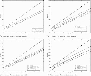
Figure 1. Throughput values as a function of the number of servers when B = 0.
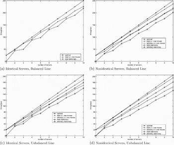
Figure 2. Throughput values as a function of the number of servers when B = 5.
6. COUNTERINTUITIVE EXAMPLES
In this section we provide examples with a dedicated server at each station and also a flexible server to illustrate the fact that both the selection of the downstream, upstream, and flexible servers and the assignment of the dedicated servers to the stations can depend on the buffer size B. Consequently, these examples suggest that obtaining structural results beyond the ones provided in this article that specify the optimal choice of the flexible server and to what stations the dedicated servers should be assigned is difficult.
Consider the case with μ11 = 1.0, μ12 = 1.099, μ21 = 1.1, μ22 = 1.21, μ31 = 3.0, and μ33 = 3.3. If B = 0, then the policy that assigns server 1 to station 1 and server 2 to station 2 and has server 3 as the flexible server is optimal among all the policies with only one flexible server (although the servers are not generalists in this example, this is consistent with Proposition 4.2). The same policy is also optimal for systems with B = ∞. Then one might expect that this policy is also optimal for all 0 < B < ∞. However, this statement is not correct. It turns out that the optimal policy with one flexible server for B = 1 is the one that assigns server 2 to station 1, and server 1 to station 2 and has server 3 as the flexible one. Even though the policy with server 1 at station 1, server 2 at station 2, and server 3 moving is optimal for all B ≥ 6, for B < 6 the optimal policy alternates between the two policies mentioned earlier. Note that the counterintuitive behavior described in this paragraph can also occur when the servers are all generalists. For example, similar results hold for a system with generalist servers where γ1 = 1.0, γ2 = 1.1, μ1 = 1.0, μ2 = 1.1, and μ3 = 3.0.
The examples in the previous paragraph also show that if a policy is optimal for two systems with buffer size B 1 and B 2, respectively, where B 1 < B 2 < ∞, it is not necessarily correct that it is optimal for all B 1 ≤ B ≤ B 2. Moreover, it indicates that even if the optimal choice of which servers are dedicated does not depend on B, the assignment of the dedicated servers to stations might nevertheless depend on the buffer size.
With the next example we demonstrate that the choice of the flexible server can also depend on the buffer size. Suppose that μ11 = 6.0, μ12 = 5.0, μ21 = 4.1, μ22 = 4.01, and μ31 = μ32 = 5.0. For B = 0, the policy that assigns server 1 to station 1 and server 2 to station 2 and has server 3 as the flexible one is optimal. On the other hand, when B = 1, the optimal policy involves assigning server 2 to station 1 and server 3 to station 2 and having server 1 as the flexible server. Finally, when the buffer size is large, the optimal policy assigns server 1 to station 1 and server 3 to station 2 and has server 2 as the flexible one. Hence, depending on the buffer size, the optimal policy with one flexible server can have any one of the three servers as the flexible one.
7. NUMERICAL RESULTS
In this section we provide numerical results for systems with two stations, 1 ≤ M ≤ 10 servers, and exponentially distributed service requirements. Our objective with these numerical experiments is to see the effects of server flexibility on system throughput. Toward this end, we consider systems with a buffer of size B ∈ {0, 5, 10, 20} between the two stations and generalist servers (i.e., μij = μiγj for all i ∈ {1, … , M} and j ∈ {1, 2}). We consider four different sets of numerical experiments for each buffer size B. In the first set of experiments, μi = 50 for all i ∈{1, … , 10} and γ1 = γ2 = 1. In the second set of experiments, the service rate μi of server i ∈ {1, … , M} is drawn independently from a uniform distribution with range [0, 100] and γ1 = γ2 = 1. In the third set of experiments, μi = 50 and γ1 and γ2 are drawn independently from a uniform distribution with range [0, 2]. Finally, in the fourth set of experiments, μi, for i ∈ {1, … , M}, is drawn independently from a uniform distribution with range [0, 100] and γ1 and γ2 are drawn independently from a uniform distribution with range [0, 2]. Note that in all four sets of numerical experiments, the mean of μi, for i = 1, … , M, is 50 and the common mean of γ1 and γ2 is 1, but the variance of μi, for i = 1, … , M, is either zero or 104/12, and, similarly, the common variance of γ1 and γ2 is either zero or 1/3. Hence, the first set of numerical examples is concerned with situations in which the servers are all identical and the line is balanced; the second set focuses on situations with nonidentical servers and balanced lines; the third set addresses situations where servers are all identical and the line is unbalanced; and the fourth set of numerical examples studies situations with nonidentical servers and unbalanced lines.
For all four sets of numerical experiments, we consider five different policies:
• an arbitrary stationary policy where server 1 and all even-numbered servers except for server 2 work at station 1 and the remaining servers work at station 2;
• the best stationary policy (i.e., the policy with the largest throughput among those with l = 0);
• an arbitrary policy with only one flexible server (so that l = 1) assigned optimally to stations, which is any nonidling policy for M = 1, server 1 works at station 1 and server 2 is flexible for M = 2, and for M ≥ 3, server 3 moves, all remaining odd-numbered servers work at station 1, and all even-numbered servers work at station 2;
• the best policy with one flexible server and dedicated servers at both stations when M ≥ 3 and a dedicated server at one station when M = 2 (i.e., the policy with the largest throughput among those with l = 1 and dedicated servers at both stations when M ≥ 3 and a dedicated server optimally assigned to one station when M = 2);
• the optimal policy where all servers are allowed to move (l = M).
For each buffer size B, we compute the long-run average throughput of these five policies when the number of servers M varies from 1 to 10. Clearly, in the first set of experiments, the long-run average throughput of all five policies can be computed exactly. Moreover, in this case, since the throughputs of the arbitrary and best stationary policies are equal to each other and, similarly, the throughputs of the arbitrary and best policies with one flexible server are also equal to each other, we have only three different policies to compare. However, in the remaining three sets of numerical experiments, the long-run average throughputs of the five policies are estimated by finding the average throughput values of 1,000,000 replications for systems with 0 or 5 buffers, 500,000 replications for systems with 10 buffers, and 100,000 replications for systems with 20 buffers and for all choices of M (where each replication involves generating a different set of service rates μij, for i ∈ {1, … , M} and j ∈ {1, 2}, and determining the throughput of the five policies under consideration for these service rates). Figures 1 through 4 display the throughputs of these policies for the four sets of numerical experiments as a function of the number of servers for the four different choices of B.
As expected, Figures 1–4 show that the long-run average throughput of the five policies increases as the number of servers increases. Moreover, the long-run average throughput of the optimal policy is a linear function of the number of servers (as predicted by Theorem 2.1). This assertion seems to hold for the average throughput of the best policy with one flexible server except for the first set of numerical experiments (depicted in plot (a) of Figs. 1–4). Similarly, it holds for the best stationary policy except for the first set of experiments when M > 1 (when M = 1, all policies with l = 0 have throughput equal to zero). Note that since all the servers are identical and the stations are balanced, an additional server does not improve the performance as much in the first set of numerical experiments if it leads to having an unequal number of servers dedicated to stations 1 and 2. Figures 1–4 also demonstrate that one can significantly improve the throughput by allowing servers to move. As Proposition 5.2 suggests, the performance of the best policy with one flexible server approaches that of the optimal policy as the buffer size increases. In fact, even for B = 5, the throughput of the best policy subject to one flexible server is close to the throughput of the optimal policy. Also, in numerical results not presented here in the interest of space, we found that when the optimal policy is considered as the baseline, the difference between the throughputs of the best policy subject to one flexible server and the optimal policy was always less than 17.2% for systems with B = 1 and less than 11.5% for systems with B = 3 (for all four sets of numerical experiments and all 1 ≤ M ≤ 10). This suggests that employing the best policy with one flexible server can yield near-optimal throughput even for systems with small to moderate buffer sizes. On the other hand, even though an arbitrary policy with one flexible server is better than an arbitrary stationary policy, one has to be careful when using an arbitrary policy with only one flexible server. As Figures 2–4 illustrate, the best stationary policy starts outperforming the arbitrary policy with one flexible server as the buffer size and the number of servers increase.
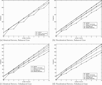
Figure 3. Throughput values as a function of the number of servers when B = 10.
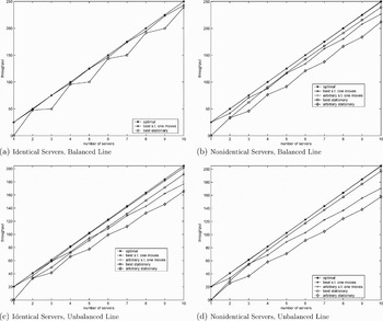
Figure 4. Throughput values as a function of the number of servers when B = 20.
Finally, we comment on the improvement that we obtain by cross-training another server versus the improvement obtained by adding a resource (i.e., a new server or a buffer space). As Figures 1–4 illustrate, in all four sets of numerical experiments, the arbitrary policy with one flexible server among M (for M = 2, … , 9) servers yields very similar throughput as the arbitrary stationary policy with M + 1 servers (considering the arbitrary stationary policy with M + 1 servers as the baseline, the difference between throughputs is less than 6% except when M is odd in the first set of numerical experiments in which case the difference is less than 22%). The same assertion holds when comparing the best policy with one flexible server among M servers with the best stationary policy with M + 1 servers (in this case, the difference between throughputs is at most 24.1% considering the best stationary policy with M + 1 servers as the baseline and this difference decreases as the number of servers increases). This suggests that, on average, increasing flexibility is almost as effective as increasing the number of servers in terms of improving throughput.
On the other hand, having all the servers flexible and assigning them optimally to the stations is more effective than adding buffer space. This is consistent with Theorem 2.1, which shows that when the servers are generalists, the optimal throughput (under the assumption that all servers are flexible) does not depend on the buffer size. Hence, for a fixed number of servers M, the throughput of the optimal policy for systems with B = 0 is larger than the throughput of all other policies for systems with B > 0. Similarly, in plots (b), (c), and (d) in Figures 1–4, for all M = 1, … ,10, the throughput of the best policy with one flexible server for systems with B = 5 outperforms the throughput of the best stationary policy for systems with B = 10 and the throughput of the best policy with one flexible server for systems with B = 10 outperforms the throughput of the best stationary policy for systems with B = 20. The same assertion holds for plot (a) (the first set of numerical experiments) when the number of servers is odd. When the number of servers is even, the throughput performance of the two policies for the corresponding systems is very similar (the throughput for the systems with one flexible server and the smaller buffer size is slightly smaller). Even though the throughput of the best policy with one flexible server for systems with B = 0 is, in general, less than the throughput of the best stationary policy for systems with B = 5, the difference between the throughputs is small in most cases. These observations suggest that, in general, it is more effective to add server flexibility rather than buffer space in order to increase the long-run average throughput.
8. CONCLUSIONS
For a tandem queuing network with N ≥ 2 stations, M ≥ 1 servers, an infinite supply of jobs in front of station 1, infinite room for completed jobs after station N, and either a finite or infinite buffer between consecutive stations, we studied the dynamic allocation of servers to stations with the goal of maximizing the long-run average throughput under the assumption that only a subset of the servers are flexible, with the remaining servers being dedicated to particular stations. When N = M = 2 and both servers are dedicated, we have specified which server should be assigned to which station in order to maximize the throughput. When N = 2, 1 ≤ M ≤ 3, and only a subset of the servers are flexible, we have shown that the allocation of the flexible servers is of threshold type and characterized the threshold values. However, the optimal selection of the dedicated and flexible servers, assignment of dedicated servers to stations, and the threshold(s) where the flexible server(s) switch from station 1 to station 2 can depend on the buffer size.
When the servers are generalists, we were able to completely characterize the optimal policy in almost all cases. In particular, when all servers are flexible, we proved that any nonidling policy is optimal for systems with finite buffers. When N = 2, B < ∞, service requirements are exponentially distributed, and all servers are assigned to two dedicated teams, we have shown that it is optimal to assign the faster team of servers to the slower station. Similarly, when N = 2, B < ∞, and the service requirements are exponentially distributed, we proved that the optimal policy should have the fastest l servers as the flexible ones if all of the dedicated servers are at the same station or if there is at least one dedicated server at each station and a single team of flexible servers and also that when all the dedicated servers are at the same station, they should be assigned to the slower station.
Finally, we showed that the throughput of the optimal policy for two-station Markovian tandem queues with M = 2 or M = 3 servers converges to the throughput of the optimal policy for the corresponding infinite-buffered systems as the buffer size becomes large. Moreover, we proved that for large buffer sizes, the throughput of the best policy with a single flexible server for these systems is close to the throughput of the optimal policy where all servers are flexible. Our numerical examples indicated that this assertion also holds for two-station tandem queues with M > 3 servers and moderate buffer size B when the servers are generalists with exponentially distributed service requirements. Furthermore, the numerical results illustrated that, in general, adding flexibility is almost as effective as adding a new server and more effective than adding a buffer space in improving the system throughput.
Acknowledgments
The research of the first author was supported by the National Science Foundation under grants DMI–0000135, DMI–0217860, and DMI–0400260. The research of the second author was supported by the National Science Foundation under grant DMI–9984352. The research of the third author was supported by the National Science Foundation under grant DMI–0000135 and by the Natural Sciences and Engineering Research Council of Canada.
APPENDIX
Proof of Lemma 4.1
If Assumption E holds and π ∈ Π, then it is clear that the stochastic process {X π(t) : t ≥ 0} defined in Section 2.2 is a continuous-time Markov chain and that there exists a scalar q π ≤ ∑i=1Mmax1≤j≤2μij < ∞ such that the transition rates {q π(x, x′)} of {X π(t)} satisfy ∑x′∈S,x≠x′q π(x, x′) ≤ q π for all x ∈ S. Hence, {X π(t)} is uniformizable for all π ∈ Π. Let {Y π(k)} be the corresponding discrete-time Markov chain, so that {Y π(k)} has state space S and transition probabilities p π(x, x′) = q π(x, x′)/q π if x ≠ x′ and p π(x, x) = 1 − ∑x′∈S,x≠x′q π(x, x′)/q π for all x ∈ S. It has been shown by Andradóttir et al. [Reference Andradóttir, Ayhan and Down6] that the original optimization problem in (1) can be translated into an equivalent (discrete-time) Markov decision problem. More specifically, let
be the departure rate from state x under policy π, for all x ∈ S and π ∈ Π. Then the optimization problem (1) has the same solution as the Markov decision problem
![$$\mathop{\max}\limits_{\pi \in \Pi} \lim_{K \rightarrow \infty } {\open E} \left[{1 \over K} \sum\limits_{k = 1}^{K} R_{\,\pi} \lpar Y_{\,\pi} \lpar k - 1\rpar \rpar \right].$$](https://static.cambridge.org/binary/version/id/urn:cambridge.org:id:binary:20151022132024594-0921:S0269964807000290_eqnA1.gif?pub-status=live)
In what follows, we solve a more general problem that determines the optimal allocation of servers 2 and 3 subject to having at least one server at station 2 at all times (but this server could depend on the state) and server 1 at station 1 at all times. Since (as we show below) the optimal policy for this less restrictive problem has server 2 dedicated to station 2, server 1 dedicated to station 1, and server 3 flexible, we can conclude that the faster server should be the flexible one when there is a dedicated server at each station.
It follows from Proposition 2.1 of Andradóttir and Ayhan [Reference Andradóttir and Ayhan5] that it is sufficient to consider actions that do not allow the flexible servers to idle. Then the set As of allowable actions in state s ∈ S is given by A s = {d 0, d 1, d 2} for s ∈ {0, … , B + 1} and A B+2 = {d 1}, where
From our assumptions on the service rates, we have a recurrent Markov decision process and we can use the policy iteration algorithm for unichain models (see Puterman [Reference Puterman25, p. 378]) to prove the optimality of the policy described in Lemma 4.1.
In the policy iteration algorithm, we start by choosing
corresponding to the policy described in Proposition 4.1. Then the reward vector r δ0 and the probability transition matrix Pδ0 corresponding to the decision rule δ0 are given as
and
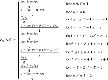
Since the Markov chain under the policy (δ0)∞ is irreducible, we can find a scalar g 0 and a vector h 0 solving
subject to h 0(0) = 0. In (A2), e is a column vector of ones and I is the identity matrix. Define
and
One can show that g 0 = Φ0/Φ1, h 0(0) = 0,

for 1 ≤ s ≤ s*, and
for s* + 1 ≤ s ≤ B + 2, constitute a solution to (A2). As is discussed in Puterman [Reference Puterman25, pp. 338–339], g 0 represents the long-run average reward under policy (δ0)∞ (which is the long-run average throughput under policy (δ0)∞) and h 0(s), s = 1, … , B + 2, can be interpreted as the asymptotic relative difference in total reward that results from starting the process in state s versus state 0.
As the next step of the policy iteration algorithm, we choose
setting δ1(s) = δ0(s) if possible (here r(s, a) is the reward gained when action a is chosen in state s and p(j|s, a) is the transition probability from state s to state j when action a is chosen in state s). We now show that if s* ∈ S*, then δ1(s) = δ0(s), for all s ∈ S. In particular, for all s ∈ S and a ∈ A s, we will show that the differences
are nonpositive. Thus, we will prove that the decision rule corresponding to (δ0)∞ (which is the policy described in Lemma 4.1) satisfies the optimality equations and, hence, it is gain (long-run average reward) optimal.
For 0 ≤ s ≤ s* − 1, we have that δ0(s) = d 0. Define
We have
and
Similarly, for s* ≤ s ≤ B + 1, we have that δ0(s) = d 1. Define
We have
and

Since A B+2 = {d 1}, we have shown that δ1(s) = δ0(s) for all s ∈ S. By Theorem 8.6.2 of Puterman [Reference Puterman25], this proves that the policy described in Lemma 4.1 is optimal.■


