


I. INTRODUCTION
Many geologists, regardless of their scope of scientific interests, face the problem of comparing mineralogical and geochemical data. In most cases, this comparison is nearly intuitive and limited to a simple collation of the geochemical data and results of separately obtained mineralogical studies. When selecting geochemical samples, geologists exert every effort to make their collections as representative as possible. To that end, they practice a diversity of specific sampling techniques, whose purpose is to characterize a significant rock volume. In mineralogical investigations, on the contrary, local methods (electron microprobe analysis, LA-ICP-MS, etc.) dominate, and most of the used preparations (thin sections, polished sections, etc.) have only two-dimensional sections of sub-inch areas of a sample. Thus, a researcher deals with a comparison of differently scaled objects, i.e. geochemical data characterizes a significant rock volume, while mineralogical data describes its parameters in a limited piece only. Nevertheless, the latter is usually extrapolated to the same volume of matter that geochemical information was obtained for. Such an extrapolation is incorrect, primarily for rocks with taxitic structure. This includes all kinds of metasomatites, as well as many magmatic and metamorphic formations. The methodology we propose helps to compare mineralogical and geochemical data obtained for the same volume of matter, i.e. single-scaled matter.
Second, the problem is that the traditional approach to comparing geochemical and mineralogical data is close to “intuitive”. Since the information to be analyzed is complex, this approach allows us to identify only the most vivid links. Such a comparison is challenging even for a small collection. However, representative sample set a priori must be large. Methods of statistical data analysis have long been applied to searching complex dependencies in geology (Jöreskog et al., Reference Jöreskog, Klovan and Reyment1976; Swan and Sandilands, Reference Swan and Sandilands1995; Davis, Reference Davis2002). The most important aspects of their application are the decreased impact of an experimenter's subjective view and the possibility of assessing the value of the revealed dependencies. However, investigations with statistically compared mineralogy and geochemistry are scarce. The development of this study area with classical petrographic–mineralogical methods is constrained by a very time-consuming process of collecting a necessary amount of mineralogical information. For example, the paper (Xie et al., Reference Xie, Last, Murray and Mackley2003) highlights one of the few examples of a thorough statistical comparison of geochemistry and mineralogy, but it took more than 30 years to compile the primary database.
In our approach, the X-ray diffraction patterns of the bulk samples (the same powders as used for chemical analyses) were used to reveal the mineral composition of the rock. Considering the current level of analytical techniques, these data are quickly obtained, even if samplings are vast. The main problem of determining both qualitative and (especially) quantitative mineral composition by classical methods is that it is based on work with individual spectra, which is a laborious task. Traditional standardless quantitative methods usually include sophisticated structure refinement procedures (e.g., Rietveld refinement). Methods involving an internal standard are not optimal for compact analysis and are often prone to prediction errors caused by the intensity attenuation (Moore et al., Reference Moore, Cogdill and Wildfong2009). Moreover, they require a priori information about the set of components. An effective solution to this problem is to apply the statistical methods of blind signal separation (i.e. the separation of a set of source signals from a set of mixed signals, without the aid of information about the source signals or the mixing process), widely used in the study of various spectral data obtained by X-ray powder diffraction (XRPD), Raman spectroscopy, energy dispersive X-ray fluorescence (EDXRF) spectrometry, and X-ray absorption spectroscopy (XAS). For blind signal separation in spectral data, factor analysis (FA) in the modification of principal component analysis (PCA), singular value decomposition (SVD), a multidimensional regression method, multivariate curve resolution (MCR), and other related methods are most often used. These methods serve to solve a wide range of tasks, e.g.: (1) analyzing large (thousands of spectra) datasets and increasing the efficiency of data collection (Kirian et al., Reference Kirian, White, Holton, Chapman, Fromme, Barty, Lomb, Aquila, Maia, Martin, Fromme, Wang, Hunter, Schmidt and Spence2011; Angeyo et al., Reference Angeyo, Gari, Mangala and Mustapha2012; Voronov et al., Reference Voronov, Urakawa, van Beek, Tsakoumis, Emerich and Rønning2014; Palin et al., Reference Palin, Caliandro, Viterbo and Milanesio2015; Guccione et al., Reference Guccione, Palin, Belviso, Milanesio and Caliandro2018); (2) determining the relations between developments in XRD data and other systematically changing properties (strength, viscosity, and volume) (Westphal et al., Reference Westphal, Bier, Takahashi and Wahab2015); (3) estimating the number of phases in the system and identifying each phase (Artyushkova and Fulghum, Reference Artyushkova and Fulghum2001; Caliandro et al., Reference Caliandro, Di Profio and Nicolotti2013; Manceau et al., Reference Manceau, Marcus and Lenoir2014); (4) reducing the influence of the signal-to-noise ratio (Sastry, Reference Sastry1997; Schmidt et al., Reference Schmidt, Rajagopal, Ren and Moffat2003; Chen et al., Reference Chen, Morris, Martin, Hammond, Lai, Ma, Purba, Roberts and Bytheway2005; Walton and Fairley, Reference Walton and Fairley2005); (5) investigating the orientation and morphology of crystalline phases (Matos et al., Reference Matos, Xavier, Barreto, Costa and Gimenez2007); (6) tracking the development of complex processes of compositional and structural alterations in a multicomponent system (Westphal et al., Reference Westphal, Bier, Takahashi and Wahab2015); (7) performing the analysis of time-resolved experimental data (Schmidt et al., Reference Schmidt, Rajagopal, Ren and Moffat2003; Mabied et al., Reference Mabied, Nozawa, Hoshino, Tomita, Sato and Adachi2014); (8) extracting kinetic information (the activation energy, the frequency factor, the reaction order, etc.) (Palin et al., Reference Palin, Conterosito, Caliandro, Boccaleri, Croce, Kumar, van Beek and Milanesio2016; Guccione et al., Reference Guccione, Palin, Belviso, Milanesio and Caliandro2018). In our study, the solution of (1)–(3) tasks from the above list is discussed, and the chemical composition of rocks is considered as systematically changing properties.
This paper presents a version of the statistical comparison of geochemical information with the mineralogical data contained in the XRD-patterns using the “blind” application of factor analysis in PCA modification. Importantly, it does not require the time-consuming step of quantitative determination of the mineral composition. Since methods of statistical processing in widely available software packages (SPSS, Statistica, etc.) are also simple, our method provides an express statistical comparison of geochemical and mineralogical data at the earliest stages of research. The size of the sample set influences the effectiveness of the method, and the signal-to-noise ratio is not critical. If sampling is large (of more than 40 samples), factor analysis allows us to identify the entire set of main rock-forming, secondary and some accessory minerals in the rocks.
II. ANALYSIS OF EXPERIMENTAL DATA
A. Research material and analytical methods
We investigated sample collections of two geological objects of the Kola region (northwest Russia): 43 samples of rare-earth carbonatites of the Petyayan–Vara field (the Vuoriyarvi Devonian alkaline-ultrabasic carbonatite massif) and 19 samples of the sillimanite schists of the Makzabak mountain (contact rocks of the Keivy Precambrian supracrustal complex near alkaline granites of the Western Keivy massif). With all the differences, all these rocks have a pronounced taxitic structure and formation during several superimposed metasomatic events (Kozlov et al., Reference Kozlov, Fomina, Sidorov and Shilovskikh2018; Fomina et al., Reference Fomina, Kozlov, Lokhov, Lokhova and Bocharov2019). In this regard, the identification of the relationship of a chemical element distribution with a specific mineral association is an important task. Samples of each collection are mixtures of more than ten minerals of variable quantities.
The principal sample set for this research was the collection of the Petyayan–Vara carbonatites, which is larger and more widely studied both geochemically and by RFA. The X-ray powder diffraction data of the bulk carbonatite samples were collected at room temperature by the Rigaku MiniFlex II diffractometer, using a Cu target X-ray generator operated at voltage 30 kV and current 15 mA. The scan range of the Bragg angle (2θ) was from 3.00° to 70.00° with a step width of 0.02° and a counting time of 2 s per step. The obtained “raw” spectra are listed in the Electronic Supplement (Table S1).
Since one of the research tasks was to determine the applicability limits of the method, the diffractograms for samples of sillimanite schists were collected less thoroughly. The X-ray powder diffraction data of the bulk sillimanite samples were collected at room temperature by the ARL X'TRA diffractometer, using a Cu anode with Ni filter (Cu Kα = 1.54 Å). The scan range of the Bragg angle (2θ) was from 5.00° to 75.00° with a step with of 0.02° and a counting time of 2 s per step. Nickel filter was used to eliminate the CuKβ radiation due to the using a goniometer without a monochromator. This leads to an overestimated background. As a result, even visually it is noticeable that these diffractograms have a significantly higher noise-to-signal ratio (Figure 1).

Figure 1. The examples of raw diffractograms of the “good” and “poor” data sets (collections of the Petyayan–Vara carbonatites and the Makzabak sillimanite schists, respectively).
The purpose of the method was to compare the geochemical and mineralogical characteristics of the rocks; therefore, we made chemical analyses of the samples of both collections. The contents of petrogenic and volatile components were studied with classical methods of “wet” chemistry at the GI KSC RAS. Analyzing concentrations of SiO2, Al2O3, Fe2O3, MgO, TiO2, SrO, average portions of the matter were decomposed by melting with borax and soda, and then transferred into the solution. A separate sample, also melted with borax and soda, was used to determine the F content, while Cl was analyzed after sintering with KNaCO3. In addition, certain samples were decomposed by acid in the mixture (H2SO4 + HNO3 + HF) to analyze concentrations of K2O, Na2O and MnO; in the mixture (HNO3 + HF) to analyze P2O5; in a mixture (H2SO4 + HF) to analyze FeO; and in nitric acid to calculate the S content. To analyze CO2 content, the tested powder was previously exposed to NaOH. Analyses of SiO2, Al2O3, Fe2O3, MgO, CaO, SrO were carried out by the atomic absorption method; those of K2O, Na2O, MnO with the emission method; TiO2, P2O5 with the colorimetric method; F, Cl with direct potentiometric determination; CO2, FeO with titration; and Stot, H2O+ and H2O– gravimetrically. The measurement error limits were 1.5% for concentrations >10 wt.% and 3.5% for concentrations >1 wt.%.
Additionally, we analyzed the concentrations of trace elements in the Petyayan–Vara carbonatites. They were determined by inductively coupled plasma emission mass spectrometry (ICP-MS) on the ELAN 9000 DRC-e quadrupole mass spectrometer (ICTREMRM KSC RAS). In this case, a sample was transferred completely into the solution after acid decomposition in glassy carbon crucibles, gradually adding distilled HF (triple addition and evaporation to wet salts) and HNO3. The resulting sample solutions were diluted in such a way that the intensities of the analytical signals corresponded to the selected calibration ranges. The precision of the ICP-MS measurement is better than ±15% for most of elements. The Electronic Supplement provides the measured contents of major and trace elements in the Petyayan–Vara carbonatites (Table S2).
Thus, to test the proposed method, we used two sets of data that differed significantly in their geological information quality (number of samples, quality of diffractograms, completeness of the geochemical characteristics): “good” data for the Petyayan–Vara carbonatites and “poor” data for the Makzabak sillimanite schists.
B. Theory and calculation
As noted above, X-ray diffraction patterns served as a source of mineralogical information on bulk rock samples in the suggested method. This is based on the following set of diffractograms properties:
• The powder diffraction pattern is an individual characteristic of a crystalline substance;
• Each crystalline phase always displays the same diffraction spectrum characterized by a specific set of interplanar distances d(hkl), which can also be represented in the values of the 2θ angle, and the corresponding line intensities I(hkl), unique to this crystalline phase;
• The X-ray diffraction spectrum of a mixture of individual phases is a superposition of their diffraction spectra;
• The ratio of the intensities of crystalline phases present in a sample is proportional to the content of the phases in it.
These properties are the basis of qualitative and quantitative methods of X-ray phase analysis (Klug and Alexander, Reference Klug and Alexander1974; Jenkins and Snyder, Reference Jenkins and Snyder1996). In our case, it is also important that intensities of individual peaks of each mineral are proportional to each other and thus correlated. This allowed the use of the factor analysis (FA) as a separator to sort data regarding different mineral phases “hidden” in diffractograms, since it focuses on emphasizing components of correlated data.
FA is aimed at ascribing a large and unwieldy set of original (measured) variables to a smaller set of latent variables called factors. In the actual study, FA was applied to minimize the number of variables (factors) necessary to represent all non-random differences in a united dataset of diffractograms and chemical analyses of rock samples without losing significant information. For this purpose, the principal component analysis (PCA) was used. As a rule, FA is performed in two steps: determining the factors and interpreting the factor meanings. An FA is successful only if an interpretation can be found for the factors.
Mathematically, the procedure for factor extracting can be described as follows. Suppose we have a matrix of X variables of (N × M) size, where N is the number of samples (rows) and M is the number of independent variables (columns, in the present study, 2θ values for XRPD + element contents), which are usually numerous (M ≫ 1). The analysis can be carried out by examining either the correlation matrix, or the covariance matrix for variables (R-technique), or the observations (Q-technique) of the X matrix. Most often, the correlation matrix for variables is examined, which requires additional data processing (Jolliffe, Reference Jolliffe2002). The X matrix must be converted to a standardized XS matrix. For this, each x ij value is replaced by a standardized value calculated by the formula
 $$x_{ij}^S = \displaystyle{{x_{ij}-{\bar{x}}_j} \over {\sigma _j}},$$
where  $\bar{x}_j$ is the mean and σ j is the standard deviation.
The standardized data matrix is decomposed into a number of latent variables (factors) that maximize the explained variance in the data on each successive factor, under the constraint of being orthogonal to the previous factor. They are calculated as eigenvectors of the correlation matrix of the standardized data, and the magnitude of the corresponding eigenvalues represents the variance of the data along the eigenvector directions (Wold et al., Reference Wold, Esbensen and Geladi1987). The initial dimensionality of the dataset, equal to the number of columns (N), is reduced n, representing the number of the used factors. The optimal value of n can be determined by considering the sum of the eigenvalues of the used factors, which represents the data variability explained by the chosen factors.
Decomposition of an XS data matrix is an operation of data separation into a structure part and a noise part:
 $${\bf X}^S = {\bf T}{\bf P}^T + {\bf E} = {\rm Structure} + {\rm Noise},$$
where T is the matrix of scores, of size N × n, P is the matrix of loadings, of size M × n, apex T means transpose, and n ⩽min (N,M) (N is the number of samples, M is the number of independent variables, n is the number of factors). The residuals (noises) are collected in an E matrix such a way that T describes the position of the samples in the new coordinate system. P describes the new axis, which is built on the original one. The score values describe the magnitude of a factor. The loadings are basically the correlation coefficients between the factors and the original variables. Statistical significance of the loadings can be estimated using standard tests. In the actual study, for the sample set of the Petyayan–Vara carbonatites (43 samples), the factor loading (hereafter, r FA) critical value module is 0.30 at a significance level of p = 0.05, and 0.48 at a significance level of p = 0.001 (correlation is insignificant at r FA <|r FAcrit.|). For the sample set of the Makzabak sillimanite schists (19 samples), the corresponding values are 0.46 and 0.69, respectively.
In the decomposition step, the scores and loadings are sorted according to the fraction of the total data variance they are able to explain. To interprete the results is to decipher the information hidden in the parameters of the scores and/or the loadings. To simplify the interpretation of results, the procedure of orthogonal or oblique rotation of factors is commonly used at the final stage. Its task is to achieve the so-called “simple structure”. The structure is considered simple, if only some of the loadings of each rotated factor are big, while the others are close to zero. A rotation serves to represent each original variable by only a few (ideally, by one) factors. VARIMAX rotation (Kaiser, Reference Kaiser1958), which is the most commonly used orthogonal rotation in factor analysis (Izenman, Reference Izenman2008), was applied. Starting with the first factor, each factor is consecutively rotated to maximize the data variance explained by this factor. Further details of FA and PCA can be found elsewhere (e.g., Jöreskog et al., Reference Jöreskog, Klovan and Reyment1976; Wold et al., Reference Wold, Esbensen and Geladi1987; Jolliffe, Reference Jolliffe2002).
A demonstrative example of how FA (PCA) results are interpreted is the solution of the common mineralogical problem of determining isomorphism mechanisms. Variations in the chemical composition of minerals are conditioned by the occurrence of various elements in the same structural position(s). The elements are strictly limited to the possible structural positions of the crystal lattice. They compete for these positions and can enter the crystal structure either individually or in groups, with the condition that the charge element is retained. One element can simultaneously participate in several isomorphic substitutions. For minerals of complex composition (with several structural positions), the discussed problem is nontrivial. The effectiveness of the use of FA is determined by the presence of “either-or” combinations (due to the competition of elements) and “and-and” combinations (occupation the position of one group of elements by either another group or one element with the formation of a vacancy to preserve the total charge). Since isomorphism is responsible for variations in the chemical composition of minerals, the application of FA to sets of chemical compositions of minerals reveals information about this phenomenon. There, the isomorphic substitution reactions are reflected in factors. The values of the factor loadings indicate in which reaction(s) a certain element participates. Elements connected by “and-and” type are grouped due to high loadings of the same sign (negative or positive). The “either-or” connection is realized by separating competitors with factor loadings of different signs. Factor values indicate the significance of each identified isomorphism type in a particular analysis. Thus, FA is effective even in the study of minerals with complex chemical composition and structure (e.g., Selivanova et al., Reference Selivanova, Lyalina and Savchenko2018).
This example shows the importance of the initial understanding of the causes of variability of the studied properties (variables) for the quality of interpretation. In the actual study, using the factor analysis, the intensities for the XRPD-patterns and the contents of elements were studied. Variations of all variables describing these properties are determined by variations in the mineral content of the studied rocks. The factors correspond to those parts of the total dataset which belong to particular minerals, if the changes in their content in the rocks are correlated. Hence, the values of factor loadings indicate which parts of the rock spectrum contain the lines of a particular mineral and which elements are concentrated in this mineral. Also, it displays the contribution of the latter to the distribution of these elements in rocks. Factor scores in this study are the numerical expressions of the mineral(s) contents in each analysis.
We present the calculation algorithm on the example of the Petyayan–Vara rare-earth carbonatites (“good” data). Preliminary processing of the “raw” X-ray data for factor analysis was done by fitting the graphs to baseline using the CSM-3 software v.3.1.0.2 (Oxford Cryosystems). Transformed in this way, the diffractogram represents an array of numbers, wherein each variable (the value of 2θ angle) corresponds to a certain intensity value. Since spectra were taken in the range of 2θ from 3° to 70° at intervals 0.02°, each diffraction pattern was described by 3351 variables (hereafter, XRD-variables).
Prior to factor analysis, two procedures are required to solve the problem of the analysis of data with equal and/or zero variances (Jolliffe, Reference Jolliffe2002):
(1) The removal of variables, whose values became zero in all diffractograms after fitting to the baseline;
(2) Adding any constant (for example, 1) to each intensity value.
The X-ray data table based on the results of all the above procedures, performed using Excel, is given in the Electronic Supplement (Table S3).
Each sample, in addition to the X-ray data (3351 variables), was characterized by the contents of major and trace elements (47 more variables; hereafter, geochemical variables). Since geochemical variables amount to about 1% of the overall primary data, they did not have any noticeable effect on the extracted factors structure. This was verified by the following numerical experiment. The loading graphs of factors extracted exclusively from data on diffraction patterns are similar to the loading factors extracted from the combined diffraction and geochemical data. Nevertheless, this method allows for the relating of originally “mineralogical” factors to the geochemistry of rocks.
The factors were calculated using generalized data (Table S4) in the IBM SPSS Statistics v.23 software package. The R- technique FA (“on variables”) was applied according to the tasks assigned. Therefore, for the calculations, the matrix of r coefficients between all pairs of “pre-prepared” variables served as a basis. To extract the factors, the principal component analysis was used. The factors with eigenvalues exceeding 1 were extracted and rotated with the VARIMAX technique. The factor values were defined using the regression analysis. All these steps are included in the standard settings of the program. This allows the configuration of the analysis in a matter of minutes regardless of one's mathematical competence and experience of work with IBM SPSS Statistics, if any. At this stage, obstacles may appear only due to the lack of rotation convergence. This can be solved by increasing the number of iterations (in our case, it took 107). Supplementary Table S5 provides results of the calculations (factor loadings, r FA).
C. Results
According to the results of factor analysis of the Petyayan-Vara sample collection (“good” data), only 14 factors had any statistically significant influence on the distribution of major (Table I) and most trace elements (Table II). Therefore, only these 14 factors were studied. Based on factor scores and factor loadings on XRD-variables and geochemical variables, these factors are determined by variations in the contents of the following minerals (in order of their dispersion decrease being explained by factors): baryte, dolomite, calcite, ancylite-(Ce), microcline, phlogopite, fluorapatite, quartz, strontianite, goethite, albite, aegirine, hydroxylbastnäsite-(Ce), and ankerite (Figure 2).
Table I. Factor loadings (r FA) of major components on factors significantly related to the distribution of elements in the rocks.

Here and in Table II statistically significant loadings are bold.
a In Tables I, II, as well as in Figure 2 factors are indicated by abbreviations of the corresponding minerals: Brt, baryte; Dol, dolomite; Cal, calcite; Anc, ancylite-(Ce); Mc, microcline; Phl, phlogopite; Ap, fluorapatite; Qz, quartz; Str, strontianite; Gth, goethite; Ab, albite; Aeg, aegirine; Bas, hydroxylbastnäsite-(Ce); and Ank, ankerite.
Table II. Factor loadings (r FA) of trace elements on the factors under consideration.

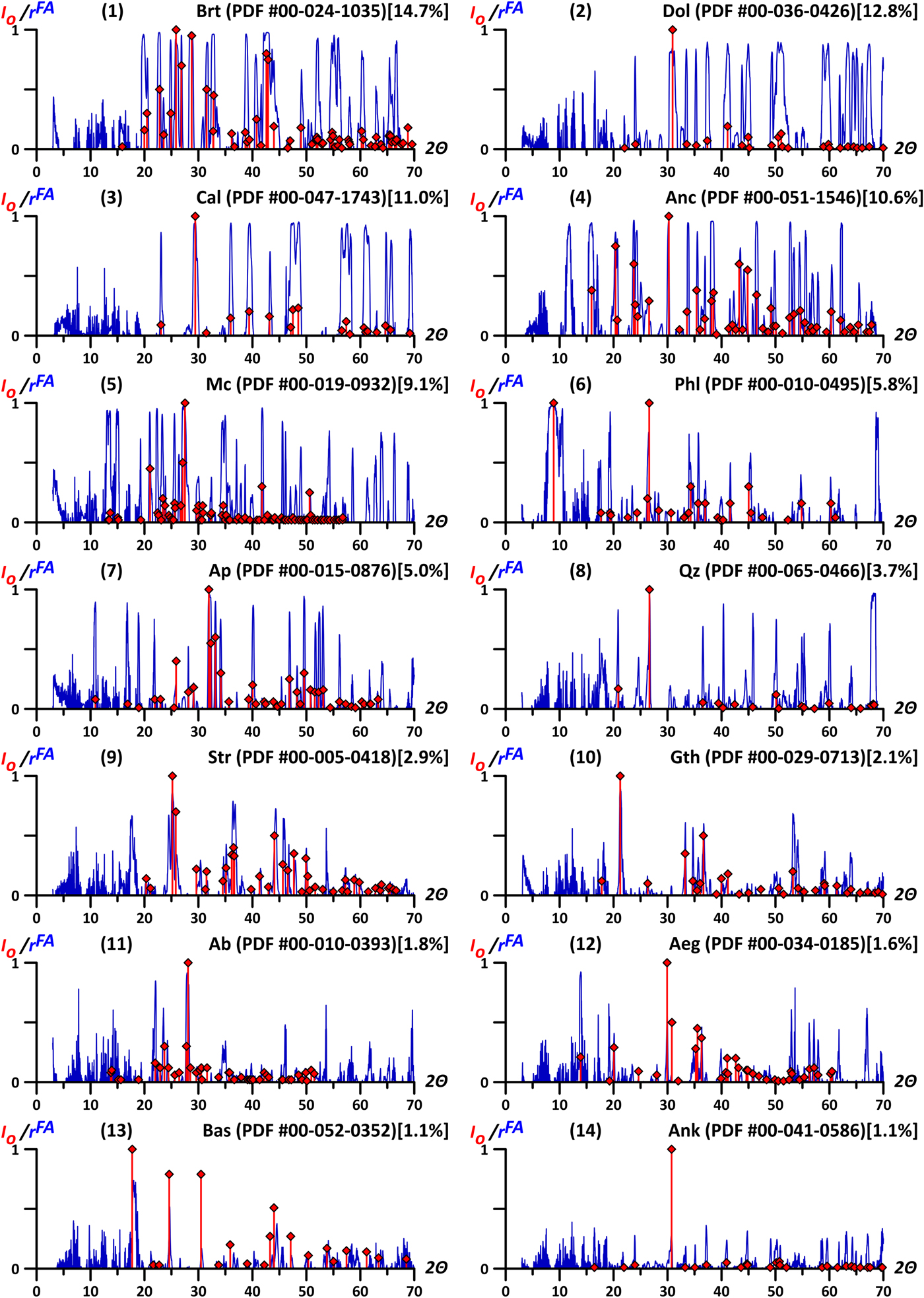
Figure 2. (Colour online) The comparison of factor loading values (r FA) of the detected factors (blue lines) with peak positions in the diffractograms corresponding to the mineral factors (red bars, I O – relative intensities, the largest peak value is 1). The r FA graphs are given in the descending order of dispersion explained by a factor (the fraction of the latter is provided in square brackets). Diffraction patterns of the minerals are taken from the ICDD PDF-2 database, the corresponding PDF-cards numbers are in parentheses. Since all negative factor loadings are greater than critical value of −0.30 (p = 0.05), they are excluded for simplicity.
The above list of phases almost entirely corresponds to the set of main rock-forming and secondary minerals in the samples of the Petyayan–Vara collection. Factor scores reflect the content of these minerals in the samples. This is evident when comparing the content of barium and factor scores of the baryte factor (baryte is the only host of Ba in the studied rocks) (Figure 3). In all cases, the maximum values of the factor scores accurately indicate the samples richest in the mineral to which this factor corresponds.

Figure 3. (Colour online) Binary diagram “content of barium” (Ba, wt%) vs “factor scores of the baryte factor” (Score).
Factor loadings on XRD-variables are clearly similar to the X-ray spectra of corresponding minerals from specialized XRPD databases. For this study, ICDD PDF-2 database was used. For comparison, preferably the patterns with star quality marks (well characterized chemically and crystallographically, with no unindexed lines and Δ2θ ⩽0.03°) were chosen. The similarity of factor loadings and the X-ray spectra is clearly illustrated with an example of the fluorapatite factor (Figure 4) corresponding to the spectrum (7) on Figure 2. A comparison of the graphs of factor loadings values (r FA) and the X-ray pictures of minerals revealed almost an absolute coincidence of peak positions (the peaks positions on the r FA graphs almost always differ from those on the diffractograms of standards by no more than ±0.1°). However, the intensities of these peaks are not equal. Based on data analysis, we found the peak heights on the graphs of factor loading values do not only depend on the intensities of the corresponding mineral reflexes (Figure 5). The diagrams show that the positions of the most intense peaks of standards correspond to the highest values of factor loadings. Nevertheless, weak peaks are sometimes expressed in comparable r FA values, although there are no r FA peaks near the position of many small peaks of the standards. The intensity lines of other minerals adjacent to the considered reflexes appeared to obscure peaks heights, thus reducing the values of factor loadings. For the same reason, the graphs of factor loadings of apatite and other listed minerals have unexpectedly high peaks from rather weak mineral lines in segments of the spectrum free from extraneous reflexes. The listed properties are well-observed in the remaining 13 graphs of the considered factors. Taking this into account, we identified the mineral phases corresponding to each factor by searching them in X-ray databases, focusing specifically on the peak positions of the factor loadings.

Figure 4. (Colour online) The comparison of the fluorapatite X-ray diffractogram from the RRUFF database (analysis R050529, red line; I O – relative intensities, the largest peak value is 1) with the factor loading values (r FA) of the detected apatite factor (blue line) for the 2θ-values ranging from 10° to 70°. Since all negative factor loadings are greater than critical value of −0.30 (p = 0.05), they are excluded for simplicity.

Figure 5. (Colour online) Binary diagrams of “peak intensities in the standard” (I O) vs “factor loading values in 2θ angles of these peaks” (r FA) for the factors of (a) dolomite, (b) calcite, (c) baryte, and (d) apatite. Red circles denote the presence of r FA peak in the range of ± 0.1° from the peak of a standards, blue squares denote its absence. Diffraction patterns of the standards are taken from the ICDD PDF-2 database, the corresponding PDF-cards numbers are in parentheses.
As per the conditions of the factor extraction, each of them possesses significant loadings of one or several geochemical variables, often reaching values of 0.8 or more. Hereafter, such elements will be called “indicator elements”. These elements are either in the crystallochemical formula of the corresponding mineral, or its typical impurities. The examples are barium (0.92) and sulfur (0.93) loadings on baryte factor, or lithium (0.96) on phlogopite factor. On the one hand, these high loadings make it easier to identify a mineral corresponding to a factor. On the other hand, concentrations of these elements are also geochemical markers, allowing a rough estimation of a mineral content in the rock, as confirmed by the petrographic research. For example, there is no phlogopite in the samples from carbonatites with an Li content less than 10 ppm. Vice versa, in rocks containing more than 10 ppm Li, the phlogopite amount increases proportionally to the lithium concentration and reaches its maximum in the sample most rich in Li (450 ppm).
However, the above does not explain high loadings of zirconium (0.82) and hafnium (0.67) on the apatite factor, as well as titanium (0.75), niobium (0.48) and tantalum (0.51) on the microcline and several other factors. In addition, the minerals of titanium, zirconium or niobium are not expressed in the relevant individual factors, although, e.g., titanium oxides are rock-forming in some samples.
In combination, the results obtained for the “good” data proved the fact that the extracted factors are directly related to the mineral composition of the rocks. Thus, our approach is deprived of the main weak spot of factor analysis, i.e., the challenging interpretation of obtained results.
The statistical analysis of “poor” data is much more difficult to interpret. Only the first six of the 18 r FA graphs have clearly distinguishable peaks. Moreover, only two factors are marked by significant loadings on geochemical variables. The morphology of the factor loading graphs differs from that considered earlier. First, the graphs are “noisy”, which, apparently, reflects the high noise-to-signal ratio of the primary data. The r FA graphs of the “good” sampling have the same “noisy” character in the range of 2θ from 3° to 20°, i.e. in the area almost devoid of intense peaks and, as a consequence, with a high “noise-to-signal” ratio as well. Second, these graphs have both positive and negative peaks of r FA. Both have an equally clear mineralogical interpretation. Thus, on the graph in Figure 6, the peaks in the positive region of r FA fully correspond to the peaks of the sillimanite diffractogram. The peaks in the negative region correspond to the staurolite peaks.

Figure 6. (Colour online) The comparison of peak positions in the diffractograms of sillimanite (Winter and Ghose, Reference Winter and Ghose1979) and staurolite (Smith, Reference Smith1968) [red bars and green bars, respectively; I O – relative intensities, the largest peak value is 1] with the factor loading values (r FA) of the detected “sillimanite–staurolite” factor (blue line) for the 2θ-values ranging from 10° to 70°.
The loadings on the geochemical variables obtained during the analysis of “poor” data are as natural as in the case of “good” data. Thus, for the “sillimanite–staurolite” factor in the positive region (the sillimanite component of the factor), the values of r FA on Al (0.63) and Si (0.90) are high. The negative region (the staurolite component of the factor) has expectedly high loadings on Mg (−0.82) and Fe (−0.95). In this area, a “crystallochemically forbidden” factor loading on P (−0.61) is present as well. We note that the r FA graphs of the identified factors have no peaks, uniquely corresponding to apatite (a rock-forming mineral for several samples of our collection).
D. Discussion
1. The undertone of factor loadings
A diffraction pattern of each sample represents a sum of “latent” diffractograms of minerals composing it. The absolute intensity values of peaks on latent diffractograms depend on the contents of the corresponding phases. Therefore, these values vary, but always keep mutual proportionality. This allowed us, using FA, to divide common diffractograms into the components of each ХРВ-variable (intensity at a 2θ angle) corresponding to a mineral. The XRD-part of a factor is a combination of such components. In the case of an ideal separation of primary data (a set of rock diffractograms, i.e. mineral mixtures), these factors should be identical with the diffractograms of separate minerals. This is indirectly testified by the analogous peak positions in the r FA graphs and the X-ray patterns of the reference minerals (see Figure 2). Thus, r FA shows the impact of the reflex intensity of this mineral to the total (measured) intensity at the corresponding 2θ. Therefore, for a mineral with peaks not obscured by “neighbors”, around its reflections, the factor loadings of the corresponding factor intensities tend towards 1 regardless of the relative intensities of these reflexes. In our case, calcite is an example of such a mineral (see graph 3 on Figure 2). For each analyzed diffractogram, all the reflexes of the given mineral are intense and/or separate. This is displayed on the r FA graph as peaks with subvertical shoulders and r FA values of about 1, even for the smallest peaks. The r FA graph shows how properly the latent diffractogram of the mineral reads in the common diffraction pattern.
Factor loadings of geochemical variables have a different meaning. The higher correlation between a mineral concentration in samples and reflexes intensities of its latent diffractogram, the higher r FA value of an element is. Intensities of these reflexes depend on the phase contents in samples. Therefore, high (frequently, >0.8) factor loadings of the indicator elements on complementary factors only testify to concentrations of such elements being proportional to the minerals “responsible” for these factors. This is shown above for the example of Li and phlogopite.
2. The reason for the appearance of “crystallochemically forbidden” factor loadings, “loss” of factors and the combination of several minerals into one factor
The proposed approach has high resolution if the sample collections are large enough. This is confirmed by clear separation of Fe-dolomite and ankerite, which have extremely close positions of all of their lines. Nonetheless, in some cases, the separation was far from perfect. On the factor loadings graph, the strontianite factor has high peaks at angles of 17.66° and 24.52° (see graph 9 on Figure 2), which are not typical for diffractograms of this mineral. Equally bright peaks occupy close positions (17.98° and 24.68°) on the r FA graph of hydroxylbastnäsite (see graph 13 on Figure 2). The latter correspond to the most pronounced reflections from the (002) and (300) planes of hydroxylbastnäsite-(Ce). The reason for this is that strontianite is closely associated with bastnäsite of another generation. The considered “parasitic” peaks of the r FA graph of strontianite indicate this “another” bastnäsite. Their shift toward smaller values of 2θ may be caused by the presence of fluorine rather than OH in its structure. It provides significant differences in the crystal structure (Yang et al., Reference Yang, Dembowski, Conrad and Downs2008), which probably causes the observed peak shift.
Consequently, the extracted factors at least in some cases are the expression of not one but several minerals. Such a combination is possible only when the peaks of the latent diffractograms of these minerals are proportional to each other, and, therefore, to their content in rocks. Apparently, this indicates that the combined phases have arisen in sub-stoichiometric amounts during the same mineral formation reaction and are paragenetic.
Paragenetic connection is manifested not only as “parasitic” peaks. Earlier, we mentioned crystallochemically “forbidden” factor loadings of some elements: for example, zirconium and hafnium on the fluorapatite factor. The host of these elements is zircon, but its content is so small that the concentration of Zr in the rocks does not exceed 320 ppm. Because of this, there are neither zircon reflexes on diffractograms, nor its “parasitic” peaks on the r FA graph of fluorapatite factor. Despite this, extremely high r FA values for Zr and Hf directly indicate the presence of these minerals in the paragenesis. This was confirmed by a petrographic–mineralogical study.
Of no less interest is the appearance of significant factor loadings of Ti, Nb and Ta on microcline and (less) phlogopite factors (see Tables I and II). As was discovered, these HFSE are concentrated mainly in Nb-rich titanium oxides represented by three polymorphic modifications (Kozlov et al., Reference Kozlov, Fomina, Sidorov and Shilovskikh2018). Nevertheless, titanium or niobium minerals are not expressed by their own factors with high loadings on Ti, although they are rock-forming in some of the samples. This happened because the most intense peaks of brookite (the predominant form of TiO2) mostly coincide with the microcline peaks, and, consequently, are “lost” at the latter's factor.
Thus, with a sufficient volume of primary data, the “non-ideal” separation of minerals, combining them into one factor, complicates interpretation, but also gives useful additional information about the mineralization processes and the paragenetic links. Such a combination has the “and–and” character, in contrast to the data “compaction” that occurs in the case of an insufficient dataset size. In the latter case, the main role is played by the “either–or” type of combination due to the “squeezing” of minerals competing for a place in the rock into one factor. Such information is of little importance for petrology.
3. Examples of using the results
As mentioned above, combining several phases into one factor according to the “and–and” principle indicates their paragenetic connection. For example, in our “good” dataset, this was confirmed by a mineralogical–petrographic study of such pairs of minerals as brookite and microcline, apatite and zircon, strontianite and bastnaesite. Even in “poor” dataset, the identified paragenetic connection was confirmed for staurolite and apatite.
The factor loadings on geochemical variables (Tables I and II) allow the evaluation of the effect of one or another identified mineral on the distribution of each element. Thus, analyzing the factor loadings values, we found out that ancylite contains the bulk of strontium and rare earths in the studied samples, although usually their main concentrators in such rocks are strontianite or hydroxyl-bastnaesite (Sr0.71REE0.88 against Sr0.63REE0.16 and Sr–0.01REE0.19, respectively). Analogously, microcline turned out to be the main concentrator of Si in our samples, and the distribution of Na is equally influenced by albite and aegirine. Moreover, factor loadings on the geochemical variables allowed us to make a mineralogical interpretation of the results of applying factor analysis exclusively to the geochemical data given in the Electronic Supplement (Table S2). The factor plane formed by the first two factors is given in Figure 7. Geochemically, it describes the processes, facilitating the effective separation of critical elements into two groups (REE and HFSE) and the isolation of subgroups of these groups (LREE and HREE, Ti-Nb-Ta and Zr-Hf). This represents both fundamental and practical interest. Considering the factor loadings, each element is associated with a particular mineral(s). The areas that outline them correspond exactly to the mineral assemblages determined in the rocks of the Petyayan–Vara field (Kozlov et al., Reference Kozlov, Fomina, Sidorov and Shilovskikh2018). Thus, we obtained a mathematical image of the mineralogical–geochemical model describing the revealed geochemical processes in terms of minerals and their associations.
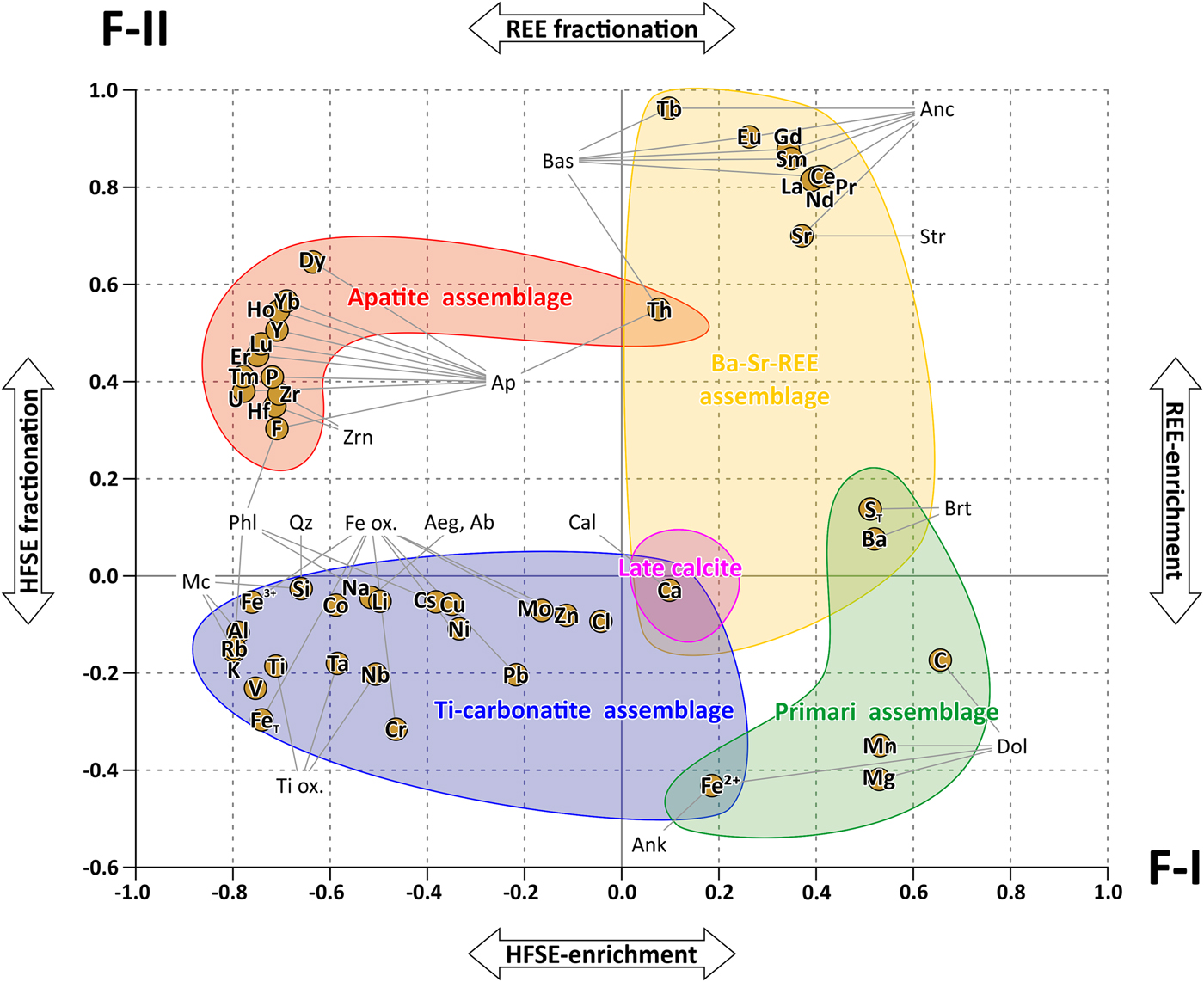
Figure 7. (Colour online) Positions of the points of studied major and trace elements on the factor plane formed by two “heaviest” factors. Abbreviations of the minerals are deciphered in the footnote of Table I. The fields limit the groups of elements associated with the minerals that belong to one or another identified mineral associations.
III. CONCLUSION
The use of factor analysis for a sufficiently large set of rock diffractograms (at least 40) makes it possible to determine the mineral composition of the entire collection at the level of rock-forming and minor minerals, even if they are present only in several samples of this set. The high resolution of the proposed approach is confirmed by the clear separation of Fe-dolomite and ankerite, which have extremely close positions of all of their lines. Additionally, we can learn about the peaks of each common diffractogram belonging to a particular mineral, as well as their exact position. The combination of these data facilitates quantitative XRPD by traditional methods and allows it to be performed quickly and correctly even for large sets of samples. The combination of analyses of mineralogical and geochemical data (1) simplifies the determination of minerals, (2) makes it possible to determine the effect of an identified mineral on the distribution of each element, and (3) allows us to link the results of the statistical processing of geochemical data with minerals and their associations. The “gathering” of minerals into one factor by the “and–and” type (the appearance of parasitic peaks and “crystallochemically forbidden” factor loadings) suggests their paragenetic connection. However, the method is quite sensitive to both the size of the sample set and the quality of diffraction data. The poor quality of primary data noticeably affects the interpretability of the results.
ACKNOWLEDGEMENTS
Analytical studies were conducted in the Geological Institute of Kola Science Centre RAS (GI KSC RAS), Tanaev Institute of Chemistry of Kola Science Centre (ICTREMRM KSC RAS), Institute of Geology of Karelian Research Centre RAS (IG KarRC RAS). All samples were collected and first processed by the authors with the help of V.V. Kirkin (AB MSTU), D.D. Mytsa, S.V. Petrov (IES SPbSU) and O.V. Kasanov (VIMS). Special thanks are to E.A. Selivanova (GI KSC RAS) for her useful tips. The authors express their sincere appreciation for the colleagues' kind assistance. T.A. Miroshnichenko (GI KSC RAS) significantly helped with English. Reviewer(s)” comments were very helpful. This work was supported by the Russian Foundation for Basic Research (project No. 18-35-00068) and carried out in the Geological Institute KSC RAS under the state order No. 0226-2019-0053.
Supplementary material
The supplementary material for this article can be found at https://doi.org/10.1017/S0885715619000435


