II. CRYSTALLITE SIZES – NUTS AND BOLTS

Assuming a theoretical spherical single crystallite of a defined size (e.g., diameter), the theoretical line profile can easily be calculated. The experimentally observed peaks however will be a convolution of the theoretical line profile and instrumental contributions. Therefore either a line profile standard, typically LaB₆, is measured to correct for the instrumental contribution or a convolution/fundamental parameter approach (Cheary and Coelho, Reference Cheary and Coelho1992) is used to deconvolute the physical line profile from the experimental line profile. Direct deconvolution methods such as the prominent method of Stokes (Reference Stokes1948) are less common nowadays since only non-overlapping peaks can be deconvoluted reasonably and an implementation of such methods in Rietveld compatible approaches is not easily possible.

After this fundamental step one can either try to simulate and match the physical line profile, for instance with the WPPM method or measure the line profile breadth using different methods. While there is considerable effort to implement the full power of the WPPM approach in Rietveld compatible approaches there are however without doubt still situations where physical line profile simulation is not the method of choice, e.g. in complex multiphase refinements with highly overlapping peak contributions. At the moment also the choice of anisotropic geometries in the WPPM approach is rather limited and restricted to some high-symmetric crystal systems owing to the complex nature of the CVFs (common volume functions) required for the simulation of accurate physical line profiles. To note that discrete geometries can however be considered numerically by the proposed algorithm of Leonardi et al. (Reference Leonardi, Leoni, Siboni and Scardi2012).

The later “measurement” methods have a long history of application in line profile analysis. The most commonly derived are the measure of the integral breadth (von Laue, Reference von Laue1936) and the variance (slope) (Tournarie, Reference Tournarie1956a, Reference Tournarieb; Wilson, Reference Wilson1962a) equivalent to the Fourier (Bertaut, Reference Bertaut1949a, Reference Bertautb) derived “size”. The attained values, the so-called apparent crystallite sizes of such measurements, have direct physical meanings and in most cases differ from each other. The apparent crystallite size ε _β derived from the measure of the integral breadth represents a volume-averaged mean thickness through the crystallite measured parallel to the scattering vector hkl. On the other hand, the apparent crystallite size ε _K from the measure of the variance slope (or from the Fourier method) represents a surface or area averaged mean thickness through the crystallite measured parallel to the scattering vector hkl (e.g., Langford and Wilson, Reference Langford and Wilson1978). These two measures are thus directly connected to a size parameter of the crystallite. Both measures can be related to the diameter of the crystallite D = 4/3*ε _β or D = 3/2*ε _K . The situation changes when considering a size distribution of spherical crystallites. Then still the relations hold 〈D _V〉 = 4/3*ε _β and 〈D _A〉 = 3/2*ε _K (e.g., Langford et al., Reference Langford, Louër and Scardi2000) but 〈D _V〉 is the so-called volume-weighted diameter and 〈D _A〉 is the so-called area (or surface)-weighted diameter. Those two diameters represent different moment quotients of the diameter distribution (thus produce different diameters or size parameters) and can be used to derive the later distributions if a certain distribution function type is assumed (e.g., the frequently observed or imposed lognormal distribution, Langford et al., Reference Langford, Louër and Scardi2000).

So far, only spherical crystallites are discussed here. The complexity rises by considering a large fraction of the crystallites to follow a certain morphology (e.g., an ellipsoid, a cylinder, or a cuboid). Numerous examples can be found concerning so-called nanorods, nanocubes, etc. in the nanoparticle area. Very often the orientation of such morphology is in equilibrium with the symmetry of the crystal system.

If the crystallites exhibit a certain morphology other than a sphere and a non-random orientation in the reciprocal lattice, then the apparent crystallite sizes ε _β and ε _K will be dependent on the hkl (or more specific be a function of hkl) of the respective Bragg peak since as stated earlier the average thicknesses are measured parallel to the scattering vector and will be different for each “direction” of view. This will effectively produce different breadths (and different physical line profiles) in dependence of hkl, known as anisotropic (size) peak broadening. Indeed powder diffraction using the Bragg peaks as information is the only non-imaging technique to provide such directional size information in contrast to small angle scattering and PDF (pair distribution function) techniques. A more detailed yet comprehensive discussion on the apparent crystallite sizes and influences on the physical line profile is available, e.g. in Wilson [Reference Wilson1962b; chapter IV].

The basic mechanism of the here discussed previously developed model (Ectors et al., Reference Ectors, Goetz-Neunhoeffer and Neubauer2015a, Reference Ectors, Goetz-Neunhoeffer and Neubauerb) is to calculate on the fly both ε _K and ε _β in dependence of the main radii r _x , r_y , and r _z of geometric shapes (Figure 1) in reference to spherical coordinates. The corresponding spherical coordinate system is then oriented in the reciprocal crystal system by defining two orthogonal reciprocal vectors hkl. In this way, all common crystal systems can be treated with the exact same approach. Once the orthogonal coordinate system of the geometric shape is properly oriented, the corresponding apparent crystallite sizes for each hkl are calculated constrained to the chosen geometrical shape and orientation.

Figure 1. (Color online) Geometric models (1) triaxial ellipsoid (2) elliptic cylinder (3) cuboid currently implemented in the AnisoCS and AnisoCSg macro with indicated directions of the main radii r _x , r_y , and r _z (figure created with OpenSCAD available at http://www.openscad.org).

The respective apparent crystallite sizes can then be used to directly calculate corresponding parameters of the size-Voigt-approximation (Ectors et al., Reference Ectors, Goetz-Neunhoeffer and Neubauer2015b). In this context, it is important to stress the important benefit of the double-Voigt approach allowing separate treatment of size and strain by two individual Voigt functions and the possibility to evaluate both the respective volume- and area-weighted apparent crystallite sizes simultaneously. Commonly available integral breadth methods require a combination with Fourier methods to measure both volume- and area-weighted apparent sizes and therefore depend critically on the accuracy of the two individual methods.

The previously developed model was implemented in the TOPAS (Bruker AXS Inc., Madison, WI, USA) Rietveld environment as an automated macro and is available free of charge in the supplemental material of Ectors et al. (Reference Ectors, Goetz-Neunhoeffer and Neubauer2015b) (see TOPAS macros file).

The next paragraph is intended to give practical advice how to properly parameterize and orient the geometric models in different crystal systems.

III. APPLICATION OF THE MODEL IN THE TOPAS ENVIRONMENT

The former macro is most conveniently stored in the local.inc file of the TOPAS environment. The framework consists of two refinement macros (AnisoCS and AnisoCSg) and two optional output macros. AnisoCS is the fundamental macro to call instead of the built-in macros for the isotropic size treatment (CS_L, CS_G, or LVol_FWHM_CS_G_L). AnisoCS calculates the area- or surface-weighted apparent crystallite sizes for each hkl of a structure (str) or the so-called hkl-phase in dependence of the chosen geometric model and refineable main radii in respect to the chosen orientation in the reciprocal lattice of a phase. For each hkl thus the Lorentzian integral breadth is strictly coupled to the refinement parameters. The additional AnisoCSg macro adds the Gaussian component to the Voigt size function in dependence of a refineable distribution parameter τ (see Ectors et al., Reference Ectors, Goetz-Neunhoeffer and Neubauer2015b for more details).

Since the Lorentzian part of the Voigt function always dominates the size broadening (Balzar and Ledbetter, Reference Balzar and Ledbetter1993), this order is meaningful. Indeed for practical application the consideration of the Lorentzian part only is frequently sufficient to dramatically improve the fit in case of anisotropic (size) broadening.

The correct input parameters for the macro are of huge importance for physical sound results. Therefore, the meaning of the respective refinement parameters will be discussed in detail.

The AnisoCS macro is for example called by:

AnisoCS(1, 0, 0, 1, 1, 0, 0, rx, 5, ry, 10, rz, 15, !pc, 0, !tc, 0, !nc, 0, 0).

The first number “AnisoCS(1”, is the choice of geometric model; 1 for an triaxial ellipsoid; 2 for an elliptic cylinder; 3 for a cuboid (rectangular parallelepiped). One should first consider a symmetry following model.

The following vector “AnisoCS(1, 0, 0, 1,” is the hkl vector of the Z -axis of the geometric model here ( 001 ). The Z -axis is also the special direction for the flat face of the cylinder model. The following vector “AnisoCS(1, 0, 0, 1, 1, 0, 0,” is hkl vector of the X -axis of the geometric model here ( 100 ). One has to make sure that both vectors are orthogonal to each other since the considered geometric models are orthogonal.

“AnisoCS(1, 0, 0, 1, 1, 0, 0, rx, 5, ry, 10, rz, 15,” are the variable names and initial values of the corresponding refineable main radii of the models. The parameter names can be freely chosen or coupled like for example “rx, 5, rx, 5, rz, 15”, in order to restrict the model here to a biaxial ellipsoid. Constraints can be applied in the normal TOPAS notation, e.g. “rx, 5 min=1; max=10.” One should again consider the symmetry of the crystal system.

“AnisoCS(1, 0, 0, 1, 1, 0, 0, rx, 5, ry, 10, rz, 15, !pc, 0, !tc, 0, !nc, 0, 0)” are the variable names and values of additional rotation of the model and the last “0”) is an orientation help in triclinic systems. These parameters and values should in conventional refinements not be modified or refined without the full awareness of the symmetry and possible cross-correlations (see Ectors et al., Reference Ectors, Goetz-Neunhoeffer and Neubauer2015a for details).

In summary, for routine application one should decide or test [In order to truly be able to differentiate between ellipsoids, cylinders, and cuboids a good statistic of independent observation directions (hkl) is needed.] the available models with meaningful radii parameterization and orientation of the geometric object according to the symmetry. However, symmetry breaking cases can also be treated but require a transformation of the crystal structure to the triclinic space group P1 (see Ectors et al., Reference Ectors, Goetz-Neunhoeffer and Neubauer2015a for details) since the multiplicities of respective hkl will be broken.

A symmetry following choice can easily be derived from basic crystallographic knowledge. An elegant way is however to use the so-called normal_plot option of TOPAS Version 5+ to visualize the refined or modeled morphology directly in order to judge if physical sound parameterization and orientation is present. For this purpose, the three considered geometric models have to be expressed mathematically in spherical coordinates. What seems an easy task is not as obvious as one might think for cylinders and cuboids. Derived from the so-called “superformula” (Gielis, Reference Gielis2003) in two dimensions and “superellipsoids” (e.g., Barr, Reference Barr1981) in three dimensions two adequate approximations were derived for the model radius in dependence of θ and φ as:

For an elliptic cylinder with the radii r _x , r_y , and r _z :

and for a cuboid, respectively:

These formulas can be “tuned” to even better representations (of the edges) of the geometric models by multiplying the magnitude of the exponents, but because of possible numerical overflows the described equations are sufficient approximations for displaying purposes.

For displaying the ellipsoid, the fact that ε _K of a triaxial ellipsoid-shaped crystallite is just another smaller ellipsoid is exploited in the following macro. For completeness a similar equation for a triaxial ellipsoid is:

The additional new macro for directly displaying the refined geometric model PlotAnisoCS for TOPAS reads:

Alongside with the Gaussian component (AnisoCSg) which is important for the derivation of respective size distributions a typical call of the macros for example for the refinement of a biaxial cylinder in a trigonal/hexagonal system would look like:

It is now indeed very simple to identify symmetry breaking parameterization of the geometric model and/or orientation as shown in Figure 2. Only proper parameterization and orientation will display the expected geometric model and thus will lead to sound results.

Figure 2. (Color online) (a) A properly oriented and parameterized cylinder in a trigonal crystal system. (b) The same cylinder with a wrong (non-orthogonal) X vector choice. (c) Attempt to fit an elliptic cylinder model in a trigonal crystal system. (d) Attempt to fit a cuboid model in a trigonal crystal system.

Clearly the normals_plot feature of TOPAS V5+ is not only a visual benefit, but also a very educative tool since additionally the plotting feature is aware of orientation thus displays the orthogonal geometric model in reference to the real-space lattice vectors (be aware that the orientation vectors Z and X are always chosen in reference to the reciprocal lattice vectors). Note also that the normal_plot option produces only normalized morphologies.

IV. SAMPLE CASE

In order to demonstrate the benefit of a routine treatment of pronounced anisotropic size peak broadening a commercially acquired hydrated lime sample was measured on a laboratory scale diffractometer and analyzed assuming an isotropic size model and a cylinder model for the portlandite phase. Effectively only one additional refinement parameter was introduced in reference to the isotropic refinement resulting in a severe drop of the R _wp factor and a clear improvement of the fit quality as can be observed in Figure 3.

Figure 3. (Color online) (a) Refinement of the hydrated lime sample with an isotropic crystallite size model. Severe misfits are visible for the (010/012/110) peaks of portlandite at approximately (28.7/47.1/50.8°2θ). Notably a Pawley-refinement does not solve the misfits. (b) Refinement of the hydrated lime sample with the cylinder crystallite size model. A biaxial ellipsoid model was also tested but resulted in a slightly higher R _wp value of 4.94%. R _exp is 3.09% for both refinements.

Portlandite being a typical layered structure normal to c* is often observed to crystallize in pseudo-hexagonal platy prisms which is in good agreement with the displayed morphology. The refined microstructure parameters indicate a negligible strain (“maximum strain” e0 of 0.072%) and respective area (or surface)-weighted cylinder diameter in the (hk0) direction of 46.9 nm and height in (00l) of 9.6 nm with volume-weighted counterparts corresponding to 76.0 and 15.6 nm, respectively. The high ratio (1.62) between the volume- and area-weighted values indicate a rather broad size distribution. These values and the resulting morphology should without further evidence always be interpreted as effective values and morphology, since it cannot be claimed that the proportions of the aspect ratio is necessarily a constant in real samples. Technically one would have to consider a distribution of diameters and heights separately still with the assumption that the orientation and shape is invariant.

This sample demonstrates how the addition of only one additional physical sound size parameter efficiently can improve the fit dramatically as indicated by the reduction of the R _wp from 7.16 to 4.78% and the R _Bragg of the used (room temperature) portlandite structure [space group P $\bar 3$ m1, refined lattice parameters a 3.5895(1) and c 4.9108(1) Å, from Henderson and Gutowsky, Reference Henderson and Gutowsky1962] from 2.26 to 0.86%.

For completeness the two used initial macro calls:

V. ACCURACY

In this paragraph, the accuracy of the developed model to physical line profiles is evaluated by fitting simulated data by means of the WPPM approach as realized in the PM2K (Leoni et al., Reference Leoni, Confente and Scardi2006) software. In order to evaluate the accuracy of the Voigt approximation to the line profile using a isotropic case under common laboratory conditions three different lognormal distributions widths, from narrow to broad, with three individual size ranges were simulated in a cubic crystal system with a step size of 0.01°2θ CuKα using the PM2K software. Evaluation was done using TOPAS Version 5 with an appropriated so-called hkl phase. The profile calculation and weighting options of TOPAS were kept to the default setting. The refined parameters in this case were the respective radii r _x for a spherical model, the distribution parameter τ and individual scale factors for the individual peaks. A total of nine simulated distributions were evaluated with area-weighted sphere diameters of 10, 50, and 100 nm and corresponding volume-weighted counterparts of 1.1 (called narrow), 1.3 (called medium), and 1.5 (called broad) times the area-weighted diameters, respectively. The reason to choose those two variation parameters is on the one hand that approaching the 100 nm region the Bragg peaks get very narrow frequently cited as being the limiting “size” for reasonable evaluation. On the other hand, with the lognormal distributions getting very broad the respective Gaussian contribution dramatically decreases, leading to so-called super-Lorentzian peak shapes (Balzar and Ledbetter, Reference Balzar and Ledbetter1993). Such behavior is not observed with the other frequently assumed γ distributions (Popa and Balzar, Reference Popa and Balzar2002).

In general, we expect the size evaluation to be reasonable if the deviation from the simulated value is within approximately 10% relative. Figure 4 displays the results of the derived area- and volume-weighted sphere diameters. The error bars indicate the 10% error range from the simulated values.

Figure 4. (Color online) Results of the fitting of the AnisoCS and AnisoCSg macros to simulated sphere distributions from the WPPM method. Error bars indicate the 10% relative error range from the simulated values.

It can be clearly observed from Figure 4 that all refined sizes are very reasonably in the range of the simulated values. Only the results from broad distributions are slightly outside the 10% criterion. The highest deviation (13.5%) in the area-weighted diameters is a refined 8.7 nm in respect to the simulated 10.0 nm. The highest deviation (9.4%) in the volume-weighted diameter being a refined 135.8 nm in respect to the simulated value of 150.0 nm. In awareness of the approximation of the physical line profile by a Voigt function, the results can be considered very reasonable.

Of course, more interesting in the scope of this paper is the accuracy when considering anisotropic crystallite sizes, since the former results also can be obtained using the implemented procedures in TOPAS or with the double-Voigt approximation, still it is of course of importance to be aware of the range of approximation of the double-Voigt approach.

In order to evaluate the accuracy of anisotropic cases, including size distributions two sets of cylinders in a trigonal/hexagonal crystal system were again simulated using the WPPM approach as realized in PM2K. In this case, lognormal distributions were chosen to reflect a ratio of 1.2 for the volume-weighted to area-weighted cylinder diameters and heights. The cylinder height (00l) to diameter (hk0) ratio was varied from 0.25 up to 4. The two size ranges were evaluated, namely with area-weighted cylinder diameters of 10 nm (referred to as the 10 nm series) and 50 nm (referred to as the 50 nm series). The fitting results are visualized in Figure 5.

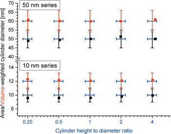
Figure 5. (Color online) Results of the fitting of the AnisoCS and AnisoCSg macros to simulated cylinder distributions with different height-to-diameter ratios from the WPPM method. Error bars indicate the 10% relative error range from the simulated values. Black squares and red dots represent the attained area- and volume-weighted cylinder diameters, respectively. The height-to-diameter ratio on the x-scale is constant for both area- and volume-weighted cylinder diameters (x-scale in log₂ scaling for display purposes).

Clearly the results of Figure 5 demonstrate that the refinement method for anisotropic crystallites is in good agreement with the simulated line profiles. The largest discrepancy in the height on diameter is observed at the cylinder distributions with area-weighted diameters of 50 nm with a corresponding cylinder height of 200 nm (cylinder height on diameter 4). This demonstrates that the practical limit for reasonable size evaluation is as often cited in the range of 100–200 nm.

VI. ACCURACY IN PRESENCE OF ISOTROPIC STRAIN

So far, microstrain-free simulations have been evaluated. The practical difficulty is however often the deconvolution of size and strain effects. The double-Voigt approach is perfectly suitable for such deconvolution without further analysis procedures required. In order to evaluate again in a practical way the efficiency of the later approach the already considered distributions of cylinders were resimulated with the inclusion of isotropic microstrain. For that purpose one can understand isotropic microstrain as a distribution of lattice parameters. The simulated isotropic strain contribution was therefore achieved by inclusion of a discrete symmetric triangular-like function to the relative d-values as visualized in Figure 6. The corresponding maximum deviation from the reference lattice parameters is ±0.7% relative.

Figure 6. The used d-value dispersion distribution in order to simulate an isotropic strain contribution.

In Figure 7, the corresponding refined results with a refined strain contribution (Gaussian & Lorentzian strain contributions freely refined) are visualized.

Figure 7. (Color online) Results of the fitting of the AnisoCS and AnisoCSg macros to simulated cylinder distributions with different height-to-diameter ratios and isotropic microstrain from the WPPM method. Error bars indicate the 10% relative error range from the simulated values. Black squares and red dots represent the attained area- and volume-weighted cylinder diameters, respectively. The height-to-diameter ratio on the x-scale is constant for both area- and volume-weighted cylinder diameters (x-scale in log₂ scaling for display purposes).

While the results of 10 nm series display good agreement the 50 nm series displays still acceptable results, only with the very high cylinder height (200 nm) showing a deviation outside the defined criterion. This can be very well understood since in the 10 nm series the size effect on the peak broadening is dominating; however, in the 50 nm series the microstrain broadening is a very dominant effect as shown in Figure 8.

Figure 8. (Color online) Comparison of selected simulated diffraction pattern of the 10 and 50 nm series displaying the effect of the isotropic strain contribution. Note that the 10 nm series with and without strain contribution is almost superimposed.

When neglecting the cylinder distribution with area-weighted diameters of 50 nm with a corresponding cylinder height of 200 nm the results fit very well in the defined 10% margin. The average derived “maximum strain” e0 of the 10 nm series is 0.19(1)% and for the 50 nm series 0.20(2)%, which is in reasonable agreement of the expected value from the simulation of 0.1875% in the e0_(FWHM) definition used by the TOPAS software.

When erroneously no strain is considered very visible misfits were observed. Inclusion of the strain refinement, e.g. of the 10 nm series lead to a drop of the R _wp in the range of 43–88% relative.

The deconvolution of isotropic microstrain in the double-Voigt approach critically depends on the presence of at least one well-resolved second-order reflection. Fits without second-order reflection in the 10 nm series produced maximum deviations of 43.2, 31.4, and 40.2% for the area-weighted diameters, volume-weighted diameters, and cylinder height on width, respectively. Inclusion of only one second-order reflection reduced the maximum deviations down to very reasonable 9.8, 4.0, and 5.6%, respectively. This demonstrates the absolute need of an appropriate angular 2θ measurement range for meaningful microstructure analysis in general.

VII. LIMITATIONS OR A WORD OF WARNING

In microstructure analysis from powder diffraction methods, the degree of information available is always limited and depends on the degree of approximation one is willing to accept. The assumption that the line profile produced from the size effect is a Voigt function of course does not hold. It is a reasonable approximation in most practical cases but will never be able to produce accurate results in all theoretical cases. As far as the double-Voigt approximation is concerned size and morphology effects can be treated with the proposed model on a physical sound basis and even in the case of isotropic strain deconvolution is reasonably successful. Yet, a physical account for “anisotropic” strain contribution as introduced e.g. by dislocations or non-uniform lattice parameter deviations is at the moment not realized to the author's knowledge in a usable way in the double-Voigt approach though it may, as far as the line profile approximation methods allow, be the model of choice.

Even within the 10% relative error scale derived size distributions can vary very noticeably if a certain distribution function is postulated since the “measureable” area- and volume-weighted parameters are ratios of the higher moments of the distribution. Therefore slight differences in derived distributions should always receive very careful consideration and in the best case should be validated against other microstructure analysis methods or transmission electron microscopy.

The intention of the demonstrated model for anisotropic size treatment is to account in a physically sound, parameter efficient, fast and stable way the considered effects in routine Rietveld refinements.