In June 2014, the civil war in Iraq reached a turning point when the “Islamic State of Iraq and the Levant” (ISIL) group captured seven major cities in the northern part of the country.Footnote 1 The Kurdish-dominated areas in Iraq and Syria have been traditionally calmer in both war-torn countries and neither international organizations nor governments had seen this escalation coming. This episode demonstrates that regions at risk in ongoing conflicts are hard to identify even under the watchful eye of the international community. With the recent uprisings of the Arab Spring, the ongoing violence in Iraq and Afghanistan, and numerous conflicts in central Africa, ISIL’s advances will not be the last geographic expansion of conflict with disastrous humanitarian consequences.
The question therefore springs to mind whether and to what extent the scholarly research program on irregular conflicts can help us to predict major conflict zones in civil wars in advance. Recent empirical research on the spatial determinants of violence in civil conflict has generated substantial insights. Theoretically, the failure of states to control their remote periphery has been repeatedly used as an explanation for political violence (Herbst Reference Herbst2000; Fearon and Laitin Reference Fearon and Laitin2003; Herbst Reference Herbst2004; Buhaug, Gates and Lujala Reference Buhaug and Gates2009; Scott Reference Scott2009). Drawing on these insights, a series of studies has combined Geographic Information Systems and multivariate regression designs to test related hypotheses (Buhaug and Gates Reference Buhaug and Rød2002; Buhaug and Rød Reference Buhaug, Gleditsch, Holtermann, Østby and Tollefsen2006; Buhaug, Gates and Lujala Reference Buhaug and Gates2009). Moreover, properties of irregular conflicts have also been modeled in disaggregated computational studies drawing on geographic information (see Bhavnani, Miodownik and Nart Reference Bhavnani, Miodownik and Nart2008; Bhavnani et al. Reference Bhavnani, Donnay, Miodownik, Mor and Helbing2013; Weidmann and Salehyan Reference Weidmann, Kuse and Gleditsch2013).
Despite this progress in combining theoretical and quantitative insights, the external validity and in particular the predictive capabilities of this research program remain understudied. On the country level, quantitative predictions of political instability have made substantial progress in recent years (see Goldstone et al. Reference Goldstone, Bates, Epstein, Gurr, Lustik, Marshall, Ulfelder and Woodward2010; Ward et al. Reference Ward, Metternich, Dorff, Gallop, Hollenbach, Schultz and Weschle2013). Beyond their practical utility of informing relief organizations and policy decision, predictions offer scientific benefits as they directly communicate the degree to which a studied phenomenon is understood (Ward, Greenhill and Bakke Reference Ward, Greenhill and Bakke2010; Schrodt Reference Schrodt2014).
Another advantage of predictions is that they are not restricted to the empirical sample: predicting locations of violent conflict beyond the sample that the model was fitted on reveals to what extent the data-generating mechanism and relevant variables were correctly identified. Based on these considerations, this paper tests to what extent geographic covariates of irregular warfare that have been identified in previous work improve predictions of conflict zones. To evaluate these predictions, I rely both on a quantitative and a qualitative metric. Spatial predictions of conflict intensities are compared with empirically observed intensities to calculate error scores. Moreover, high-intensity conflict regions yielding >50 percent of the maximal conflict intensity are compared visually with empirically observed hot spots.
The merit of this exercise is twofold: first, a direct comparison between the predictions of models and random baselines serves as a reality check for the geographic research program, clearly communicating to what extent informed predictions outperform random guesses. Second, the applied methodology generates easily communicable predictions that could be utilized beyond basic research to aid planning of humanitarian relief operations, for example.Footnote 2
To demonstrate the predictive capabilities of the associated variables, point process models (PPM) are used to predict instances of lethal violence in ten recent insurgencies in Sub-Saharan Africa. Predictions of these models are compared with the empirical record using an innovative cross-validation design. The results indicate that central variables of the geo-quantitative research program lead to drastically improved out-of-sample predictions in comparison with uniform baselines.
Literature Review
The connection between geography and war has long been considered important. Already the classic literature of revolutionary warfare and counterinsurgency devoted attention to the topic (see Guevara Reference Guevara1961, 10; Mao [1938] Reference Mao1967; McColl Reference McColl1969). Contemporary research has stressed the primarily local determinants of fighting in civil conflicts (Buhaug and Gates Reference Buhaug and Rød2002; Buhaug and Rød Reference Buhaug, Gleditsch, Holtermann, Østby and Tollefsen2006; O’Loughlin and Witmer Reference O’Loughlin and Witmer2010; Buhaug et al. Reference Buhaug, Gates and Lujala2011; Rustad et al. Reference Rustad, Buhaug, Falch and Gates2011). While regular armies generally move and fight under central command, irregular conflicts are frequently fought out between local militias and rebel supporters. Instead of strategic decisions of where to send mechanized armies to fight, local encounters between irregular fighters and military units determine much of the violence in civil conflicts (Kalyvas Reference Kalyvas2005).Footnote 3
A series of publications has been devoted explicitly to coding and explaining the location, size, and extent of primary conflict zones in armed conflict. Buhaug (Reference Buhaug2010) applies a distance-decay model from the study of interstate war to internal conflicts and finds that the relative military strength of the belligerents is a strong predictor for the location of primary conflict zones. Drawing on a bargaining perspective, Butcher (Reference Butcher2014) analyzes the location of conflict zones and concludes that multilateral sub-national conflicts tend to occur more in the periphery. Braithwaite (Reference Braithwaite2010) analyzes under which conditions hot spots of international armed conflict are likely to emerge. Hallberg (Reference Hallberg2012) contributes a geo-referenced data set on primary conflict zones in civil wars since 1989. The recent turn toward more disaggregated empirical studies has led to an increased interest in data on single conflict events (Raleigh and Hegre Reference Raleigh and Hegre2005; Sundberg, Lindgren and Padskocimaite Reference Sundberg, Lindgren and Padskocimaite2011) and geo-referenced data on local determinants of conflict intensity. Consequently, geographic and local socioeconomic conditions have moved into the focus of empirical studies. Drawing on spatially disaggregated data on wealth and data on conflict events, Hegre, Østby and Raleigh (Reference Hegre, Østby and Raleigh2009) found that violence tends to cluster in more wealthy regions, possibly because rebels prioritize them in their attacks. Raleigh and Hegre (Reference Raleigh and Hegre2009) also found that population concentrations generally see higher levels of fighting. While the statistical association is strong, it remains unclear how this effect comes about. A relatively constant per capita rate of violence as well as strategic targeting of civilian concentrations spring to mind as possible explanations.
While the emphasis on local determinants of conflict is justified both theoretically and empirically, the diffusion of irregular civil conflict over time has also been studied. Schutte and Weidmann (Reference Schutte and Weidmann2011) investigated different diffusion scenarios for violence in civil wars, comparing instances of empirical diffusion against random baseline scenarios. Zhukov (Reference Zhukov2012) used road-network information in a refined empirical analysis and found that violence in the north Caucasus tended to relocate over time along roads. Both studies point to the fact that a substantive number of civil war events result from previous fighting in neighboring regions rather than being solely caused by local conditions. Beyond spatial expansion, reaction to specific instances of violence has also been analyzed (Lyall Reference Lyall2009; Kocher, Pepinsky and Kalyvas Reference Kocher, Pepinsky and Kalyvas2011; Braithwaite and Johnson Reference Braithwaite and Johnson2012; Schutte and Donnay 2014). Again, reactive patterns in conflict event data underline that the conflict history as well as local socioeconomic and geographic conditions jointly affect levels of violence in civil wars.
In summary, the presented literature on the determinants of violence in civil conflicts suggests an interaction of multiple factors. Strategically, the military capabilities of the actors as well as terrain conditions and infrastructure play an important role for the locations of major battle zones. On a tactical level, violence tends to cluster as actors fight repeatedly over specific locations, but it also diffuses into previously unaffected regions. Finally, the types of violence applied by actors in the field crucially affects subsequent levels of violence. While these insights are important for testing and building theories of the dynamics of violence in irregular conflict, the question of whether or not they translate into generalizable and ultimately actionable knowledge remains unanswered. Regression studies and matching designs are generally used to test whether or not specific variables have a causal effect in line with theoretical considerations. The estimated effects, however, relate solely to hypothetical all-else-being-equal, or “ceteris paribus” scenarios.
Despite the obvious merit of inferential designs, the added scientific and practical value of predictions has been pointed out in recent publications (Goldstone et al. Reference Goldstone, Bates, Epstein, Gurr, Lustik, Marshall, Ulfelder and Woodward2010; Ward, Greenhill and Bakke Reference Ward, Greenhill and Bakke2010; Gleditsch and Ward Reference Gleditsch and Ward2012; Schrodt Reference Schrodt2014). Tangible predictions about the location and timing of violence are a concern of policy makers and relief organizations. Consequently, political scientists have embarked on generating predictions for which countries are likely to experience civil wars (Goldstone et al. Reference Goldstone, Bates, Epstein, Gurr, Lustik, Marshall, Ulfelder and Woodward2010; Ward, Greenhill and Bakke Reference Ward, Greenhill and Bakke2010; Weidmann and Ward Reference Weidmann and Salehyan2010; Ward, Greenhill and Bakke Reference Ward, Metternich, Dorff, Gallop, Hollenbach, Schultz and Weschle2013) and which regions are most prone to violence in Afghanistan (Zammit-Mangion et al. Reference Zammit-Mangion, Dewar, Kadirkamanathan and Sanguinetti2012). Advancing this line of research, this paper is a first attempt to predict major conflict zones across civil conflicts. The performance of these predictions is assessed in comparison with random baselines. In essence, this paper communicates how much predictive power the quantitative research program on the micro-dynamics of civil wars has gained in comparison with agnostic guessing about where violence will occur. This exercise serves as an important reality check for our ability to predict sub-national conflict intensity based on central variables identified in the literature.
Of course, assessing the predictive performance of these variables requires a suitable empirical setup. The paper proceeds as follows: in the next section, I will discuss the case selection for this study. After that, I will identify central variables for the prediction of variation in conflict intensity from the above-referenced literature. A generic setup for predicting violence based on these variables is presented in the subsequent section, loosely based on Zammit-Mangion et al. (Reference Zammit-Mangion, Dewar, Kadirkamanathan and Sanguinetti2012). Finally, I will test whether and to what extent these variables produce improved out-of-sample predictions in comparison with agnostic baselines.
Scope and Case Selection
Because the literature on revolutionary warfare and counterinsurgency studies have been most vocal in proposing a direct link between rebel presence and terrain conditions, I decided to narrow down the empirical analysis to insurgencies, that is, conflicts in which the rebels are not recognized as belligerents and heavily rely on civilian assistance to wage a guerrilla war against the state (Galula Reference Galula1964; CIA 2009, 2). However, not all civil or irregular conflicts are insurgencies. Kalyvas and Balcells (Reference Kalyvas and Balcells2010) report a declining trend for this type of conflict and an increase in wars that blend elements of conventional fighting with irregular rebellions. Moreover, fighting in quasi-conventional civil wars, such as in Yugoslavia in the early 1990s, might be better predicted by ethnic boundaries than terrain conditions. Despite the overall decline in the frequency of insurgencies, they still constitute the most frequent type of armed conflict in the post-World War II period. Conflict events from the “Geo-Referenced Event Dataset” (GED) (Sundberg, Lindgren and Padskocimaite Reference Sundberg, Lindgren and Padskocimaite2011) cover lethal clashes that occurred between 1990 and 2010 from 42 African countries. Drawing on a separate data set by Lyall and Wilson (Reference Lyall and Wilson2009), I identified 11 cases of insurgency that are covered in GED.Footnote 4 I decided to exclude Djibouti (1991–2001) because the country is too small for meaningful geographic analysis, given the resolution of the covariates. Table 1 shows the remaining cases that were used for the analysis.
Table 1 Overview of the Cases Used for the Statistical Analysis

Note: Start- and end-dates correspond to the first and last observations in the GED data set for the corresponding conflicts.
Due to the exclusive coverage of African conflicts in GED, the generated insights might capture aspects that are specific to the region: for example, Herbst (Reference Herbst2000, 21–31) argues that low average population densities, porous colonial borders, and capital city locations close to the shore shaped fundamental aspects of the African state system. In comparison with Europe, less competition over territory between nation-states can be seen, while controlling the remote periphery of the states’ territories posed a bigger challenge. Therefore, the geographic determinants of fighting in insurgencies could be more important in Africa than in other regions. Future research based on global event data might show whether the results generalize beyond Africa.
Spatial Determinants of Fighting
The localized nature of fighting in civil conflicts provides a suitable starting point for predictive modeling. Recent studies have utilized digital information on geographic conditions and conflict events to reveal a series of robust statistical relationships. I will therefore introduce conflict event data sets and data on the spatial determinants of violence that have been identified by previous studies to systematically test to what extent predictions of conflict intensity can be improved by each variable.
Geographic Data on Armed Conflict
In the past decade, several data collection efforts have been started to disaggregate civil conflicts into a series of events. These events range from skirmishes to major battles or atrocities against civilians. Both the “Armed Conflict Location and Event Dataset” (ACLED) (see Raleigh and Hegre Reference Raleigh and Hegre2005) as well as the GED (see Sundberg, Lindgren and Padskocimaite Reference Sundberg, Lindgren and Padskocimaite2011) rely on news reports that contain information on violent events primarily in Sub-Saharan Africa. GED is based on an elaborate coding procedure that ensures reliability by cross-validating records with multiple coders (Sundberg, Lindgren and Padskocimaite Reference Sundberg, Lindgren and Padskocimaite2011). Definitions of what constitutes a conflict event vary slightly between the data sets: in ACLED, violence against civilians as well as battle outcomes such as changes in territorial control are recorded. Sporadically, ACLED also has information on initiators of violence, but information on casualties is not recorded. GED is restricted to lethal encounters between political actors and provides estimates for civilian and military casualties. Information on both outcomes of battles and initiators are missing. For this study, I used the GED data set on lethal events in African civil conflicts between 1990 and 2010. The advantage of GED for this particular project is that lethal encounters are particularly relevant and conceptually clear. In the next sections, I will introduce covariates to predict spatial variation in lethal violence in insurgencies.
Population
Based on the notion of “population-centric warfare” (see CIA 2009, 2), civilian population concentrations have been identified as a predictor of conflict events (Raleigh and Hegre Reference Raleigh and Hegre2009). Insurgents seek contact with the civilian population for various reasons: to hide from incumbent forces (Salehyan and Gleditsch Reference Salehyan2006), to recruit additional combatants (Sheehan Reference Sheehan1988, 50), and to extend their geographic control over relevant parts of the country (Kalyvas Reference Kalyvas2006, 202–7). Spatially disaggregated population counts from the Gridded Population of the World dataset (CIESIN 2005) were therefore included in the predictive models.
Distances to capital and border
The ultimate goal of irregular uprisings is to conquer the capital city, as was the case in Saigon in 1975, in Kabul in 1996, and in Monrovia in 2003. Defending the center is therefore a strategic imperative for the state. Repeated attempts to attack the government and incumbent counteractions make distance to the capital city a spatial predictor of higher levels of violence (see Buhaug, Gates and Lujala Reference Buhaug and Gates2009; Buhaug Reference Buhaug2010; Toellefsen, Strand and Buhaug Reference Toellefsen, Strand and Buhaug2012). Along the same lines, distance to the nearest international border that provides refuge to the rebels has been associated with levels of violence (Salehyan Reference Salehyan and Gleditsch2009; Buhaug Reference Buhaug2010). Cases in point are the Vietcong that moved their vital supply lines partially to Laos and Cambodia and the Afghan Mujaheddin that traditionally fight superpowers from bases in the border regions in Pakistan. Distances to capital cities and international boundaries were calculated based on Weidmann, Kuse and Gleditsch (Reference Weidmann and Ward2010).
Accessibility
Remote and difficult terrain provides insurgents with the opportunity to prepare attacks and temporarily evade the fighting (Fearon and Laitin Reference Fearon and Laitin2003). In order to counterbalance the material superiority of the state, rebels utilize less accessible areas to prepare military operations and recruit from the local population (McColl Reference McColl1969). Terrain and soil conditions, road and railroad networks, bodies of water, and forested regions all affect the accessibility of sub-national regions. A comprehensive aggregation of these factors has been performed by Nelson (Reference Nelson2008). Their provision of a global friction map for traveling times between all cities with >50,000 inhabitants in the year 2000 offers a suitable operationalization for infrastructural accessibility.
Wealth
Spatial variation in wealth has been associated with conflict events (Hegre, Østby and Raleigh Reference Hegre, Østby and Raleigh2009). Two principal scenarios are imaginable for this variable to affect levels of violence. First, materially deprived regions could see stronger support for insurgent activities. Second, rebels might strategically target wealthier regions for private gains and/or to finance the uprising. Lootable resources in particular have been linked to intense standoffs in civil conflicts (Gilmore et al. Reference Gilmore, Gleditsch, Lujala and Rød2005). Spatially disaggregated data on wealth (Nordhaus Reference Nordhaus2006) codes disaggregated GDP data on a global scale. The derived unit is gross cell product: an estimate for the market value of all goods and services in a geographic region. Cells with a maximal size of 60 nautical square miles (about 111 km2) are coded in this data set, which was also included. While the exact causal roles of these geographic factors remain disputed, general correlations between the corresponding variables and levels of violence are widely accepted.
Natural land cover
Densely forested regions can be as inaccessible as high mountain ranges. Consequently, they severely limit situation awareness and mobility for regular forces (see Crawford Reference Crawford1958). In Columbia, the FARC rebels have evaded defeat for almost four decades, Ugandan LRA rebels are still at large despite regional and international attempts to stop their activities, and Vietnamese rebels waged three successful campaigns against three different global powers between 1941 and 1975. In all of these cases, dense forestation has been cited as an important enabler of guerrilla actions. I therefore included a data set that codes the percentage of green vegetation for the year 2001 on a global scale and with a spatial resolution of 1 km2 (Broxton et al. Reference Broxton, Zeng, Scheftic and Troch2014).
While the exact causal roles of these geographic factors remain disputed, general correlations between the corresponding variables and levels of violence are widely accepted. But to what extent are these factors capable of predicting the spatial variation of the intensity of violence in civil wars? As mentioned above, this paper seeks to provide an easily communicable answer to this question. The next section details the corresponding approaches to modeling and validation.
Modeling Approach
Several possible modeling approaches spring to mind for predicting conflict events based on the presented data. Many contemporary studies of violence in civil wars draw on econometric analyses. While the breadth of econometric methodology and the rapid rate at which it advances cannot be overlooked, the analysis of inherently spatial data introduces problems. First and most importantly, the nature of the dependent variable—conflict events distributed in space—has no obvious equivalent in the econometrician’s toolbox. Researchers therefore usually aggregate event counts within spatial units such as artificial grid cells and then apply count-dependent variable models (see, e.g., Fjelde and Hultman Reference Fjelde and Hultman2013; Pierskalla and Hollenbach Reference Pierskalla and Hollenbach2013; Basedau and Pierskalla Reference Basedau and Pierskalla2014). Unfortunately, in most cases there is no empirically or theoretically informed strategy for choosing the sizes of such cells.
Of course, statistical predictions both in- and out-of-sample also hinge (to some extent) on design decisions in the spatial aggregations as defined by the chosen grid cells and their origin. Moreover, within the possibly large cells, event are analyzed independently from their exact location. These insights leads Cressie (Reference Cressie1993, 591) to the conclusion that “[t]he reduction of complex point patterns to counts of the number of events in random quadrats and to one-dimensional indices results in a considerable loss of information.”
This presents a serious problem for the ambition of this paper: if the claim was made that out-of-sample predictions of conflict intensity were possible based on a grid-cell approach, this finding would partly be due to an ad hoc choice of a specific cell size. Moreover, precise local information would be given up in favor of aggregate covariate values at the cell level.
Ideally, a non-parametric technique would be used for mapping conflict events to covariate information. To address this issue, an alternative modeling approach more frequently chosen in biology and epidemiology relies on PPM. While PPM have been applied to conflict research before (Zammit-Mangion et al. Reference Zammit-Mangion, Dewar, Kadirkamanathan and Sanguinetti2012), the relative novelty of this approach requires a more in-depth discussion of their properties. The next section gives an overview of PPM and their application to multivariate inference, as well as the chosen setup for prediction, cross-validation, and extrapolation.
PPM
Before discussing this type of model in further detail, some terminology needs to be introduced. Spatial point patterns are generally analyzed within clearly demarcated areas. These areas are referred to as “windows” and can be either artificial geometric structures or irregularly shaped polygons. In this study, the country polygons obtained from Weidmann, Kuse and Gleditsch (Reference Weidmann and Ward2010) are used as observational windows with one model being fitted per country.
Statistical models of spatial point patterns have been developed for several decades and successfully applied to various fields, such as biology, geography, and criminology. One obvious quantity of interest in spatial point patterns is their intensity, defined as the expected number of points per area in a given spatial window. The intensity of the point process can vary continuously within the window as a function of covariates or another point pattern. While the introduction of a temporal dimension provides additional challenges, PPM are attractive alternatives to econometric models for cross-sectional analyses of conflict events. Their main advantage is that they offer empirically driven and non-parametric solutions for selecting the area around the points for aggregating covariate information. In the next section, I will introduce some implementational details of PPM starting with underlying assumptions. After that, I will provide a closer look at fitting these models to data.
Underlying assumptions for spatial Poisson processes
Any quantitative model must strike a balance between mathematical tractability and theoretical adequacy. Very much in favor of the first requirement for this application is the spatial Poisson process, which can serve as a suitable starting point for predictive modeling. For the spatial variant of the Poisson process, two principal sub-types must be distinguished: homogeneous and inhomogeneous processes. In the case of the homogeneous spatial Poisson process, the intensity (i.e., the number of points per area) λ is uniform for the entire observational window. Of course, modeling high- or low-intensity areas within countries requires the intensity to vary as a function of covariates.
The introduction of subregions within the spatial window is a way to achieve this. A heuristic method for choosing subregions for a given empirical point pattern will be discussed in the next section. For each of the subregions, covariate values can be established and used to estimate marginal effects. Points per subregion are Poisson-distributed with probability mass function for natural positive numbers X and k:
 $${\rm Pr}(X\,{\equals}\,k)\,{\equals}\,{{\lambda ^{k} } \over {k\,!\,}}e^{{{\minus}\lambda }} .$$
Across regions, however, the intensity of the Poisson processes may vary and the numbers of points per subregion are independent (see Baddeley and Turner 2005, 72ff.). Applying this formalism to the study of civil conflict does justice to the strand of literature that points to the local determinants of violence. However, it omits the well-described escalatory dynamics of violence and spatial diffusion.Footnote 5 For the spatial modeling, this also entails that the approach is prone to overdispersion: the variance encountered in empirical event intensity is larger than the variance predicted by the Poisson models. This is due to the fact that mean and variance are characterized by the same variable (λ) in the Poisson distribution. However, this study focuses on predicting the average intensity of violence in a given region and not the variance in intensity.
Poisson process models therefore serve as an eligible point of departure for predictive purposes and do not require ad hoc design decisions about the spatial scale of point-to-point interactions.
Choosing tiles for covariate information
Modeling point intensity as a function of geographic covariates requires that the points in the empirical sample are associated with the covariate information. As mentioned before, PPM does not rely on predefined spatial units to achieve this and instead choose suitable tiles heuristically from the point pattern. As illustrated in Figure 1, this is accomplished in two steps: first, a number of “dummy” points are superimposed on the empirical point pattern. They are either arranged in a grid-like structure (as shown in Figure 1 on the right), or are uniformly distributed at random. In a second step, the study window is divided into tiles which are either associated with dummy points or empirical ones. The tiling algorithm is usually chosen to optimally demarcate regions that are closest to the empirical or simulated points, for example, by calculating Dirichilet tiles (i.e., Voronoi diagrams; see Mitchell Reference Mitchell1997, 233). For each of the resulting tiles, covariate information is then aggregated. Of course, the exact tiles resulting from the tessellation are still dependent to some extent on the number of dummy points in the sample and their spatial distribution. However, the great advantage of this approach is that covariate values that are subsequently used for model fitting are obtained from areas that are closer to the empirical points than the simulated dummies. This is arguably a better approach to mapping covariate information to empirical points than an arbitrary spatial grid with empirically uninformed cell size and origin.

Fig. 1 Illustration of a quadrature scheme based on Dirichilet tessellation Source: Figure taken from Baddeley and Turner (Reference Baddeley and Turner2000).
Fitting models to data
For the estimation of β-parameters, the applied tessellation techniques usually generate tiles intersecting with points in the sample and a comparable number of tiles for areas without points. A widely used approach for fitting point patterns to data relies on the Berman–Turner algorithm (see Algorithm 1), which implements a maximum pseudo-likelihood approach to parameter estimation: instead of choosing parameters based on their likelihood, Berman and Turner (Reference Berman and Rolf1992) suggest choosing them according to their conditional intensity—that is, the observed number of points per area in the tiles given the estimated intensity. Berman and Turner (Reference Berman and Rolf1992) observe that the conditional intensity of the inhomogeneous spatial Poisson process has the same functional form as likelihood functions employed in generalized linear models (GLM). This allows for a wide range of PPM to be fitted in readily available GLM software. In detail, Berman and Turner (Reference Berman and Rolf1992) suggest the following setup:

Being able to fit models to data is a central prerequisite for assessing the predictive gain associated with individual variables. In the next section, I will introduce the remaining requirements: a general error score to compare prediction and empirical data and a cross-validation setup for out-of-sample tests.
Error Score
To keep the validation approach as general as possible, I decided to simulate point patterns from the fitted prediction models and then compare them with the empirical patterns.Footnote 6 Of course, simulated point patterns vary from simulation run to simulation run as they are generated probabilistically. To establish average predictions, I simulated point patterns from the fitted models 100 times for each in-sample and out-of-sample test. A suitable method that yields a continuous non-parametric estimate for the point process was described by Diggle (Reference Diggle1985).Footnote 7 I decided to compare simulated and empirical intensities numerically to assess the performance of different models.
While this setup might look rather cumbersome at first glance, it essentially generates a side-by-side comparison between empirically estimated and simulated intensities. This direct comparison communicates the performance of the models in a straightforward manner and easily generalizes to other models such as more advanced PPM, agent-based models, or grid-cell-based econometric models. Figure 2 depicts empirical and simulated conflict events, as well as corresponding intensity surfaces.

Fig. 2 Example of empirical and simulated events from the Second Liberian Civil War (1999–2003)Note: On the top left, the empirical events from the Geo-Referenced Event Dataset can be seen for this conflict. On the top right, a corresponding Gaussian intensity estimation is visible. In the bottom row, simulated events and the corresponding surface are depicted.
The prediction error is computed based on the absolute differences in the densities for empirical and simulated events. Density surfaces are represented as fine-grained arrays. The mean absolute error for an array with J cells is calculated as follows:
 $${\rm MAE}\,{\equals}\,{{\mathop{\sum}\limits_1^J {\rm abs}(emp_{j} {\minus}sim_{j} )} \over J}.$$
Figure 3 illustrates the comparison and the calculation of average prediction errors visually.

Fig. 3 Depiction of the error metric used for the prediction models Note: The two lines are the cross sections of the point intensity estimates for empirical and simulated point patterns. The differences in densities (gray areas) are approximated numerically.
In this setup, the total number of events is still given by the empirical sample, that is, the specific county the model was fitted on. Of course, predicting the overall number of conflict events (i.e., the severity of the civil war) is not in the focus of this study. Numerous socioeconomic, political, and military factors influence the severity of conflicts and it would be impossible to do justice to them in this article. I therefore decided to normalize the predicted intensities to one. As a result, the predictions reflect relative intensities scaled from 0 to 1.
Cross-Validation
In order to assess the predictive capabilities of the fitted models out-of-sample, a suitable cross-validation setup had to be defined as well. Basically, cross-validation works by dividing the available empirical sample into a training and a test set. Models are fitted on the training set and then used to generate predictions for the test set. Those predictions are then validated against the empirically observed results from the test set. This setup serves as a more realistic test framework than simply assessing the in-sample predictions of statistical models—that is, their ability to replicate the test data they were trained on.Footnote 8
In this case, I chose to apply a leave-one-out cross-validation scheme.Footnote 9 Models were fitted on all but one of the countries in the statistical sample. A prediction model was generated by averaging the β-coefficients of these models. The resulting model was subsequently used to predict the point pattern in the remaining country. This setup mimics the real-world challenge of predicting the spatial distribution of violence in future civil wars based on a set of historical conflicts. In the next section, I will present results for predictions of conflict intensity for all ten African cases.
Results
In order to assess the predictive capabilities of the models, I computed density differences both in-sample and out-of-sample. For the in-sample assessment, I fitted a series of Poisson models based on the introduced covariates and fitting techniques using the spatstat package for the R programming language. I simulated 100 distinct point patterns from the fitted models and calculated intensity surfaces. One expected density for each model was established by averaging over these simulations. Table 2 shows cumulative differences between the empirical density and the average simulated density. To generate a baseline against which the models could be compared, I generated 100 random point pattern consisting of an equal number of points as the empirical sample. The average difference in normalized intensities between random and empirical patterns serve as a baseline against which the predictions can be compared.
Table 2 In-Sample Results Based on Differences Between Normalized Empirical and Simulated Intensities

In-Sample Prediction
In total, seven model predictions plus the random baseline were simulated for each country. As a first test of the introduced setup and the predictive capabilities of the models, the introduced variables were added subsequently to the model specification. Acronyms in the top row of the prediction tables indicate the variables that were used: “p” stands for population, “c” for capital distance, “a” for accessibility, “w” for wealth, “b” for border distance, and “v” for vegetation. Results from a full-fledged model-averaging setup where each covariate’s predictive performance is tested against a series of different model specifications are presented in the supplementary information.Footnote 10 Table 2 shows cross-validation scores for the different model specifications and the random baseline. As discussed above, these scores are the average cumulative absolute difference between the empirical and the simulated point patterns. The last row in the table shows normalized cross-validation scores across countries with the random baseline having a value of 1. This row shows that the initial models that only use population as a predictor already yield half the cumulative error scores (0.45) of the random baseline. As additional predictors are introduced, the scores drop from 0.27 to 0.22. This setup also shows that not every predictor yields the same improvements. Model 2, using data on population centers and capital distances, clearly outperforms model 1, but subsequent additions of predictors only yield marginal returns.Footnote 11 Model 3 with an error score of 0.22 performs best in this setup. These results are encouraging as they demonstrate that the introduced data and modeling techniques can be used to replicate empirical patterns to some extent. However, the real test for the presented setup are predictions beyond the sample that the models were fitted on. Corresponding results can be found in Table 3.
Table 3 Cross-Validation Results for Predictions that were Fitted on Nine of the Ten Countries and then Used to Predict the Remaining Country

Out-of-Sample Prediction
Table 3 shows scores based on the leave-one-out cross-validation setup described in Cross-Validation section. As one would expect, the cumulative error score across models is higher than in the in-sample setup (3.90 compared with 3.84). However, the out-of-sample predictions generally perform surprisingly well: for all but the simple population model, error scores below 0.3 of the normalized random baseline errors are attained. Interestingly, the lowest error scores are achieved for models 3, 4, and 7 which only include three to four predictors each. The slightly lower performance of models 5 and 6 might be due to overfitting. Generally, the out-of-sample predictions work well and serve as a powerful reminder of the achievements of geographic and quantitative research on civil conflicts of the last decade. While measuring deviations between empirical and predicted densities is a good way to quantify the performance of prediction models, qualitative comparisons as introduced in the next section add another important angle to the empirical analysis.
Qualitative Comparisons
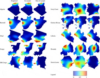
The final section of this paper shows side by side comparisons of Empirical Densities and Predictions. For each of the ten countries in the sample, three plots were generated. The plots on the left show normalized intensity surfaces for the empirical patterns. The columns in the middle and on the right show model predictions based on model 7, which had the lowest error scores in the in-sample and out-of-sample predictions. In the middle column, model 7 was fitted on the country under investigation. In the right column, the cross-validation model based on the estimates of the remaining cases was used to predict the country under investigation. The associated legend can be found below the country plots. As seen in Side-By-Side Comparisons of Empirical Densities and Predictions section, most of the out-of-sample predictions actually predict high-conflict areas. This is remarkable, as it both underscores the merit of the used data sets as well as the validity of the chosen modeling approach. These specific predictions also illustrate the merit of the technology for informing relief organizations and policy.
But how can we explain the fact that some conflicts are predicted quite well while others are not? A closer look at the (qualitatively) most obvious mispredictions—Ivory Coast and Republic of the Congo—can provide some answers. In the Ivorian case, the framework of a peripheral insurgency slowly advancing toward the center simply does not apply very well. Instead, ethnic and religious tensions between an predominantly Christian South and a predominantly Muslim North account for a large fraction of the conflict events (see McGovern Reference McGovern2011). This entailed that the region of high-intensity fighting occurred along an East-West axis, while the model predictions place it in the northern periphery (see predictions in Side-By-Side Comparisons of Empirical Densities and Predictions section).
In the case of the Republic of Congo, much of the fighting happened during the height of the civil war in and around the capital city, Brazzaville. Fearing the outcome of a July 1997 Presidential election, followers of the top candidates Pascal Lissouba and Col. Denis Sassou Nguesso engaged in an armed struggle over control of the capital (see DeRouen and Heo Reference DeRouen and Heo2007, 129). While the uprising against then-ruling President Lissouba qualifies as a popular insurgency given the participation of numerous irregular fighters, Mao’s ([1938] Reference Mao1967) three-stage model for peripheral insurgencies fails to apply. Instead of building on a protracted and peripheral campaign, the warring parties opted for a conflict option that could be better described as a popular coup d’état. Instead of affecting remote areas, the fallout in political violence of this conflict clustered around the capital city in the far south of the country.
In contrast, the correctly predicted conflict zone in Burundi emerged from an insurgency that fits the proposed theoretical framework quite well. As Vorrath (Reference Vorrath2010, 101) observes “one specific feature of the Burundian civil war was that the Hutu rebels never seized a larger territory inside the country, but followed a guerrilla strategy of moving in and out. This was facilitated by the fact that the Hutu rebel groups had bases abroad, namely in Tanzania and the Congo.” Arguably, the presence of an international border close to Burundi’s capital city Bujumbura and the concentration of population in the area were contributing factors to the clustering of conflict events in the region. In this case, the assumptions underlying the modeling framework line up with the conflict scenario.
Discussion and Conclusion
Studies of armed conflict have identified a number of geographic conditions that correlate with guerrilla activity. Both protection from state power in terms of remoteness and the presence of strategic targets such as population centers affect the probability of armed clashes taking place in insurgencies. Causal effects of selected spatial covariates have been analyzed by a flurry of recent publications. However, established effects were only valid for specific spatial units, and only hold under ceteris paribus conditions. An assessment of the external validity of this research program has been missing so far. Filling this gap, this paper has used geographic data on conflict as well as a series of theoretically prominent geographic covariates to predict the spatial distribution of conflict, both in-sample and out-of-sample. The results clearly communicate to what extent these variables actually improve predictions in direct comparison with an agnostic baseline: in-sample, cumulative error scores only amount to 25 percent of the cumulative error of the random baseline. In out-of-sample predictions, the error scores are slightly higher, but they still only amount to <30 percent of the random baseline error. In qualitative comparisons, the locations of high-intensity conflict zones are correctly predicted in six out of ten countries. Two countries (Sierra Leone and the Democratic Republic of the Congo) have two distinct high-intensity conflict areas, and only one of them is predicted correctly. In the two remaining countries (Ivory Coast and Republic of Congo) the predictions are incorrect. While more work needs to be done to identify and test predictors of violence and include more advanced modeling techniques, these results underscore the external validity of the insights generated by geo-quantitative research on civil conflicts and their potential merit for real-world applications.
Side-By-Side Comparisons of Empirical Densities and Predictions