


Since the mid-1980s, different variants of configurational comparative methods (CCMs) have gradually been added to the toolkit for causal data analysis in the social sciences. CCMs are designed to investigate different hypotheses and uncover different properties of causal structures than traditional regression analytical methods (RAMs) and, thus, complement the latter (rather than compete with them). RAMs examine covariation hypotheses as “the more/less of X, the more/less of Y” that link variables, and they quantify net-effects and effect sizes. CCMs, by contrast, study implication hypotheses as “X=χ i is (non-redundantly) sufficient/necessary for Y=γ i” that link specific values of variables. Moreover, instead of quantifying effect sizes, CCMs place a Boolean ordering on sets of causes by locating their elements on the same or different causal paths to the ultimate outcome. In other words, while RAMs investigate the quantitative properties of causal structures as characterized by statistical or probabilistic theories of causation (e.g., Suppes Reference Suppes1970), CCMs scrutinize their Boolean properties as described by regularity theories of causation (Mackie Reference Mackie1974).
The Boolean properties of causation encompass three complexity dimensions. The first is conjunctivity: to bring about an effect, say, liberal democracy in early modern Europe (D=1), different factors need to be instantiated (or not instantiated) jointly; for instance, according to Downing’s (Reference Downing1992) theory of the origins of liberal democracy, a country must have a history of medieval constitutionalism (C=1) and absent military revolutions (R=0). Only a coincident instantiation of the conjunction C=1∗R=0 produces the effect D=1. Disjunctivity is a second complexity dimension: an effect can be brought about along alternative causal paths. Downing (Reference Downing1992, 78–9, 240) identifies four paths leading to the absence of military revolution (R=0): a geography that deters invading armies (G=1), commercial wealth (W=1), foreign resource mobilization (M=1), and foreign alliances (A=1). Each condition in the disjunction G=1 + W=1 + M=1 + A=1 can bring about the effect R=0 independently of the other conditions. The third complexity dimension is sequentiality: effects tend to cause further effects, propagating causal influence along causal chains. In Downing’s theory there are multiple chains, for instance, W=1 is causally relevant to R=0, which, in turn, is causally relevant to D=1, or there is a chain from A=1 via R=0 to D=1. Overall, the theory entails the following Boolean causal model (cf. Goertz Reference Goertz2006, 254), where “→” stands for the Boolean operation of implication:
 $$(G\equals}1{\;\plus\;}W{\equals}1{\;\plus\;}M{\equals}1{\;\plus\;}A{\equals}1{\,→\,} R{\,\!\equals}0)\;{\vskip -2pt ∗}\;(C{\equals}1{\vskip -2pt ∗}R{\equals}0{\,→\,} D\!\!{\,\,\equals}\!1).$$
The most prominent CCM is Qualitative Comparative Analysis (QCA; Ragin Reference Ragin2008). While the original variant of QCA introduced in Ragin (Reference Ragin1987), crisp-set QCA (csQCA), is restricted to modeling dichotomous variables, there meanwhile exist fully worked out variants that can process multi-value variables, multi-value QCA (mvQCA) (Cronqvist and Berg-Schlosser Reference Cronqvist and Berg-Schlosser2009), and variables with continuous values from the unit interval, fuzzy-set QCA (fsQCA) (Ragin Reference Ragin2009). However, all QCA variants focus on the complexity dimensions of conjunctivity and disjunctivity only, as QCA treats exactly one factor as endogenous and all other analyzed factors as exogenous. QCA will thus not find a chain model as (1).Footnote 1
In light of this restriction, Baumgartner (Reference Baumgartner2009) introduced a new CCM called Coincidence Analysis (CNA). As a member of the family of CCMs, CNA—just like QCA—investigates implication hypotheses and scrutinizes the Boolean properties of causation. Contrary to QCA, however, CNA is capable of analyzing multi-outcome structures and, hence, of uncovering all Boolean complexity dimensions. CNA is tailor-made to recover chain models as (1).
So far, though, CNA has only been available in a crisp-set variant (csCNA). This paper removes that limitation by generalizing the method for multi-value variables (mvCNA) and variables with continuous values from the unit interval that are interpreted as membership scores in fuzzy-sets (fsCNA). This generalization comes with a major adaptation of the basic algorithmic protocol on the basis of which CNA builds causal models. In a nutshell, while CNA so far—just like QCA—adopted a top-down approach to model building that first identifies complete sufficient and necessary conditions of outcomes and then gradually eliminates redundant elements, the generalized variant of CNA uses a bottom-up approach that progressively combines factor values to complex but redundancy-free sufficient and necessary conditions.
The CNA algorithm presented here has been implemented in a new version of the R package cna, version 2.1.1 (Ambühl and Baumgartner Reference Ambühl and Baumgartner2018), which makes the whole inferential power of mvCNA and fsCNA available to end-users. By drawing on this software package and the currently most reliable R package for QCA, QCApro (Thiem Reference Thiem2018),Footnote 2 the paper also performs a whole battery of benchmark tests that evaluate and compare the performance of CNA and QCA when applied to data with varying forms of data deficiencies. The test series reveals that the reversal of the basic model building approach gives CNA an edge over QCA not only with respect to multi-outcome structures but also with respect to the analysis of non-ideal data stemming from single-outcome structures.
The paper is organized as follows. We first introduce the theoretical background of CNA along with its main input parameters. Next, the generalization of the CNA algorithm is presented. The final section then reports the results of the test series evaluating and comparing CNA and QCA. The online appendix contains supplemental information on configurational homogeneity and correctness and provides charts with all numeric results of our test series. A replication script detailing all analytical steps is available in the PSRM dataverse.
Theoretical background
Boolean difference-making
As all CCMs, CNA searches for causal dependencies as defined by so-called regularity theories of causation, whose development dates back to David Hume (Reference Hume1999 [1748]). Modern regularity theories define causation in terms of Boolean difference-making within a fixed causal background. More specifically, X=χ i is a regularity theoretic cause of Y=γ i if there exists a (fixed) configuration of background conditions  $\scr{F}$ such that, in $\scr{F}$, a change from X=χ k to X=χ i, where χ i≠χ k, is systematically and non-redundantly associated with a change from Y=γ k to Y=γ i, where γ i≠γ k. If X=χ i does not make a difference to Y=γ i in any context $\scr{F}$, X=χ i is redundant to account for Y=γ i and, thus, no cause of Y=γ i (Mackie Reference Mackie1974; Graßhoff and May Reference Graßhoff and May2001; Baumgartner Reference Baumgartner2013).
To render that idea more precise, some conceptual preliminaries are required. Regularity theoretic causation holds between variables/factors taking on specific values. (We will use the terms “variable” and “factor” interchangeably.) Factors represent categorical properties that partition sets of units of observation (cases) either into two sets, in case of binary properties, or into more than two (but finitely many) sets, in case of multi-value properties. Factors representing binary properties can be crisp-set (cs) or fuzzy-set (fs); the former can take on 0 and 1 as possible values, whereas the latter can take on any (continuous) values from the unit interval. Factors representing multi-value properties are called multi-value (mv) factors; they can take on any of an open (but finite) number of possible values {0,1,2, … ,n}. Values of a cs or fs factor X are interpretable as membership scores in the set of cases exhibiting the property represented by X. As is conventional in Boolean algebra, we shall abbreviate membership in a set by upper case and non-membership by lower case Roman letters; that is, we write “X” for X=1 and “x” for X=0. An alternative interpretation, which lends itself particularly well for causal modeling, is that “X” stands for the presence of the factor X and “x” for its absence. In case of mv factors, we will not abbreviate value assignments and, instead, use the explicit “Variable=value” notation by writing, say, “X=3” for X taking the value 3.
Apart from the Boolean operations of conjunction, disjunction, and negation, whose classical definitions are presupposed here, the implication operator “→” and the equivalence operator “↔” are of core importance for the regularity theoretic definition of causation. According to a classical interpretation, an expression as “X=3→Y=4” states that whenever X takes the value 3, Y takes 4; or “X→Y” states that whenever X is present, Y is present. These claims are true if, and only if (iff), there is no case satisfying the left-hand side of “→” and not satisfying the right-hand side. Furthermore, “X=3 ↔ Y=4” and “X↔Y” are true iff the implication holds both ways, meaning that all cases satisfying the left-hand side of “↔” also satisfy the right-hand side, and vice versa.
For the subsequent generalization of CNA for fs factors the classical Boolean operations must be translated into fuzzy logic. There exist numerous systems of fuzzy logic (for an overview cf. Hájek Reference Hájek1998), each of which comes with its own rendering of Boolean operations. We will adopt the following fuzzy-logic renderings, which have become standard in the context of CCMs: conjunction X∗Y is defined in terms of the minimum membership score in X and Y, that is, min(X,Y), disjunction X + Y in terms of the maximum membership score in X and Y, that is, max(X,Y), negation ¬X (or x) in terms of 1−X, an implication X→Y is taken to express that the membership score in X is smaller or equal to Y (X≤Y), and an equivalence X↔Y that the membership scores in X and Y are equal (X=Y).
Based on the implication operator the notions of sufficiency and necessity are defined, which are the two Boolean dependencies exploited by regularity theories: X is sufficient for Y iff X→Y holds; and X is necessary for Y iff Y→X holds. Analogously, the more complex expression X=3 + Z=2 is sufficient and necessary for Y=4 iff X=3 + Z=2 ↔ Y=4 holds.
Boolean dependencies of sufficiency and necessity amount to mere patterns of co-occurrence of factor values; as such, they carry no causal connotations whatsoever. In fact, most Boolean dependencies do not reflect causal dependencies. For that reason, regularity theories rely on a non-redundancy principle as an additional constraint to filter out those relations of sufficiency and necessity that are due to underlying causal dependencies: A Boolean dependency structure is causally interpretable only if it does not contain any redundant elements. Causes are those elements of sufficient and necessary conditions for which at least one configuration of background conditions $\scr{F}$exists in which they are indispensable to account for a scrutinized outcome. In other words, whatever can be removed from sufficient and necessary conditions without affecting the latter’s sufficiency and necessity is redundant and, therefore, not causally interpretable. Only sufficient and necessary conditions that are completely free of redundant elements, viz. minimal, possibly reflect causation (Baumgartner Reference Baumgartner2015).
Boolean causal models
Modern regularity theories formally cash this idea out on the basis of the notion of a minimal theory. Its complete definition is intricate and beyond the scope of this paper (for the latest definition see Baumgartner and Falk Reference Baumgartner and Falk2018). For our subsequent purposes, the following rough characterization will suffice. There are atomic and complex minimal theories. An atomic minimal theory of an outcome Y is a minimally necessary disjunction of minimally sufficient conditions of Y. A conjunction Φ of coincidently instantiated factor values (e.g., X 1∗X 2∗ … ∗X n) is a minimally sufficient condition of Y iff Φ is sufficient for Y (Φ→Y), and there does not exist a proper part Φ' of Φ such that Φ'→Y. A proper part Φ' of Φ is the result of eliminating one or more conjuncts from Φ. A disjunction Ψ of minimally sufficient conditions (e.g., Φ1 + Φ2 + … + Φn) is a minimally necessary condition of Y iff Ψ is necessary for Y (Y→Ψ), and there does not exist a proper part Ψ' of Ψ such that Y→Ψ'. A proper part Ψ' of Ψ is the result of eliminating one or more disjuncts from Ψ. Overall, an atomic minimal theory of Y states an equivalence of the form Ψ↔Y (where Ψ is an expression in disjunctive normal formFootnote 3 and Y is a single factor value). Atomic minimal theories can be conjunctively concatenated to complex minimal theories.
Minimal theories connect Boolean dependencies, which—by themselves—are purely functional and non-causal, to causal dependencies: those, and only those, Boolean dependencies that appear in minimal theories can stem from underlying causal dependencies. Atomic minimal theories stand for causal structures with one outcome, complex theories represent multi-outcome structures. To further clarify the causal interpretation of minimal theories, consider the following complex exemplar:
 $$(A{\vskip -2pt ∗}b\,{\plus}\,a{\vskip -2pt ∗}B \,↔ \,C)\;{\,\vskip -2pt ∗\,}\;(C{\vskip -2pt ∗}f\,{\plus}\,D\,↔ \, E).$$
Functionally put, (2) claims that the presence of A in conjunction with the absence of B (i.e., b) as well as a in conjunction with B are two alternative minimally sufficient conditions of C, and that C∗f and D are two alternative minimally sufficient conditions of E. Moreover, both A∗b + a∗B and C∗f + D are claimed to be minimally necessary for C and E, respectively. Against the background of a regularity theory, these functional relations entail the following causal claims: (i) the factor values listed on the left-hand sides of “↔” are directly causally relevant for the factor values on the right-hand sides; (ii) A and b are located on the same causal path to C, which differs from the path on which a and B are located, and C and f are located on the same path to E, which differs from D’s path; (iii) A∗b and a∗B are two alternative indirect causes of E whose influence is mediated on a causal chain via C. More generally put, minimal theories ascribe causal relevance to their constitutive factor values, place them on the same or different paths to the outcomes, and distinguish between direct and indirect causal relevancies. That is, they render transparent the three Boolean complexity dimensions of causality—which is why we shall likewise refer to minimal theories as Boolean causal models.
Two fundamentals of the interpretation of Boolean causal models must be emphasized. First, ordinary Boolean models make claims about causal relevance but not about causal irrelevance. With some additional constraints that are immaterial for our current purposes (for details see Baumgartner Reference Baumgartner2013), a regularity theory defines X 1 to be a cause of an outcome Y iff there exists a fixed configuration of context factors $\scr{F}$=X 2∗ . . . ∗X n in which X 1 makes a difference to Y—meaning that X 1∗$\scr{F}$ and x 1∗$\scr{F}$ are systematically associated with different Y-values. While establishing causal relevance merely requires demonstrating the existence of at least one such difference-making context, establishing causal irrelevance would require demonstrating the non-existence of such a context, which is impossible on the basis of the non-exhaustive data samples that are typically analyzed in observational studies. Correspondingly, the fact that, say, G does not appear in (2) does not imply G to be causally irrelevant to either C or E. The non-inclusion of G simply means that the data from which model (2) has been derived do not contain evidence for the relevance of G.
Second, Boolean models are to be interpreted relative to the data set δ from which they have been derived. They do not purport to reveal all of an underlying causal structure’s Boolean properties but only detail those causally relevant factor values along with those conjunctive, disjunctive, and sequential groupings for which δ contains evidence. By extension, two different Boolean models mi and mj derived from two different data sets δ i and δ j are in no disagreement if the causal claims entailed by mi and mj stand in a subset relation. For example, model (3) does not conflict with model (2):
 $$(A{\plus}B\,↔ \, C)\;{\vskip -2pt ∗}\;(C{\plus}D\,↔ \, E).$$
(3) identifies A and B as alternative direct causes of C and indirect causes of E, moreover C and D are claimed to be alternative direct causes of E. All of this also follows from (2). The causal claims entailed by (3) thus constitute a subset of the claims entailed by (2). The two models describe properties of one and the same underlying causal structure at different degrees of detail and relative to different data δ (2) and δ (3).
Data, consistency, coverage
CCMs analyze configurational data δ that have the form of m×k matrices, where m is the number of units of observation (cases) and k is the number of factors. We subsequently refer to the set of factors F in an analyzed δ as the factor frame of the analysis. While QCA requires that F be partitioned—prior to the analysis—into a first subset {Y} comprising exactly one endogenous factor and a second subset F\{Y} comprising all exogenous factors of the analysis, CNA can dispense with such a partition. If prior causal knowledge is available as to what factors in F are possible effects and what factors can be excluded as effects, this information can be given to CNA via an optional argument called a causal ordering. A causal ordering is a relation Xi≺Xj defined on the elements of F entailing that X j cannot be a cause of X i (e.g., because X i is instantiated temporally before X j). If an ordering is provided, CNA only searches for Boolean models in accordance with the ordering; if no ordering is provided, CNA treats all values of the factors in F as potential outcomes and explores whether a causal model for them can be inferred from δ.
As real-life data tend to feature noise induced by unmeasured causes of endogenous factors, strictly sufficient or necessary conditions for an outcome Y often do not exist. To still extract some causal information from such data, Ragin (Reference Ragin2006) has imported consistency and coverage measures (with values from the interval [0,1]) into the QCA protocol. Both of these measures are also serviceable for the purposes of CNA. Informally put, consistency (con) reproduces the degree to which the behavior of an outcome obeys a corresponding sufficiency or necessity relationship or a whole model, whereas coverage (cov) reproduces the degree to which a sufficiency or necessity relationship or a whole model accounts for the behavior of the corresponding outcome (for formal definitions see the vignette of the cna package, Ambühl and Baumgartner Reference Ambühl and Baumgartner2018, §3.2.) If no (strictly Boolean) relations of sufficiency and necessity with con=1 and cov=1 can be inferred from δ, CNA invites its users to lower the consistency and coverage thresholds con t and cov t. For example, by lowering con t to 0.8, CNA is given permission to treat X as sufficient for Y, even though in 20 percent of the cases X is not associated with Y. Or by lowering cov t to 0.8, CNA is allowed to treat X as necessary for Y, even if 20 percent of the cases featuring Y do not feature X.
Lowering con t and cov t must be done with great caution, for the lower these thresholds, the higher the chance that causal fallacies are committed. In QCA, however, it is common to only impose lowest bounds—for example, 0.75—for the consistency of configurations comprising all exogenous factors, so-called minterms. This approach does not guarantee that the consistencies of issued minimally sufficient conditions (or prime implicants, as they are called in QCA) and of resulting Boolean models are also above the chosen threshold. Accordingly, the models output by QCA often do not meet the consistency threshold set by the user (cf. the replication script for examples). Moreover, it is common QCA practice not to require lowest bounds for coverage. In consequence, QCA models frequently cover less than half of the cases featuring the outcome in δ.
In CNA, the consistency and coverage standards are higher—for two reasons. First, the sufficient conditions that are ultimately causally interpreted by CCMs are not minterms (which are mere intermediate calculation devices for QCA) but redundancy-free conditions contained in Boolean models. Hence, consistency thresholds must be imposed on the latter, not on the former. Second, a model’s coverage being low means that it only accounts for few instances of an outcome in δ. Or differently, in many cases in δ where the outcome is present there are causes at work that are not contained (i.e., unmeasured) in the factor frame F. However, unmeasured causes tend to confound δ—in particular, when they are associated with both exogenous and endogenous factors in F. The presence of confounders casts doubts on the causal interpretability of all dependencies manifest in δ, for uncontrolled causes might be covertly responsible for them. That is, the more likely it is that the data are confounded, the less reliable a causal interpretation of resulting models becomes. The higher the coverage, the less likely it is that we are facing data confounding, the more reliable a causal interpretation of issued models becomes. The online appendix A provides an extended discussion of the conditions under which CNA can be expected to output correct models.
Generalizing the CNA algorithm
Top-down versus bottom-up search
The goal of CCMs is to infer Boolean causal models from configurational data. The previous section has shown that Boolean functions are amenable to a causal interpretation only if they identify redundancy-free sufficient and necessary conditions, and thus amount to minimal theories that reach imposed consistency (con t) and coverage (cov t) thresholds.
There exist two different strategies for building minimal theories: they can be built from the top down or from the bottom up. The top-down approach proceeds as follows. First, complete sufficient minterms are identified that meet con t; second, elements are eliminated as redundant as long as the remaining conditions continue to satisfy con t; third, the minimally sufficient conditions are disjunctively combined to necessary conditions that meet cov t; fourth, elements are eliminated as redundant that are not required to satisfy cov t. By contrast, the bottom-up approach starts with single factor values and tests whether they meet con t; if that is not the case, it proceeds to test conjunctions of two factor values, then to conjunctions of three, and so on. Whenever a conjunction meets con t (and no proper part of it has previously been identified to meet con t), it is automatically redundancy-free, that is, a minimally sufficient condition (msc), and supersets of it do not need to be tested for sufficiency any more. Then, the bottom-up approach tests whether single msc meet cov t; if not, it proceeds to disjunctions of two, then to disjunctions of three, and so on. Whenever a disjunction meets cov t (and no proper part of it has previously been identified to meet cov t), it is automatically redundancy-free, viz. a minimally necessary condition, and supersets of it do not need to be tested for necessity.
Both QCA and the original variant of csCNA adopt versions of the top-down approach—albeit in very different algorithmic implementations (cf. Baumgartner Reference Baumgartner2015). By contrast, the generalization of CNA developed here reverses the direction of model building. Prima facie, it might seem that it does not matter whether models are built from the top down or from the bottom up because both directions should ultimately lead to the same results. Although that is indeed the case for some data types, in particular for ideal data, it does not hold generally. For instance, when applied to data that do not allow for modeling outcomes with perfect consistency, it can happen that—contrary to the bottom-up approach—the top-down approach does not succeed in eliminating all redundancies from sufficient conditions. The reason is that when building models from the top down it is (implicitly) presumed that consistency threshold violations are monotonic in the following sense: if a factor C cannot be eliminated from a sufficient condition A∗B∗C because A∗B alone does not meet con t, then C plus some further factor from A∗B cannot be eliminated either. Therefore, if eliminating C from A∗B∗C leads to a violation of con t, the top-down approach concludes that C is needed to account for the outcome, meaning C is a difference-maker. That conclusion, however, is not valid, because consistency threshold violations are not monotonic.
To see this, consider the data matrix in Table 1A, for which the following consistencies hold:
 $$\eqalignno{ & con(A{\,\vskip -2pt\!∗}B{\,\vskip -2pt ∗}C \, → \, D){\equals}{\scale85%{\raise0.7ex\hbox{${3}$} \!\mathord{\left/ {\vphantom {3 4}}\right.\kern-\nulldelimiterspace}\!\lower0.7ex\hbox{$4$}}}{\equals}0.75 \cr & \hskip 12.5ptcon(A\!{\,\vskip -2pt ∗}B \, → \, D){\equals}{\scale85%{\raise0.7ex\hbox{$8$} \!\mathord{\left/ {\vphantom {8 {11}}}\right.\kern-\nulldelimiterspace}\!\lower0.7ex\hbox{${11}$}}}{\equals}0.73 \cr & \hskip 22pt con(A \, → \, D){\equals}{\scale85%{\raise0.7ex\hbox{${15}$} \!\mathord{\left/ {\vphantom {{15} {20}}}\right.\kern-\nulldelimiterspace}\!\lower0.7ex\hbox{${20}$}}}{\equals}0.75 $$
Table 1 Problem Cases for the Top-down Approach

That is, if con t is set to 0.75, the condition A∗B∗C, which is sufficient for D with con=0.75, satisfies the threshold. By contrast, A∗B, which results from A∗B∗C by eliminating C, falls short of con t. Nonetheless, further eliminating B lifts the remaining condition above con t again, as A alone is sufficient for D with con=0.75. That means, while C initially appears to be a non-redundant element of the sufficient condition A∗B∗C, it turns out to be redundant after all. The top-down approach, however, only tests the removability of single factors at a time and infers that a condition is redundancy-free if removing single factors would push that condition below con t. Therefore, at con t=0.75, a procedure that adopts the top-down approach as QCA issues model (4) for Table 1A.
 $$A\!{\,\vskip -2pt ∗}b\!{\,\vskip -2pt ∗}c\,{\plus}\,A\!{\,\vskip -2pt ∗}B\!{\,\vskip -2pt ∗\,}\!C \, → \, D\quad con{\equals}0.83;cov{\equals}0.67.$$
In contrast, by first testing whether single factors meet con t, the bottom-up approach directly finds that A itself is sufficient for D. Moreover, it turns out that A is necessary for D, as it accounts for D with perfect coverage. Overall, at con t=0.75, a procedure that builds models from the bottom up issues model (5).
 $$A\,↔ \, D\quad con{\equals}0.75;\;cov{\equals}1.$$
(5) is preferable to (4), for two reasons. First, the product of consistency and coverage, which is a common measure for overall model fit, is significantly higher for (5). Second, model (5) only ascribes causal relevance to A, whereas (4) also determines B, C and their negations to be causes of D, even though the data in Table 1A do not contain evidence that these factors actually make a difference to D at con t=0.75. Hence, when applied to noisy data, the top-down approach runs a risk of drawing causal inferences that go beyond the data.
Also, the top-down approach may abandon an analysis prematurely. To see this, consider the fs data in Table 1B, where D is the outcome.Footnote 4 The four configurations in that data have the consistencies listed in the last column of the QCA truth table in Table 1C, meaning that, if con t is set to 0.75, none of the configurations are sufficient for the outcome. A top-down procedure as QCA abandons the analysis at this point. That, however, is unwarranted because there in fact exists a Boolean model for D that meets con t=0.75 and moreover reaches perfect coverage:
 $$A\!{\,\vskip -2pt ∗\,}\!B\,↔ \, D\quad con{\equals}0.78;\;cov{\equals}1.$$
By starting the analysis with single factors, the bottom-up approach finds model (6) in the second iteration.
To avoid the problems of the top-down approach, the generalization of CNA developed in this paper builds models from the bottom up.
The essentials of the CNA algorithm
The generalized CNA algorithm takes as mandatory inputs (i) a data set δ, (ii) con t and cov t thresholds, and (iii) an upper bound called maxstep for the maximal complexity of atomic solution formulas (atomic causal models) to be built. Maxstep serves the pragmatic purpose of keeping the search space computationally tractable in reasonable time. The user can set it to any complexity level if computational time is not an issue. Optionally, CNA can be given a causal ordering.
Contrary to QCA, which first transforms the data into an intermediate calculative device called a truth table, the CNA algorithm operates directly on the data. Data processed by CNA can either be of type cs, mv, or fs. Examples of each data type are given in Table 2. In what follows, we first discuss the generalized CNA algorithm in the abstract, using the explicit “Variable=value” notation, and then we illustrate its procedural steps on the basis of the fs data in Table 2C.
Table 2 Data Types Analyzed by Coincidence Analysis

CNA causally models configurational data δ over a factor frame F in four stages:
Stage 1: On the basis of a provided ordering, CNA first builds a set of potential outcomes O={O h=ω f, … ,O m=ω g} from the factor frame F={O 1, … ,O n} in δ, where 1≤h≤m≤n, and second assigns a set of potential cause factors COi from F\{O i} to every element O i=ω k of O. If no ordering is provided, all value assignments to all elements of F are treated as possible outcomes in case of mv data, whereas in case of cs and fs data O is set equal to {O 1=1, … ,O n=1}.
Stage 2: CNA attempts to build a set msc $$_{{O_{i} {\equals}\omega _{k} }} $$ of minimally sufficient conditions that meet con t for each O i=ω k∈O. To this end, it first checks for each value assignment X h=χ j of each element of
  ${\bf C}_{{O_{i} }}$, such that X h=χ j has a membership score above 0.5 in at least one case in δ, whether the consistency of X h=χ j →O i=ω k in δ meets con t, that is, whether con(X h=χ j → O i=ω k)≥con t. If, and only if, that is the case, CNA puts X h=χ j into the set msc
 $_{{O_{i} {\equals}\omega _{k} }}$. Next, CNA checks for each conjunction of two factor values X m=χ j∗X n=χ l from
  ${\bf C}_{{O_{i} }}$, such that X m=χ j∗X n=χ l has a membership score above 0.5 in at least one case in δ and no part of X m=χ j∗X n=χ l is already contained in msc
 $_{{O_{i} {\equals}\omega _{k} }}$, whether con(X m=χ j∗X n=χ l →O i=ω k)≥con t. If, and only if, that is the case, CNA puts X m=χ j∗X n=χ l into the set msc
 $_{{O_{i} {\equals}\omega _{k} }}$. Next, conjunctions of three factor values with no parts already contained in msc
 $_{{O_{i} {\equals}\omega _{k} }}$ are tested, then conjunctions of four factor values, etc., until either all logically possible conjunctions of the elements of
  ${\bf C}_{{O_{i} }}$ have been tested or maxstep is reached. Every non-empty msc
 $_{{O_{i} {\equals}\omega _{k} }}$ is passed on to the third stage.
Stage 3: CNA attempts to build a set ASF $_{{O_{i} {\equals}\omega _{k} }}$ of atomic solution formulas (atomic causal models) for every O i=ω k∈O, which has a non-empty MSC
 $_{{O_{i} {\equals}\omega _{k} }}$, by disjunctively concatenating the elements of msc
 $_{{O_{i} {\equals}\omega _{k} }}$ to minimally necessary conditions of O i=ω k that meet cov t. To this end, it first checks for each single condition Φh∈MSC
 ${\hskip.2pt}_{{O_{i} {\equals}\omega _{k} }}$ whether cov(Φh→O i=ω k)≥cov t. If, and only if, that is the case, CNA puts Φh into the set ASF
 $_{{O_{i} {\equals}\omega _{k} }}$. Next, CNA checks for each disjunction of two conditions Φm + Φn from MSC
 $_{{O_{i} {\equals}\omega _{k} }}$, such that no part of Φm + Φn is already contained in ASF
 $_{{O_{i} {\equals}\omega _{k} }}$, whether cov(Φm + Φn→O i=ω k)≥cov t. If, and only if, that is the case, CNA puts Φm + Φn into the set ASF
 $_{{O_{i} {\equals}\omega _{k} }}$. Next, disjunctions of three conditions from MSC
 $_{{O_{i} {\equals}\omega _{k} }}$ with no parts already contained in ASF
 $_{{O_{i} {\equals}\omega _{k} }}$ are tested, then disjunctions of four conditions, etc., until either all logically possible disjunctions of the elements of MSC
 $_{{O_{i} {\equals}\omega _{k} }}$ have been tested or maxstep is reached. Every non-empty ASF
 $_{{O_{i} {\equals}\omega _{k} }}$ is passed on to the fourth stage.
Stage 4: CNA attempts to build a set CSFO of complex solution formulas (complex causal models) encompassing all elements of O. To this end, CNA conjunctively combines exactly one element from every non-empty ASF $_{{O_{i} {\equals}\omega _{k} }}$. If there is only one non-empty set ASF
 $_{{O_{i} {\equals}\omega _{k} }}$, that is, if only one potential outcome can be modeled as an actual outcome, the set of complex solution formulas CSFO is identical to ASF
 $_{{O_{i} {\equals}\omega _{k} }}$.
To illustrate all four stages, let us now apply CNA to Table 2C. We set con t=0.8 and cov t=0.9 and execute the algorithm in the most general manner by not providing an ordering. 2C contains data of type fs, meaning that the values in the data matrix are interpreted as membership scores in fuzzy sets. As is customary for this data type, we use uppercase letters for membership in a set and lowercase letters for non-membership. In the absence of an ordering, the first stage determines the set of potential outcomes to be O={A,B,C,D,E}, that is, the presence of each factor in 2C is treated as a potential outcome. Moreover, all other factors are potential cause factors of every element of O, hence, CA={B,C,D,E}, CB={A,C,D,E}, CC={A,B,D,E}, etc.
To construct the sets of minimally sufficient conditions of the elements of O in stage 2, CNA first tests the values of single potential cause factors for con t compliance and then moves on to conjunctions of two, of three, and of four factor values. The resulting sets of minimally sufficient conditions are: MSCA={b∗C,d∗E}, MSCB={a∗C,A∗E,d∗E}, MSCC={A,B,d∗E}, MSCD={E,a∗C}, MSCE={D,A∗B}. Only the elements of MSCC and MSCE can be disjunctively combined to atomic solution formulas that meet cov t in stage 3: ASFC={A + B↔C} and ASFE={D + A∗B↔E}. For the other three elements of O the coverage threshold of 0.9 cannot be satisfied. CNA therefore abstains from issuing causal models for A, B and D.
Finally, stage 4 conjunctively combines ASFC and ASFE to the following complex solution formula CSFO, which constitutes CNA’s final causal model for Table 2C:
 $$(A\,{\plus}\,B\,↔ \, C)\;{\,\vskip -2pt ∗\,}\;(D\,{\plus}\,A\!{\,\vskip -2pt ∗\,}\!B\,↔ \, E)\quad con{\equals}0.808;\;cov{\equals}0.925.$$
Two features of this algorithm deserve (re-)emphasis. First, while the computational cores of configurational methods that build models from the top down are constituted by procedures for redundancy elimination turning maximal into minimal sufficient and necessary conditions, all conditions that CNA finds to comply with con t and cov t are automatically redundancy-free. That is, CNA directly identifies minimally sufficient and necessary conditions, rendering redundancy elimination itself redundant. Second, whereas QCA dichotomizes fs data in a truth table before processing it, CNA processes fs data in the very same vein as cs and mv data, viz. by building all viable conjunctions and disjunctions of potential causes and systematically testing for con t and cov t compliance. By directly applying the same algorithm to all configurational data types, CNA renders the detour via truth tables redundant.
Evaluation and comparison
Before a new method can be applied in real-life studies, it must, on the one hand, be shown that the method correctly analyzes data that, by the method’s own standards, faithfully reflect data-generating causal structures, and, on the other, an estimate should be provided of how the method performs under different constellations of data deficiencies.Footnote 5 Accordingly, this section reports the results of a series of evaluation tests that follow the template of so-called inverse searches, which reverse the order of causal discovery in scientific practice. An inverse search comprises three steps: (1) a causal structure Δ is presupposed, (2) artificial data δ is generated by letting the involved factors behave in accordance with Δ, and (3) δ is processed by a scrutinized method. The method successfully completes the inverse search iff its conclusions are true of Δ.
In what follows, we not only evaluate the performance of the generalized CNA algorithm, but also compare it with QCA’s most reliable search strategy, viz. the parsimonious one (Baumgartner and Thiem Reference Baumgartner and Thiem2017). To secure the comparability with QCA, the evaluation focuses on CNA’s stages 1-3, which search for single-outcome structures (as does QCA) and constitute the method’s analytical core.
For the test series, we use the R packages cna (Ambühl and Baumgartner Reference Ambühl and Baumgartner2018), which—in its newest version 2.1.1—implements the generalized CNA algorithm developed here, and QCApro (Thiem Reference Thiem2018), which is the most dependable QCA software currently available and additionally offers many valuable tools for method evaluation.Footnote 6 The command line interfaces of these R packages facilitate performing and replicating inverse searches—as detailed in the appended replication script. The two packages provide all functions needed for a wide array of trials. The most relevant among these functions are randomDGS, which randomly draws data-generating structures Δ from a factor frame F, allCombs, which generates the whole space of logically possible configurations of the factors in F, some and sample, which randomly sample a specified number of cases from a data set, makeFuzzy, which fuzzifies the data (e.g., to simulate background noise), selectCases, which selects the cases that comply with Δ and randomly adds outlier cases not complying with Δ while ensuring that specified con t and cov t thresholds remain satisfied, submodels, which generates the set of correct models (as defined in online appendix A), and cna and eQMC, which analyze the data by means of CNA and QCA, respectively.Footnote 7
Against that background, inverse search trials revolve around the following steps.
1. Use randomDGS to draw a data-generating structure Δ from a factor frame F.
2. Use allCombs to generate the space α of all logically possible configurations from a factor frame F'⊇F.
3. If the data shall be of type fs (e.g., featuring background noise), use makeFuzzy to fuzzify α.
4. Use selectCases to select, from α, the set of cases δ complying with Δ, and to add outlier cases not complying with Δ as long as con t and cov t remain satisfied.
5. If the data shall be fragmentary, use some or sample to randomly sample a set of cases δ′ from δ; otherwise δ′=δ.
6. If relevant factors shall be omitted from the data, eliminate columns from δ′; otherwise δ′=δ.
7. Analyze δ′ by means of cna and eQMC at consistency and coverage thresholds of con t and cov t.
8. Check whether the outputs of cna and eQMC feature a correctness-preserving model contained in submodels(Δ). The trial counts as passed iff this check is positive.
Depending on the concrete data scenario to be simulated, the particularities and the arrangement of these steps must be suitably varied. More specifically, in order to simulate model overspecification, that is, the inclusion of factors in the simulated data that are causally irrelevant in the targeted structure Δ, F' must be determined to be a superset of F in step 2. Correspondingly, to simulate model underspecification, that is, the omission of factors from the data that are causally relevant in Δ, step 6 must be executed. To simulate data fragmentation (or limited diversity), the number of cases drawn in step 5 must be smaller than the exhaustive set of cases compatible with Δ. To simulate inconsistencies and imperfect solution coverages, con t and cov t must be set to values below 1 in step 4. The resulting data is of type fs if step 3 is executed, otherwise it is of type cs or mv, depending on what types of factors are chosen for Δ. Finally, to simulate data that are ideal by the standards of configurational causal modeling, F' must be identical to F in step 2, con t and cov t must be set to 1 in step 4, and steps 5 and 6 must not be executed.
We perform a total of 48 different types of tests. In each test type, we randomly draw 30–50 data-generating structures (depending on the calculative complexity of the analysis), on which we then perform inverse search trials using both CNA and QCA. 16 of the test types are run on cs data, 16 on fs data, and 16 on mv data. We simulate data scenarios resulting from all logically possible combinations of the following four types of data deficiencies: overspecification ( $\tt{O}$), underspecification (
 $\tt{U}$), data fragmentation (
 $\tt{F}$) and imperfect solution consistencies and coverages (
 $\tt{I}$). For instance, a scenario as
  $\tt{OuFi}$ is one with overspecification, without underspecification, with data fragmentation, and without imperfect (i.e., with perfect) consistencies and coverages,
  $\tt{OUFI}$, in contrast, features all four types of deficiencies, while
  $\tt{oufi}$ is free of all deficiencies and, hence, results in ideal configurational data.
In order to keep the whole test series easily replicable, the complexity of the randomly drawn data-generating structures is kept comparably simple: they feature between three and four exogenous factors and one outcome each. To simulate overspecification, one irrelevant factor is added to the data; and underspecification is simulated by removing one relevant factor. Moreover, in scenarios with data fragmentation, half of the cases that are compatible with the data-generating structure are removed in case of cs or fs data, while in case of mv data we remove 80 percent of the compatible cases; that is, we simulate diversity indices of 0.5 and 0.2, respectively. Finally, in scenarios with imperfect solution consistencies and coverages, the targeted data-generating structures are set to only reach consistencies and coverages of 0.8 in the simulated data.
The bar charts in Figure 1 contrast the correctness ratios obtained in each test type, that is, the ratios of the number of trials passing the test to the total number of trials in each test type. For instance, a ratio of 1 means that every trial produced at least one correct model or 0.7 that 70 percent of the trials did. A number of aspects of our results deserve separate emphasis. First, CNA significantly outperforms QCA in regard to correctness in a number of data scenarios and performs equally well in all others. Second, all data scenarios featuring neither underspecification nor inconsistencies ( $\tt{oufi, Oufi, ouFi, OuFi}$), which are the scenarios satisfying configurational homogeneity (see online appendix A), are faultlessly analyzed by both methods.Footnote 8 In mv data, even combinations of over- and underspecification do not diminish correctness ratios. This is strong evidence that both CNA and QCA indeed are correct methods of causal inference: if the relevant background assumption concerning data quality, configurational homogeneity, is satisfied, both methods guarantee correct results. Third, as is to be expected, neither method performs without error in the increasingly deficient data scenarios. No method can faultlessly analyze deficient data that do not faithfully reflect data-generating structures. But while QCA’s correctness ratios plummet in certain cases, in particular, when over- and underspecification are combined with imperfect consistencies and coverages, CNA maintains reasonable correctness ratios even in those cases.

Figure 1 A comparison of correctness ratios of Coincidence Analysis (CNA) and Qualitative Comparative Analysis (QCA) for each test type. The latter are listed on the x-axis and numbered in correspondence with the replication script.
A proper interpretation of this last finding requires some differentiation. Primarily, it must be emphasized that if CNA has a high and QCA a low correctness ratio in a particular test that does not automatically mean that CNA issues exactly one correct model throughout that test, while QCA keeps misfiring. Rather, it means that CNA does not commit causal fallacies where QCA does. But causal fallacies can be avoided in various ways. For instance, CNA can pass a trial by abstaining from producing any models at all, while QCA issues false models. To assess the frequency of that constellation in our test series, we additionally calculated the ratios of trials within each test type in which CNA and QCA produce no model at all—the results are presented in Figure 3 of the online appendix B. It turns out that abstinence from drawing a causal inference is the main reason why CNA outperforms QCA in case of severely deficient mv data (i.e., tests 43–48) and one reason, among others, in case of deficient fs data (i.e., tests 25–32). In those data scenarios, CNA’s reliance on both consistency and coverage as authoritative model building criteria prompts CNA to abstain from drawing causal inferences because consistency and coverage thresholds cannot be met. By contrast, QCA, which does not impose coverage thresholds and gives less weight to consistency, continues to draw inferences, committing causal fallacies more often than not.
Alternatively, in cases of data for which multiple equally fitting models exist, a difference in CNA’s and QCA’s correctness ratios may be due to the fact that CNA more thoroughly uncovers the space of all data-fitting models. Plainly, the more exhaustive the set of alternative models returned by a method, the higher the chances that a correct one is contained therein; and contrapositively, the fewer models a method returns, the lower the chances that one of them is correct. In order to assess the impact of CNA’s and QCA’s capacities to detect model ambiguities on their overall correctness ratios, Figure 4 (in online appendix B) provides the ratios of trials within each test type in which CNA and QCA produce more than one model. For both methods, the ratio of model ambiguities increases with the degree of data deficiency. While QCA has a higher ambiguity ratio than CNA in case of deficient mv data (i.e., tests 41, 44, 47, 48), CNA more frequently than QCA issues multiple models in case of deficient cs and fs data (i.e., tests 11–13, 15, 16, 29, 31, 32). However, when QCA outputs multiple models, often none of them are correct (e.g., in tests 16, 26, 29, 44, 48), whereas when CNA generates multiple models, at least one of them tends to be correct (cf. tests 8, 11–16, 23, 28–32). Hence, CNA not just issues more models than QCA and, for that reason, has a higher chance of hitting the target on mere quantitative grounds; rather, the quality of its models exceeds the quality of QCA’s models.
This is a consequence of CNA’s reliance on the bottom-up approach, which more rigorously eliminates redundant factors than QCA’s top-down approach. As a result, QCA regularly fails to eliminate irrelevant factors in data scenarios where overspecification is combined with imperfect consistencies and coverages (and possibly other deficiencies).Footnote 9 By contrast, the combination of overspecification and imperfect consistencies/coverages does not prevent CNA from reliably eliminating irrelevant factors. Ultimately, this is the main reason why CNA’s correctness ratio exceeds QCA’s in case of severely deficient cs data and a substantial reason in case of deficient fs data.
The question remains how frequently the two methods output a unique model. To answer that, Figure 5 (online appendix B) furnishes the ratios of trials within each test type in which CNA and QCA produce exactly one model. This comparison reveals an important difference between QCA and CNA. Exactly one model is QCA’s dominant type of output throughout all 48 tests. For CNA, by contrast, this is only the dominant output type in the tests with mild degrees of data deficiency (or none at all). The crucial follow-up question then becomes: what are the ratios of trials such that one unique model is issued that moreover correctly reflects the data-generating structure? That question is answered in Figure 6 (online appendix B). Unsurprisingly, QCA’s insistence on a unique model has negative effects on the method’s overall correctness ratio in all data scenarios with severe deficiencies, for that unique model tends not to be correct in those scenarios. By contrast, no such negative effects result in some data scenarios with only mild data deficiencies. Notably, in tests 3, 8, 24, 35, and 38, QCA produces a single model more frequently than CNA, but still reaches overall correctness ratios that are comparable to CNA’s ratios. Hence, these are tests where QCA draws more precise causal inferences than CNA. This difference in output precision occurs in data scenarios featuring underspecification but no inconsistencies. Those are scenarios where solution coverages tend to be low because relevant factors that are responsible for certain instances of analyzed outcomes are unmeasured, meaning that these instances are not covered by resulting models. As QCA does not impose a coverage threshold, it nonetheless produces outputs, which, since the overall degree of data deficiency is mild, often are correct. CNA, by contrast, imposes authoritative coverage thresholds and is hence disposed to abstain from issuing any models in those cases. By lowering coverage cutoffs, CNA could be induced to behave less cautiously and draw more precise causal inferences in those data scenarios as well. Furthermore, there also exist tests—in particular, tests 10, 17, 18, 37, and 42—in which CNA, even when high coverage standards are enforced, draws more precise inferences than QCA by more frequently issuing one correct unique model and, thus, reaching equal and sometimes considerably better correctness ratios than QCA.
To round off this evaluation, we not only culled correctness, ambiguity, uniqueness, and ‘no model’ ratios from the 48 test types, but also completeness ratios.Footnote 10 The completeness ratio in a test type is the ratio of the number of trials in which a method completely uncovers the data-generating structure to the total number of trials. Completeness ratios are presented in Figure 2. As is to be expected, CNA and QCA can only systematically uncover all properties of data-generating structures when the data quality is very high.Footnote 11 Moreover, it is clear that in cases of underspecification neither method has a chance of ever finding the complete structure. Apart from these confirmations of theoretical expectations, Figure 2 shows that the completeness ratios of the two methods are very close together across the whole test series, except for the tests 10, 20, 21, 26, 37, and 42 where CNA has a significant edge over QCA.Footnote 12 That is, CNA’s superior correctness ratios are not offset by overall lower completeness ratios; rather, with regard to completeness, CNA likewise outperforms QCA in a number of data scenarios and performs comparably in all other scenarios.
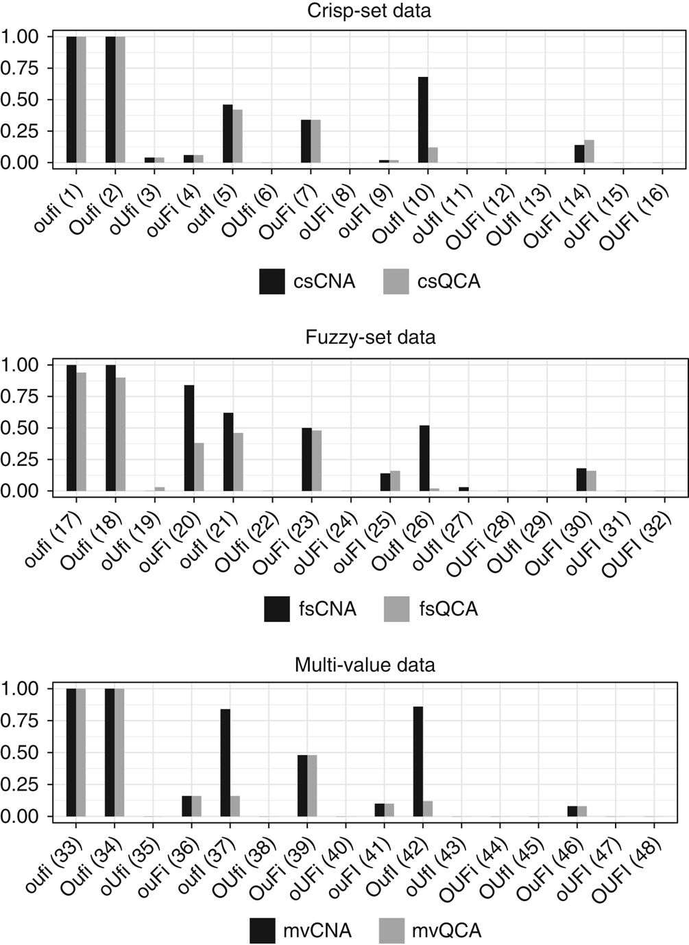
Figure 2 Completeness ratios for each test type, which are listed on the x-axis and numbered in correspondence with the replication script.
We end this discussion with some qualifications. The forms of data deficiencies analyzed here do not exhaust the space of possible deficiencies. For instance, all the data we simulated feature evenly distributed case frequencies, that is, different configurations are represented by roughly equally many cases. Of course, that is often not the case in real-life data. It is thus an open question how CNA and QCA fare and compare under biased case frequencies. Also, our test series sets consistency and coverage thresholds as well as diversity indices to constant values without exploring how the methods perform under variations of these values. Finally, although we only tested how CNA and QCA perform under various sorts of data deficiencies, we do not intend to suggest that data deficiencies are the only conceivable source of causal fallacies—apart from errors in the internal protocol of a method. There are a host of other sources for causal fallacies: for instance, errors in study designs, faulty background theories, or misapplications of a method. Our test series bracketed all of these problems. All findings reported above must hence be relativized to the particular sources of causal fallacies we chose to simulate.
Conclusion
This paper has generalized CNA, a CCM of causal data analysis, for multi-value variables and variables with continuous values from the unit interval that are interpreted as membership scores in fuzzy-sets. Moreover, it has shown in an extended series of benchmark tests that CNA performs both correctly and completely in ideal data scenarios and maintains reliable correctness ratios across a wide range of data deficiencies.
CNA differs from QCA, the currently dominant CCM, in numerous respects. First, CNA not only uncovers single-outcome structures but also structures with multiple outcomes. It is the only CCM custom-built to uncover the Boolean complexity dimension of sequentiality. Second, CNA builds causal models from the bottom up rather than from the top down. Thereby, it renders redundancy elimination (or minimization) itself redundant—which constitutes the algorithmic core of QCA. This reversal of the basic model building approach, on the one hand, allows CNA to abstain from erroneously causally interpreting irrelevant factors in cases of model overspecification and, on the other, permits CNA to directly apply one and the same algorithmic protocol to all data types, without a detour via truth tables. Third, CNA imposes authoritative consistency and coverage cutoffs on causal models (and all their elements), whereas QCA only uses a consistency threshold in truth table generation. In consequence, CNA is much more risk-averse than QCA when it comes to drawing causal inferences, which, in turn, yields that CNA maintains reasonably high correctness ratios even in scenarios featuring severe data deficiencies that cause QCA’s ratios to plummet. At the same time, we have seen that this inferential caution does not entail that CNA would fail to completely uncover data-generating structures where QCA succeeds in doing so.
Overall, the generalized version of CNA not only reliably uncovers all Boolean dimensions of causal structures from crisp-set, multi-value, and fuzzy-set data, but also has effective inbuilt controls that abandon an analysis that is too risky due to data deficiencies. In that light, CNA constitutes a powerful methodological alternative for researchers interested in the Boolean dimensions of causality.
Supplementary Materials
To view supplementary material for this article, please visit https://doi.org/10.1017/psrm.2018.45
Acknowledgement
The authors thank Alrik Thiem, Tim Haesebrouck, Simon Hug, and two anonymous PSRM referees for very helpful comments on previous versions of this article. Moreover, the authors have profited from discussions with audiences at the 5th International QCA Expert Workshop, Zürich 2017, and at the ECPR Joint Sessions Workshop “Configurational Thinking in Political Science: Theory, Methodology, and Empirical Application”, Nottingham 2017. Finally, the authors are grateful for generous support by the Swiss National Science Foundation (grant no. PP00P1_144736/1) and by the Bergen Research Foundation and University of Bergen (grant no. 811886).


