1 Quantities of Interest in Conjoint Experiments

Conjoint analysis serves two purposes. One is to assess causal effects. Another is preference description.Footnote ³ In causal inference, fully randomized conjoints provide a design and analytic approach that allows researchers to understand the causal effect of a given feature on overall support for a multidimensional object, averaging across other features of the object included in the design. Such inferences can be thought of as statements of the form: “shifting an immigrant’s country of origin from India to Poland increases favorability by X percentage points.” In descriptive inference, conjoints provide information about both (a) the absolute favorability of respondents toward objects with particular features or combinations of features and (b) the relative favorability of respondents toward an object with alternative combinations of features. Such inferences can be thought of as statements of the form “Polish immigrants are preferred by X% of respondents” or “Polish immigrants are more supported than Mexican immigrants, by X percentage points.” Thus, both causal and descriptive interpretations of conjoints are based on the distribution of preferences across profile features and differences in preferences across alternative feature combinations.

Analytically, a fully randomized conjoint design without constraints between profile features is simply a full-factorial experiment (with some cells possibly, albeit randomly, left unobserved). All quantities of interest relevant to the analysis of conjoint designs therefore derive from combinations of cell means, marginal means, and the grand mean, as in the traditional analysis of factorial experiments. In a forced-choice conjoint design, the grand mean is by definition 0.5 (i.e., 50% of all profiles shown are chosen and 50% are not chosen). Cell means are the mean outcome for each particular combination of feature levels. In the full-factorial design discussed by Hainmueller, Hopkins, and Yamamoto (Reference Hainmueller, Hopkins and Yamamoto2014) and now widely used in political science, many or perhaps most cell means are unobserved. For example, in their candidate choice experiment, there are $2\ast 6\ast 6\ast 6\ast 2\ast 6\ast 6\ast 6=\text{186,624}$ cell means but only 3,466 observations. About 98% of cell means are unobserved. While this would be problematic for attempting to infer pairwise comparisons between cells, conjoint analysts mostly focus on the marginal effects of each feature rather than more complex interactions. Supplementary Information Section A provides detailed notation and elaborations of the definitions of quantities of interest.

In fully randomized designs, the AMCEs are simply marginal effects of changing one feature level to another, all else constant. AMCEs therefore depend only upon marginal means: that is the column and row mean outcomes for each feature level averaging across all other features. A marginal mean describes the level of favorability toward profiles that have a particular feature level, ignoring all other features. For example, in the common forced-choice design with two alternatives, marginal means have a direct interpretation as probabilities. A marginal mean of 0 indicates that respondents select profiles with that feature level with probability $P(Y=1|X=x)=0$. While a marginal mean of 1 indicates that respondents select profiles with that feature level with probability $P(Y=1|X=x)=1$, where $Y$ is a binary outcome and $X$ is a vector of profile features.Footnote ⁴ With rating scale outcomes, marginal means can vary arbitrarily along the outcome scale used.

Because levels of features are randomly assigned, pairwise differences between two marginal means for a given feature (e.g., between candidates who are male versus female) have a direct causal interpretation. For fully randomized designs, the AMCE proposed by Hainmueller, Hopkins, and Yamamoto (Reference Hainmueller, Hopkins and Yamamoto2014) is equivalent to the average marginal effect of each feature level for a model where each feature is converted into a matrix of indicator variables with one level left out as a reference category. This is no different from any other regression context wherein one level of any categorical variable must be omitted from the design matrix in order to avoid perfect multicollinearity.Footnote ⁵ This close relationship between AMCEs and marginal means is visible in Figure 1 which presents a replication of the AMCE-based analysis of the Hainmueller et al. candidate experiment (left panel) and an analogous examination of the results using marginal means (right panel). Note, in particular, how marginal means convey information about the preferences of respondents for all feature levels while AMCEs definitionally restrict the AMCE for the reference category to zero (or undefined). For example, the AMCE for a candidate serving in the military is 0.09 (or 9 percentage points) increase in favorability, reflecting marginal means for serving and nonserving candidates of 0.46 and 0.54, respectively. Similarly, the zero effect size for candidate gender reflects identical marginal means for male and female candidates (0.50 in each case). AMCEs in fully randomized designs are simply differences between marginal means at each feature level and the marginal mean in the reference category, ignoring other features.

Figure 1. Replication of the Hainmueller, Hopkins, and Yamamoto (Reference Hainmueller, Hopkins and Yamamoto2014) candidate experiment using AMCEs and MMs.

The AMCE is often described as an estimate of the relative favorability of profiles with counterfactual levels of a feature. For example, Teele, Kalla, and Rosenbluth (Reference Teele, Kalla and Rosenbluth2018) summarize their conjoint on public support “female candidates are favored [over men] by 7.3 percentage points” (6). Similarly, Hainmueller, Hopkins, and Yamamoto (Reference Hainmueller, Hopkins and Yamamoto2014) describe some of the results of a conjoint on preferences toward political candidates:

These examples make clear that despite the causal inference potentially provided by the AMCE, the quantity of interest is frequently used to provide a characterization of a preference that has a distinctly descriptive flavor about the relative levels of support across profiles and also across subgroups of respondents. Indeed, this style of description is widespread in conjoint analyses. This use of conjoints to provide descriptive inferences about patterns of preferences is important because AMCEs are defined as relative quantities, requiring that patterns of preferences are expressed against a baseline, reference category for each conjoint feature. A positive AMCE is read as higher favorability, but it is only higher relative to whatever category that serves as the baseline. For example, in the Hainmueller, Hopkins, and Yamamoto candidate example, choosing a nonreligious candidate as a baseline and interpreting the resulting AMCEs means that the differences between other pairs of marginal means (e.g., evaluations of Mormon and Evangelical candidates) are not obvious. The negative direction, and the size, of the AMCEs for Mormon and Evangelical candidates would be different if the least-liked category of Mormons were the reference group. More trivially, Teele, Kalla, and Rosenbluth (Reference Teele, Kalla and Rosenbluth2018) describe their comparisons about public preferences for female candidates relative to male candidates, but could have also described patterns of equal size but opposite sign comparing preferences over male relative to female candidates. Supplementary Information Section B includes some additional illustrations of this point for interested readers.

2 Consequences of Arbitrary Reference Category Choice

How do researchers decide which of tens of thousands of possible experimental cells should be selected as the reference category? Examining recently published conjoint analyses, it appears that the choice of reference category is either arbitrary or based on substantive intuition about the meaning of feature levels. For example, Hainmueller, Hopkins, and Yamamoto (Reference Hainmueller, Hopkins and Yamamoto2014) choose female immigrants as a baseline in their immigration experiment, thus providing an estimate of the AMCE of being male, while Teele, Kalla, and Rosenbluth (Reference Teele, Kalla and Rosenbluth2018) choose male candidates as a baseline in their conjoint, thus providing an estimate of the AMCE of being female. The choice is seemingly innocuous. Sometimes, choices of reference category appear to be driven by substantive knowledge: on language skills of immigrants in their immigration experiment, Hainmueller, Hopkins, and Yamamoto (Reference Hainmueller, Hopkins and Yamamoto2014) choose fluency as a baseline; on the prior trips to the US feature, “never” is chosen as the baseline.

Table 1. Uses of subgroup analysis published in political science journals.

All articles in this table use subgroup conditional AMCEs to make inferences about differences in preferences between subgroups.

While seemingly arbitrary and innocuous, the choice of reference category can provide highly distorted descriptive interpretations of preferences among subgroups of respondents. This occurs when researchers examine conditional AMCEs, wherein AMCEs are calculated separately for subgroups of respondents and those conditional estimates are directly compared (Hainmueller, Hopkins, and Yamamoto Reference Hainmueller, Hopkins and Yamamoto2014, 13). Conditional AMCEs convey the causal effect of an experimental factor on overall favorability among the subgroup of interest. Consider, for example, a two-condition candidate choice experiment in which Democratic and Republican respondents are exposed to either a male or female candidate and opinions toward the candidate serve as the outcome. It is reasonable to imagine that effects of candidate sex might differ for the two groups and to therefore compare the size of treatment between the two groups. Perhaps Democrats are more responsive to candidate sex than are Republicans, making the causal effect larger for Democrats than Republicans. When conjoint analysts engage in subgroup comparisons, they are engaging in this kind of search for heterogeneous treatment effects across subgroups, but across a much larger number of experimental factors.

As Table 1 shows, discussions of conditional AMCEs in conjoint analyses often compare the size, and direction, of subgroup causal effects. Given the common practice of descriptively interpreting conjoint experimental results, such subgroup analyses seem perfectly intuitive. The set of subgroups listed in the last column of Table 1 contains some unsurprising covariates, such as partisanship, that are of obvious theoretical interest in almost any study of individual preferences. If interpreted as a difference in the size of the causal effect for two groups, such comparisons are perfectly consistent with more traditional experimental analysis and a perfectly acceptable interpretation of the conjoint results.

Yet, just as the analysis of full sample conjoint data is often descriptive in nature, it is also the case that conjoint analysts frequently interpret differences in conditional AMCEs descriptively rather than causally. For example, in one analysis, Hainmueller, Hopkins, and Yamamoto (Reference Hainmueller, Hopkins and Yamamoto2014) visually compare the pattern of AMCEs among high- and low-ethnocentrism respondents and interpret that “the patterns of support are generally similar for respondents irrespective of their level of ethnocentrism” (22). Ballard-Rosa, Martin, and Scheve (Reference Ballard-Rosa, Martin and Scheve2016) make similar comparisons in their tax policy conjoint: “While there are few strong differences in preferences for taxing the lower three income groups (the ‘hard work’ group has slightly lower elasticities for taxing the poor), there are strong differences in preferences for taxing the rich” (12). In the Bechtel and Scheve (Reference Bechtel and Scheve2013) conjoint on support for international climate change agreements in the United States, United Kingdom, Germany, and France, they summarize their results as “We find that individuals in all four countries largely agree on which dimensions are important and to what extent” (13765). In these examples, the differences between conditional AMCEs are used as a way of descriptively characterizing differences in preferences (i.e., levels of support) between the groups rather than differences in causal effects on preferences in the groups.

The selection of a reference category, while earlier an innocuous analytic decision, becomes substantially consequential for a descriptive reading of conditional AMCEs. Most obviously, using AMCEs descriptively prevents any description of the levels of favorability in the reference category. It can also lead to misinterpretations of patterns in preferences. AMCEs are relative, not absolute, statements about preferences. As such, there is simply no predictable connection between subgroup causal effects and the levels of underlying subgroup preferences. Yet, analysts and their readers frequently interpret differences in conditional AMCEs as differences in underlying preferences. AMCEs do provide insight into the descriptive variation in preferences within groups and across features, and conditional AMCEs do estimate the size of causal effects of features within groups. But AMCEs cannot provide direct insight into the pattern of preferences between groups because they do not provide information about absolute levels of favorability toward profiles with each feature (or combination of features).

This additional information matters. Consider again the simple two-condition experiment in which the effect of a male as opposed to female candidate, $x\in 0,1$, is compared across a single two-category covariate, $z\in 0,1$ such as Democratic or Republican self-identification. Subgroup regression equations to estimate effects for each group are

$$\begin{eqnarray}\displaystyle {\hat{y}} & = & \displaystyle \unicode[STIX]{x1D6FD}_{0}+\unicode[STIX]{x1D6FD}_{1}x+\unicode[STIX]{x1D716},\quad \forall z=0\nonumber\\ \displaystyle {\hat{y}} & = & \displaystyle \unicode[STIX]{x1D6FD}_{2}+\unicode[STIX]{x1D6FD}_{3}x+\unicode[STIX]{x1D716},\quad \forall z=1.\nonumber\end{eqnarray}$$

The effect of $x$ when $z=0$ is given by $\unicode[STIX]{x1D6FD}_{1}$. The effect of $x$ when $z=1$ is given by $\unicode[STIX]{x1D6FD}_{3}$. These are, in essence, the conditional AMCEs in a conjoint analysis. Yet, the difference in AMCEs ($\unicode[STIX]{x1D6FD}_{3}-\unicode[STIX]{x1D6FD}_{1}$) is not equal to the difference in preferences between the two groups, which is $\bar{y}_{z=1|x=1}-\bar{y}_{z=0|x=1}$ (estimated by $(\unicode[STIX]{x1D6FD}_{2}+\unicode[STIX]{x1D6FD}_{3})-(\unicode[STIX]{x1D6FD}_{0}+\unicode[STIX]{x1D6FD}_{1})$). The difference-in-AMCEs only equals the difference in preferences when $\unicode[STIX]{x1D6FD}_{2}\equiv \unicode[STIX]{x1D6FD}_{0}$. Yet, the standard AMCE-centric conjoint analysis does not present absolute favorability in the reference category. Similarity of conditional AMCEs only means similarity of the causal effect of the feature across groups and not similarity of preferences, unless preferences toward profiles with the reference category are equivalent in both groups. Given the reference category choice is typically arbitrary or driven by substantive knowledge of the levels, there is never any reason to expect that the reference category satisfies this equality requirement. When using a difference-in-AMCEs comparison to estimate a difference in preferences, the size and direction of the bias is determined by the size of the difference in preferences toward the reference category within each subgroup.

To draw this example out more fully, the upper panel of Figure 2 shows AMCEs for Teele, Kalla, and Rosenbluth’s candidate choice experiment for the full sample of respondents. The second panel shows full sample marginal means. Respondents’ preference for female candidates is very apparent in both forms of analysis in the upper two panels because the AMCE definitionally equals the difference in marginal means. But how do Republicans and Democrats differ in their preferences over male and female candidates? The third panel shows conditional AMCEs separately for Democratic and Republican voters, as provided in the original paper, and the lower panel shows the results using conditional marginal means for Democratic and Republican voters.Footnote ⁶ By requiring a reference category fixed to zero, the conditional AMCE results in the third panel suggest that there is a very large difference in favorability toward female candidates between Republican and Democratic respondents. In reality, however, the difference in these conditional AMCEs (0.089) reflects the true difference in favorability toward female candidates (difference: 0.045; Democrats: 0.537, Republicans: 0.492) plus the difference in favorability toward male candidates (difference: 0.045; Democrats: 0.463, Republicans: 0.508). Because Democrats and Republicans actually differ in their views of profiles containing the reference (male) category, AMCEs sum the true differences in preferences for a given feature level with the difference in preferences toward the reference category.Footnote ⁷

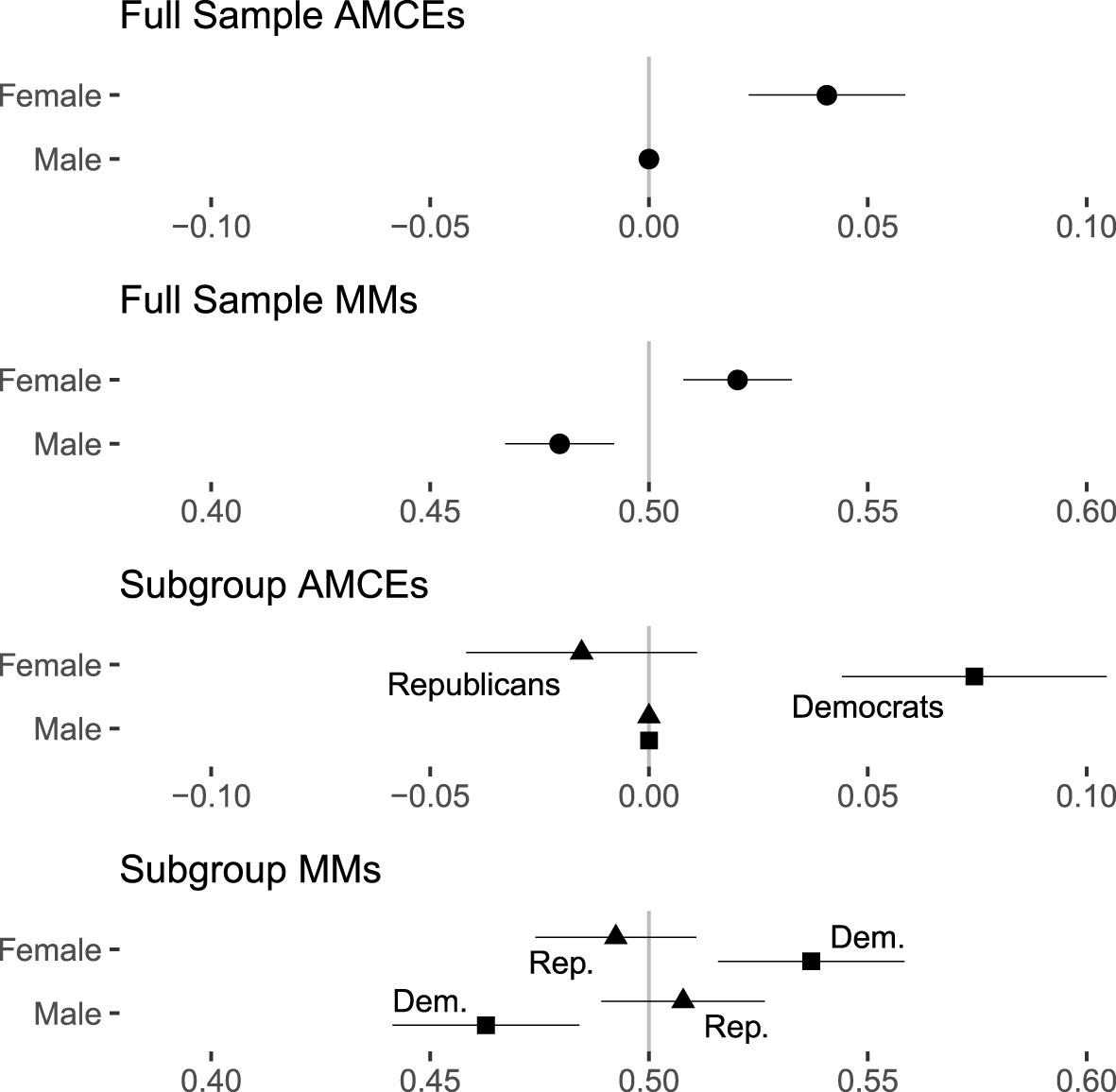
Figure 2. Replication of results for “candidate sex” feature from the Teele, Kalla, and Rosenbluth (Reference Teele, Kalla and Rosenbluth2018) candidate experiment using full sample AMCEs and marginal means (MMs) and subgroup AMCEs and MMs for Democrats and Republicans.

Visual or numerical similarity of subgroup AMCEs is therefore an analytical artifact, not an accurate statement of the similarity of patterns of preferences. We can see this bias in a reanalysis of Bechtel and Scheve’s four-country climate change agreement experiment. Figure 3 shows an analysis for the feature capturing the monthly household cost for a potential international climate agreement. This replicates a portion of their results which compare high- and low-environmentalism respondents pooled across countries (Bechtel and Scheve Reference Bechtel and Scheve2013, 13767 figure 4). The original analysis has conditional AMCEs for the two subgroups with 28 Euro per month as the reference category. Conditional AMCEs for both groups are presented as negative with conditional AMCEs for low-environmentalism respondents being more negative than the conditional AMCEs for high-environmentalism respondents at every feature level. This implies positive differences in favorability toward each monthly cost between high- and low-environmentalism respondents. Figure 3 presents the implied difference-in-AMCEs from the original analysis as black circles, demonstrating the substantial and positive apparent differences between the two groups. For example, the difference-in-AMCEs for the 56 Euro per month level (incorrectly) implies that high-environmentalism respondents are more favorable toward a 56 Euro per month household cost of an agreement than are low-environmentalism respondents. Yet, the opposite is actually true: high-environmentalism respondents are less favorable toward this option than low-environmentalism respondents. By using the 28 Euro per month level as the reference category, the original analysis implies that preferences are identical between the two groups when in reality, high-environmentalism respondents are much less favorable toward a 28 Euro per month cost than low-environmentalism respondents. The black diamonds in Figure 3 show these true differences in favorability as marginal means for the two groups.

Figure 3. True difference in favorability and implied preference differences between high- and low-environmentalism respondents for “monthly cost” feature from the Bechtel and Scheve (Reference Bechtel and Scheve2013) climate agreement experiment for each possible reference category.

Furthermore, the gray dots in Figure 3 represent the alternative differences-in-AMCEs that could have been generated from alternative choices of reference category using the same data. Not only is it possible for reference category choice to significantly color the apparent size of differences between subgroup, that choice can also impact the direction and statistical significance of subgroup differences. An analyst could easily choose a reference category that presents the differences between these two groups as large and positive, small and positive, small and negative, large and negative, or negligible. The original analysis (again, black circles) happens to show large and positive differences between the groups.

It is worth highlighting two further features in Figure 3. First, the alternative differences-in-AMCEs estimates vary mechanically around the difference in marginal means, as the reference category varies. The difference between marginal means for two groups are always fixed in the data, so the differencing of subgroup AMCEs is merely an exercise that is centering those differences at arbitrary points along the range of observed differences in marginal means. Second, and more practically, because there is no category for which the preferences of the two subgroups in this example are identical, no choice of reference category would have led to inferences from differences-in-AMCEs that accurately reflect the underlying difference in preferences. Even in the 84 Euro per month level, the difference between the two groups is slightly positive. Were there a category for which subgroup preferences were exactly equal, then we could choose that as the reference category and interpret differences-in-AMCEs as differences in preferences. But there is never any guarantee that such a reference category exists. Thus, there is no way to use conditional AMCEs or differences between those conditional AMCEs to convey the underlying similarity or differences in preferences across sample subgroups.

3 Improved Subgroup Analyses in Conjoint Designs

Researchers and consumers of conjoints interested in describing levels of respondent favorability toward profiles with varying features can avoid the inferential errors that accompany conditional AMCEs by focusing attention on (subgroup) marginal means, differences between subgroup marginal means to infer subgroup differences in preferences toward particular features, and omnibus nested model comparisons to infer subgroup differences across many features. To demonstrate each of these three techniques, we provide a complete example based on Hainmueller, Hopkins, and Yamamoto’s analysis of their immigration conjoint by respondent ethnocentrism, which finds that “the patterns of support are generally similar for respondents irrespective of their level of ethnocentrism” (Hainmueller, Hopkins, and Yamamoto Reference Hainmueller, Hopkins and Yamamoto2014, 22). First, we show how different reference categories could have led to distinctly different conditional AMCEs and, therefore, interpretations of subgroup preference similarity. Second, we show how differences in marginal means clearly convey the similarity of these two subgroups without any sensitivity to reference category. Finally, we show how tested model comparisons would have provided Hainmueller, Hopkins, and Yamamoto with a statistic test of the claimed similarity in levels of support between these two respondent subgroups.

Figure 4. Comparison of AMCEs for low- and high-ethnocentrism respondents using two alternative reference category choices for three features from Hainmueller et al.’s (Reference Hainmueller, Hopkins and Yamamoto2014) immigration experiment.

To begin with, consider the left and right facets of Figure 4, which shows estimated subgroup AMCEs for three features from the immigration study. In panel A (left), all features are configured so that the reference category is the one with the largest difference in levels of support between the two subgroups, thus distorting the size of differences at all other levels. In panel B (right), all features are configured so that the reference category is the one with the smallest difference in preferences between the two subgroups.

Panel A gives the impression that there are significant differences in preferences between high- and low-ethnocentrism respondents toward immigrants from different countries of origin, with different careers, and with different educational attainments because the reference category choice cascades the difference in reference category favorability into AMCEs for all other feature levels. By contrast, Panel B gives the impression that these differences are negligible. The experimental data and analytic approach in the two portrayals is identical; the only difference is the choice of reference category. Given what we have shown about the relationship between differences in conditional AMCEs and differences in conditional marginal means, Panel B is a more “truthful” visualization, which Cairo (Reference Cairo2016) uses to mean avoidance of self-deception in the presentation of data, and a more “functional” visualization, by which Cairo means choosing graphics based on how they will be interpreted by the visualization’s consumers. The differences between subgroup AMCEs there more accurately convey differences in underlying preferences because the reference categories used in Panel B are the most similar between the two groups.

Figure 5. Differences in conditional marginal means, by ethnocentrism, for three features from Hainmueller et al.’s (Reference Hainmueller, Hopkins and Yamamoto2014) immigration experiment.

Next, making a comparison of levels of favorability toward different types of immigrants without using AMCEs would have been even more truthful. Figure 5 directly shows the comparison of preferences as differences in subgroup marginal means between the two groups for these three features, with 95% confidence intervals for the difference.Footnote ⁸ The two groups indeed have similar preferences, something that would have happened to be clear had the conditional AMCEs in the right panel of Figure 4 been presented but that would have been far less obvious were the conditional AMCEs in the left panel of that figure were presented. The pairwise difference in means tests would provide formal procedures for testing the statistical significance of these differences.

Yet, finally, the similarity of subgroup preferences in conjoints is often characterized in an omnibus fashion, as in the quote from Hainmueller, Hopkins, and Yamamoto (Reference Hainmueller, Hopkins and Yamamoto2014) describing “patterns of support.” An appropriate test in such cases is one that evaluates whether a model of support that accounts for group differences better fits the data than a model of support with only conjoint features as predictors. This type of test is known as a “nested model comparison” which compares the fit of a “restricted” regression (the restriction being that interactions between features and a subgroup identifier are held to be zero) nested within an “unrestricted” regression that allows for arbitrary interactions between conjoint features and the subgroup identifier. Formally, a nested model comparison provides an F-test of the null hypothesis that all interaction terms are equal to zero.Footnote ⁹

To make this concrete, for a feature with four levels (one treated as a reference category), the first (restricted) equation would be the following:

(1)$$\begin{eqnarray}Y=\unicode[STIX]{x1D6FD}_{0}+\unicode[STIX]{x1D6FD}_{1}\mathit{Level}_{2}+\unicode[STIX]{x1D6FD}_{2}\mathit{Level}_{3}+\unicode[STIX]{x1D6FD}_{3}\mathit{Level}_{4}+u.\end{eqnarray}$$

The second (unrestricted) equation would allow for interactions between feature levels and the subgroup identifier:

(2)$$\begin{eqnarray}\displaystyle Y & = & \displaystyle \unicode[STIX]{x1D6FD}_{0}+\unicode[STIX]{x1D6FD}_{1}\mathit{Level}_{2}+\unicode[STIX]{x1D6FD}_{2}\mathit{Level}_{3}+\unicode[STIX]{x1D6FD}_{3}\mathit{Level}_{4}+\unicode[STIX]{x1D6FD}_{4}\mathit{Group}\nonumber\\ \displaystyle & & \displaystyle +\,\unicode[STIX]{x1D6FD}_{5}\mathit{Level}_{2}\ast \mathit{Group}+\unicode[STIX]{x1D6FD}_{6}\mathit{Level}_{3}\ast \mathit{Group}+\unicode[STIX]{x1D6FD}_{7}\mathit{Level}_{4}\ast \mathit{Group}+u.\end{eqnarray}$$

While Equation (1) imposes the constraint that $\unicode[STIX]{x1D6FD}_{4}=\unicode[STIX]{x1D6FD}_{5}=\unicode[STIX]{x1D6FD}_{6}=\unicode[STIX]{x1D6FD}_{7}=0$, Equation (2) allows for subgroup differences in favorability. Testing this null entails computing an F-statistic comparing the fit of each equation:

(3)$$\begin{eqnarray}F={\displaystyle \frac{\frac{\mathit{SSR}_{\mathit{Restricted}}-\mathit{SSR}_{\mathit{Unrestricted}}}{r}}{\frac{\mathit{SSR}_{\mathit{Unrestricted}}}{n-k-1}}},\end{eqnarray}$$

where $\mathit{SSR}_{\mathit{Restricted}}$ is the sum of squared residuals for Equation (1), $\mathit{SSR}_{\mathit{Unrestricted}}$ is the sum of squared residuals for Equation (2), $r$ is the number of restrictions (in the above example, 4), $n$ is the number of cases, and $k$ is the number of feature levels in the unrestricted model.Footnote ¹⁰

For the education feature, the resulting F-test for the model comparison in this case again gives us little reason to believe that there are subgroup differences: $\text{F}(7,\text{11,493})=0.68$, $p\leqslant 0.69$. We could repeat such pairwise comparisons or omnibus comparisons for each feature in the design—for country of origin ($\text{F}(10,\text{11,490})=1.56$, $p\leqslant 0.11$) or job ($\text{F}(11,\text{11,489})=0.87$, $p\leqslant 0.56$)— or for all features as a whole ($\text{F}(98,\text{11,402})=1.16$, $p\leqslant 0.14$).

This visual display in Figure 5 and these statistical tests make clear what could not be directly inferred from conditional AMCEs alone; there are indeed no sizeable and only a few statistically apparent differences in preferences between the two groups.

This kind of nested model comparison test can also be used to assess heterogeneity across conjoint features (see also Egami and Imai Reference Egami and Imai2018). For example, Teele, Kalla, and Rosenbluth (Reference Teele, Kalla and Rosenbluth2018) report just such a test for how effects of features other than candidate sex may differ between male and female candidates, finding no such heterogeneity (8–9). Fortunately, the original analysis accurately detected an absence of subgroup differences; yet, a subtly different set of analytic decisions about reference categories (as shown in Figure 4) could have led to quite different inferences. As an example, Bechtel and Scheve (Reference Bechtel and Scheve2013) argue that their conjoint results show that “individuals in all four countries [Germany, France, United States, United Kingdom] largely agree on which dimensions are important and to what extent” (Bechtel and Scheve Reference Bechtel and Scheve2013, 13765), but a nested model comparison shows that the countries do differ in their preferences $\text{F}(54,\text{67,982})=3.72$, $p\leqslant 0.00$. This cross-country variation is largely driven by differences in sensitivity to monthly household costs feature, $\text{F}(15,\text{67,995})=3.80$, $p\leqslant 0.00$, with the United Kingdom and United States being more cost sensitive than Germany and France. Visual comparisons of conditional AMCEs can sometimes provide accurate insights into subgroup differences in preferences (as in the Hainmueller, Hopkins, and Yamamoto case), but ultimately there is no guarantee that they do in any particular analysis.