3.1 Kernels as nonlinear feature mappings

Prediction techniques such as support vector machines (SVMs) learn decision surfaces that correspond to hyper-planes in the original feature space by computing inner products between input examples; consequently, they are inherently linear and cannot discover nonlinear patterns in data. A possible solution is to use a mapping $$ \phi :x \in {\Bbb R}^n \mapsto \phi (x) \in F \subseteq {\Bbb R}^N $$ such that nonlinear relations in the original space become linearly separable in the target projection space, enabling the SVM to correctly separate the data by computing inner products $$ \langle \phi (x_i ),\phi (x_j )\rangle $$ in the new feature space. However, such projections can be computationally intense. Kernel functions are a class of functions that allow to compute $$ \langle \phi (x_i ),\phi (x_j )\rangle $$ without explicitly accessing the input representation in the projection space. Formally, given a feature space X and a mapping ϕ from X to F, a kernel κ is any function satisfying

(1) $$ \kappa (x_i ,x_j ) = \langle \phi (x_i ),\phi (x_j )\rangle \quad \forall x_i ,x_j \in X $$

An important generalization result is the Mercer Theorem (Shawe-Taylor and Cristianini Reference Shawe-Taylor and Cristianini2004), stating that for any symmetric positive semi-definite function κ there exists a mapping ϕ such that 1 is satisfied. Hence, kernels include a broad class of functions (Shawe-Taylor and Cristianini Reference Shawe-Taylor and Cristianini2004). Research community has been exploring kernel methods for decades and a wide variety of kernel paradigms have been proposed. In the following subsections, we will illustrate advancements in TKs, as they are well suited to encode formalisms, such as dependency graphs or grammatical trees, traditionally exploited in the linguistics communities.

3.2 Semantic kernels

Learning to solve NLP tasks usually involves the acquisition of decision models based on complex semantic and syntactic phenomena. For instance, in Paraphrase Detection, verifying whether two sentences are valid paraphrases involves rewriting rules in which the syntax plays a fundamental role. In Question Answering, the syntactic information is crucial, as largely demonstrated in Croce, Moschitti, and Basili (Reference Croce, Moschitti and Basili2011). Similar needs are applicable to the Semantic Role Labeling task that consists in the automatic discovery of linguistic predicates (together with their corresponding arguments) in texts. A natural approach to such problems is to apply Kernel methods (Robert Müller, Mika, Rätsch, Tsuda, and Schölkopf Reference Robert Müller, Mika, Rätsch, Tsuda and Schölkopf2001; Shawe-Taylor and Cristianini Reference Shawe-Taylor and Cristianini2004) that have been traditionally proposed to decouple similarity metrics and learning algorithms in order to alleviate the impact of feature engineering in inductive processes. Kernels may directly operate on complex structures and then be used in combination with linear learning algorithms, such as SVMs (Vapnik Reference Vapnik1998). Sequence (Cancedda, Gaussier, Goutte, and Renders Reference Cancedda, Gaussier, Goutte and Renders2003) or TKs (Collins and Duffy Reference Collins and Duffy2001) are of particular interest as the feature space they capture reflects linguistic patterns. A sentence can be represented as a parse tree that expresses the grammatical relations implied by s: parse trees are extracted by using the Stanford Parser (Manning, Surdeanu, Bauer, Finkel, Bethard, and Mc-Closky Reference Manning, Surdeanu, Bauer, Finkel, Bethard and McClosky2014). TKs (Collins and Duffy Reference Collins and Duffy2001) can be employed to directly operate on such parse trees, evaluating the tree fragments shared by the input trees. This operation corresponds to a dot product in the implicit feature space of all possible tree fragments. Whenever the dot product is available in the implicit feature space, kernel-based learning algorithms, such as SVMs (Cortes and Vapnik Reference Cortes and Vapnik1995), can operate in order to automatically generate robust prediction models. TKs thus allow estimating the similarity among texts, directly from sentence syntactic structures, that can be represented by parse trees. The underlying idea is that the similarity between two trees T ₁ and T ₂ can be derived from the number of shared tree fragments. Let the set $$ {\cal T} = \{ t_1 ,t_2 , \ldots ,t_{|{\cal T}|} \} $$ be the space of all the possible substructures and $$ \chi _i (n_2 ) $$ be an indicator function that is equal to 1 if the target t_i is rooted at the node n ₂ and 0 otherwise. A TK function over T ₁ and T ₂ is defined as follows: $$ TK(T_1 ,T_2 ) = \sum\nolimits_{n_1 \in N_{T_1 } } \sum\nolimits_{n_2 \in N_{T_2 } } \Delta (n_1 ,n_2 ) $$ where N _{T 1} and N _{T 2} are the sets of nodes of T ₁ and T ₂, respectively, and $$ \Delta (n_1 ,n_2 ) = \sum\nolimits_{k = 1}^{|{\cal T}|} \chi _k (n_1 )\chi _k (n_2 ) $$ which computes the number of common fragments between trees rooted at nodes n ₁ and n ₂. The feature space generated by the structural kernels obviously depends on the input structures. Note that different tree representations embody different linguistic theories and may produce more or less effective syntactic/semantic feature spaces for a given task.

Many available linguistic resources are enriched with formalisms dictated by Dependency grammars and produce a significantly different representation as exemplified in Figure 1. Since TKs are not tailored to model the labeled edges that are typical of dependency graphs, these latter are rewritten into explicit hierarchical representations. Different rewriting strategies are possible, as discussed in Croce, Moschitti, and Basili (Reference Croce, Moschitti and Basili2011): a representation that is shown to be effective in several tasks is the grammatical relation centered tree (GRCT) illustrated in Figure 2: the PoS-Tags are children of grammatical function nodes and direct ancestors of their associated lexical items. Another possible representation is the Lexical only centered tree (LOCT) shown in Figure 3, which contains only lexical nodes and the edges reflect some dependency relations.

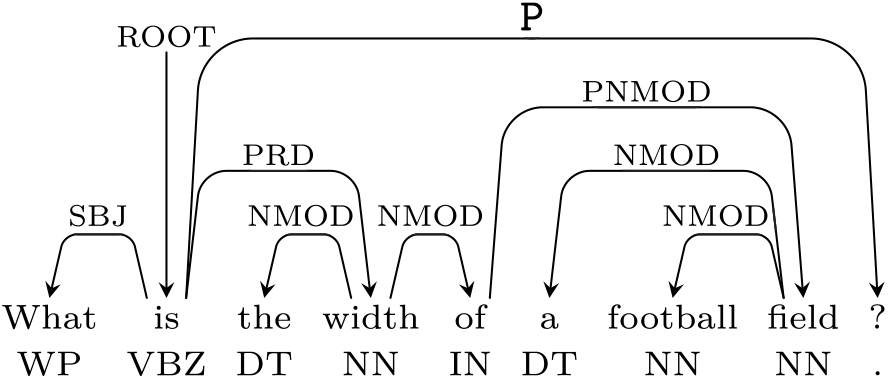
Figure 1: Dependency parse tree of “What is the width of a football field?”.

Figure 2: Grammatical Relation Centered Tree (GRCT) of “What is the width of a football field?”.

Figure 3: Lexical only centered tree (LOCT) of “ What is the width of a football field?”.

Different TKs can be defined according to the types of tree fragments considered in the evaluation of the matching structures. Subset of trees are exploited by the subset tree kernel (Collins and Duffy Reference Collins and Duffy2001), which is usually referred to as syntactic tree kernel (STK); they are more general structures since their leaves can be also nonterminal symbols. The subset trees satisfy the constraint that grammatical rules cannot be broken and every tree exhaustively represents a CFG rule. Partial tree kernel (PTK; Moschitti Reference Moschitti2006) relaxes this constraint considering partial trees, that is, fragments generated by the application of partial production rules (e.g., sequences of nonterminal nodes with gaps). The strict constraint imposed by the STK may be problematic especially when the training dataset is small and only few syntactic tree configurations can be observed. Overcoming this limitation, the PTK usually leads to higher accuracy, as shown by Moschitti (Reference Moschitti2006).

Capitalizing lexical semantic information in convolution kernels

The TKs introduced in previous section perform a hard match between nodes when comparing two substructures. In NLP tasks, when nodes are words, this strict requirement reflects in a too strict lexical constraint that poorly reflects semantic phenomena, such as the synonymy of different words or the polysemy of a lexical entry. To overcome this limitation, we adopt Distributional models of Lexical Semantics (Schütze Reference Schütze1993; Sahlgren Reference Sahlgren2006; Padó and Lapata Reference Padó and Lapata2007) to generalize the meaning of individual words by replacing them with geometrical representations (also called Word Embeddings) that are automatically derived from the analysis of large-scale corpora (Mikolov et al. Reference Mikolov, Chen, Corrado and Dean2013). These representations are based on the idea that words occurring in the same contexts tend to have similar meaning: the adopted distributional models generate vectors that are similar when the associated words exhibit a similar usage in large-scale document collections. Under this perspective, the distance between vectors reflects semantic relations between the represented words, such as paradigmatic relations, for example, quasi-synonymy.^{Footnote a} These word spaces allow to define meaningful soft matching between lexical nodes, in terms of the distance between their representative vectors. As a result, it is possible to obtain more informative kernel functions, which are able to capture syntactic and semantic phenomena through grammatical and lexical constraints. Moreover, the supervised setting of a learning algorithm (such as SVM), operating over the resulting kernel, is augmented with the word representations generated by the unsupervised distributional methods, thus characterizing a cost-effective semi-supervised paradigm.

The smoothed partial tree kernel (SPTK) described in Croce et al. (Reference Croce, Moschitti and Basili2011) exploits this idea extending the PTK formulation with a similarity function σ between nodes:

(2) $$\eqalign{ \Delta _{SPTK} (n_1 ,n_2 ) = & \mu \lambda \sigma (n_1 ,n_2 ),\quad {\rm{if}}\,n_1 \,{\rm{and}}\,n_2 \,{\rm{are}}\,{\rm{leaves}} \cr \Delta _{SPTK} (n_1 ,n_2 ) = & \mu \sigma (n_1 ,n_2 )\left( {\lambda ^2 + \sum\limits_{\vec I_1 ,\vec I_2 :l(\vec I_1 ) = l(\vec I_2 )} {\lambda ^{d(\vec I_1 ) + d(\vec I_2 )} \prod\limits_{k = 1}^{l(\vec I_1 )} {\Delta _{SPTK} \left( {c_{n_1 } \left( {i_k^1 } \right),c_{n_2 } \left( {i_k^2 } \right)} \right)} } } \right) \cr} $$

In the SPTK formulation, the similarity function σ(n ₁, n ₂) between two nodes n ₁ and n ₂ can be defined as follows:

• • if n ₁ and n ₂ are both lexical nodes, then $$ \sigma (n_1 ,n_2 ) = \sigma _{LEX} (n_1 ,n_2 ) = \tau {{\vec v_{n_1 } \cdot \vec v_{n_2 } } \over {\left\| {\vec v_{n_1 } } \right\|\left\| {\vec v_{n_2 } } \right\|}} $$. It is the cosine similarity between the word vectors $$ \vec v_{n_1 } $$ and $$ \vec v_{n_2 } $$ associated with the labels of n ₁ and n ₂, respectively. τ is called terminal factor and weighs the contribution of the lexical similarity to the overall kernel computation.

• • else if n ₁ and n ₂ are nodes sharing the same label, then σ(n ₁, n ₂) = 1.

• • else σ(n ₁, n ₂) = 0.

The decay factors λ and μ are responsible for penalizing large child subsequences (that can include gaps) and partial sub-trees that are deeper in the structure, respectively.

Dealing with compositionality in TKs

The main limitations of the SPTK are that (i) lexical semantic information only relies on the vector metrics applied to the leaves in a context-free fashion and (ii) the semantic compositions between words are neglected in the kernel computation that only depends on their grammatical labels.

In Annesi, Croce, and Basili (Reference Annesi, Croce and Basili2014), a solution for overcoming these issues is proposed. The pursued idea is that the semantics of a specific word depends on its context. For example, in the sentence, “What instrument does Hendrix play?”, the role of the word instrument is fully captured if its composition with the verb play is taken into account. Such combination of lexical semantic information can be directly expressed into the tree structures, as shown in Figure 4. The resulting representation is a compositional extension of a GRCT structure, where the original label d_n of grammatical function nodes n (i.e., dependency relations in the tree) is augmented by also denoting their corresponding head/modifier pairs (h_n, m_n).

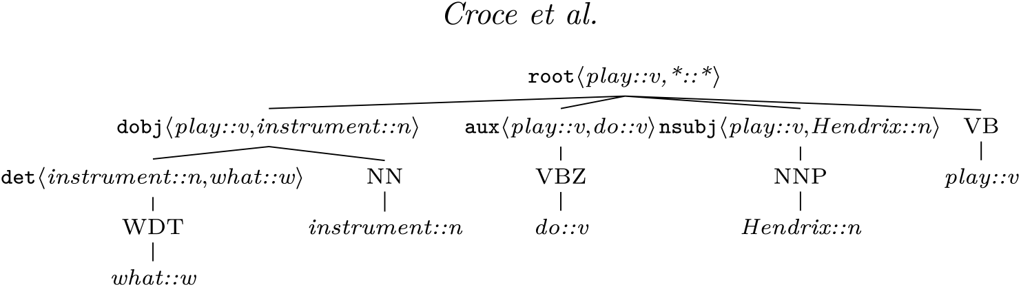
Figure 4: Compositional grammatical relation centered tree (CGRCT) of the sentence “ What instrument does Hendrix play?”.

In CGRCTs, a (sub)tree rooted at dependency nodes can be used to provide a contribution to the kernel that is a function of the composition of vectors, $$ \vec h $$ and $$ \vec m $$, expressing the lexical semantics of the head h and modifier m, respectively. Several algebraic functions have been proposed in Annesi et al. (Reference Annesi, Croce and Basili2014) to compose the vectors of h=l^h::pos^h and m=l^m::pos^m into a vector $$ \vec c^{h,m} $$ representing the head modifier pair c = 〈l^h::pos^h,l^m::pos^m〉, in line with the research on Compositional Distributional Semantics (e.g., Mitchell and Lapata Reference Mitchell and Lapata2010). In this work, we investigated the additive function (according to the notation proposed in Mitchell and Lapata Reference Mitchell and Lapata2010) that assigns to a head/modifier pair c the vector resulting from the linear combination of the vectors representing the head and the modifier, that is, $$ \vec c^{h,m} = \alpha \vec h + \beta \vec m $$. Although this composition method is very simple and efficient, it actually produces very effective kernel functions, as demonstrated in Annesi et al. (Reference Annesi, Croce and Basili2014) and Filice et al. (Reference Filice, Castellucci, Croce and Basili2015). According to the CGRCT structures, Annesi et al. (Reference Annesi, Croce and Basili2014) define the compositionally smoothed partial tree kernel (CSPTK). The core novelty of the CSPTK is the compositionally enriched estimation of the function σ. The function σ can be applied to lexical nodes, to POS tag nodes as well as to augmented dependency nodes. In the algorithm the three cases are defined. For simple lexical nodes, σ consists of a lexical kernel σ _LEX, such as the cosine similarity between word vectors (sharing the same POS-tag): this is equivalent to Croce et al. (Reference Croce, Moschitti and Basili2011). For POS nodes σ consists of the identity function that is 1 only when the same POS is matched and it is 0 elsewhere.

The novelty of CSPTK corresponds to the compositional treatment of two dependency nodes, n ₁ = 〈d ₁, h ₁, m ₁ and n ₂ = 〈d ₂, h ₂, m ₂. The similarity function σ in this case corresponds to a compositional function σ _Comp between the two nodes σ _Comp is not null only when the two nodes exhibit the same dependency relation, that is, d = d ₁ = d ₂, so that also the respective heads and modifiers share the same POS labels: this allows to exploit, case by case, the suitable contextual meaning of polysemous words, e.g. bank. In all these cases a compositional metric is applied over the two involved (h_i, m_i) compounds. In the simple case, the cosine similarity between the two vectors $$ \vec c_i ^{h_i ,m_i } = \alpha \vec h_i + \beta \vec m_i $$, i=1,2, is applied. Other metrics correspond to more complex compositions $$ \Psi ((\vec h_1 ,\vec m_1 ),(\vec h_2 ,\vec m_2 )) $$ that account for linear algebra operators among the four vectors.

3.3 Approximating kernel spaces through the Nyström method

Given an input training dataset $$ {\cal D}$$ of objects o_i, i = 1 … N, a kernel K(o_i, o_j) is a similarity function over $${\cal D}^2$$that corresponds to a dot product in the implicit kernel space, that is, $$ K(o_i ,o_j ) = \Phi (o_i ) \cdot \Phi (o_j ) $$. The advantage of kernels is that the projection function $$\Phi (o) = \vec x \in {\Bbb R} ^n$$ is never explicitly computed (Shawe-Taylor and Cristianini Reference Shawe-Taylor and Cristianini2004). In fact, this operation may be prohibitive when the dimensionality n of the underlying kernel space is extremely large, as for TKs (Collins and Duffy Reference Collins and Duffy2001). Kernel functions are used by learning algorithms, such as SVM, to operate only implicitly on instances in the kernel space, by never accessing their explicit definition. Let us apply the projection function Φ over all examples o_i from $${\cal D}$$ to derive representations, $$ \vec x_i $$ denoting the th row of the matrix X. The Gram matrix can always be computed as G = XX^⊤, with each single element corresponding to $$ {\bf{G}}_{ij} = \Phi (o_i )\Phi (o_j ) = K(o_i ,o_j ) $$. The aim of the Nyström method (Drineas and Mahoney Reference Drineas and Mahoney2005) is to derive a new low-dimensional embedding $$ {\tilde {\vec x}} $$ in a l-dimensional space, with l ≪ n so that $$ {\bf{\tilde G}} = {\bf{\tilde X\tilde X}}^{\rm T} $$ and $$ {\bf{\tilde G}} \approx {\bf{G}} $$. This is obtained by generating an approximation $${\bf{\tilde G}}$$ of G using a subset of l columns of the Gram matrix, that is, the kernel evaluations between all the objects $$ \in {\cal D} $$ and a selection of a subset $$ L \subset {\cal D} $$ of the available examples, called landmarks. Suppose we randomly sample l columns of G, and let $$ {\bf{C}} \in ^{N \times l} $$ be the matrix of these sampled columns. Then, we can rearrange the columns and rows of G and define X = [X₁ X₂] such that:

$$ {\bf{G}} = {\bf{XX}}^{\rm T} = \left[ {\matrix{ {\bf{W}} & {{\bf{X}}_1^{\rm T} {\bf{X}}_2 } \cr {{\bf{X}}_2^{\rm T} {\bf{X}}_1 } & {{\bf{X}}_2^{\rm T} {\bf{X}}_2 } \cr } } \right]\quad {\rm{and}}\quad {\bf{C}} = \left[ {\matrix{ {\bf{W}} \cr {{\bf{X}}_2^{\rm T} {\bf{X}}_1 } \cr } } \right] $$

where $$ {\bf{W}} = {\bf{X}}_1^{\rm T} {\bf{X}}_1 $$, that is, the subset of G that contains only landmarks and C kernel evaluations between landmarks and the remaining examples. The Nyström approximation can be defined as

(3) $$ {\bf{G}} \approx {\bf{\tilde G}} = {\bf{CW}}^{{\dag} {\bf{C}}^{\rm T}} $$

where W^† denotes the Moore–Penrose inverse of W. The singular value decomposition (SVD) is used to obtain W^† as follows. First, W is decomposed so that W = USV^T, where U and V are both orthogonal matrices, and S is a diagonal matrix containing the (nonzero) singular values of W on its diagonal. Since W is symmetric and positive definite, it holds that W =USU^T. Then, $${\bf{W}}^{\dag = {\bf{US}}}^{ - 1} {\bf{U}}^{\rm T} = {\bf{US}}^{ - {1 \over 2}} {\bf{S}}^{ - {1 \over 2}} {\bf{U}}^{\rm T}$$ and Equation (3) can be rewritten as

(4) $${\bf{G}} \approx {\bf{\tilde G}} = {\bf{CUS}}^{ - {1 \over 2}} {\bf{S}}^{ - {1 \over 2}} {\bf{U}}^{\rm T} {\bf{C}}^{\rm T} = ({\bf{CUS}}^{ - {1 \over 2}} )({\bf{CUS}}^{ - {1 \over 2}} )^{\rm T} = {\bf{\tilde X\tilde X}}^{\rm T} $$

which explicitates the desired approximation of G in terms of the described decomposition. Given an input example $$o \in {\cal D}$$, a new low-dimensional representation $$\tilde {\vec x}$$can be thus determined by considering the corresponding item of C as

(5) $$\tilde {\vec x} = {\vec c}{\bf{\,US}}^{ - {1 \over 2}} $$

where $$\vec c $$ is the vector whose jth individual component contains the evaluation of the kernel function between o and the landmark $$o_j \in L$$. Therefore, the method produces l-dimensional vectors.

Figure 5: Kernel-based deep architecture.

4.1 Kernel-based deep architectures

As discussed in Section 3.3, the Nyström representation $$ \tilde {\vec x} $$ of any input example o is linear and can be adopted to feed a neural network architecture. We assume a labeled dataset $${\cal L} = \{ (o,y)\,|\,o\in {\cal D}, \,\,y \in Y\}$$ being available, where o refers to a generic instance and y is its associated class. In this section, we define a multilayer perceptron (MLP) architecture, with a specific Nyström layer based on the Nyström embeddings of Equation (5). We will refer to this architecture, shown in Figure 5, as KDA. KDA has an input layer, a Nyström layer, a possibly empty sequence of nonlinear hidden layers and a final classification layer, which produces the output.

The input layer corresponds to the input vector $${\vec c}$$, that is, the row of the C matrix associated with an example o. Note that, for adopting the KDA, the values of the C matrix should be all available. In the training stage, these values are in general cached. During the classification stage, the $${\vec c}$$ vector corresponding to an example o is directly computed by l kernel computations between and each of the l landmarks.

The input layer is mapped to the Nyström layer, through the projection in Equation (5). Note that the embedding provides also the proper weights, defined by $$ {\bf{US}}^{ - {1 \over 2}}$$, so that the mapping can be expressed through the Nyström matrix $$ {\bf{H}}_{Ny} = {\bf{US}}^{ - {1 \over 2}} $$: it corresponds to a pretrained stage derived through SVD, as discussed in Section 3.3. Equation (5) provides a static definition for H_Ny whose weights can be left invariant during the neural network training. However, the values of H_Ny can be made available for the standard back-propagation adjustments applied for training. Formally, the low-dimensional embedding of an input example, o, is $$\tilde {\vec x} = {\vec c}{\,\bf{H}}_{Ny} = {\vec c}{\,\bf{US}}^{ - {1 \over 2}} $$.

The resulting outcome $$ \tilde {\vec x} $$ is the input to one or more nonlinear hidden layers. Each th hidden layer is realized through a matrix $$ {\bf{H}}_t \in {\Bbb R}^{h_{t - 1} \times h_t } $$ and a bias vector $$ \vec b_t \in {\Bbb R}^{1 \times h_t } $$, whereas h_t denotes the desired hidden-layer dimensionality. Clearly, given that $$ {\bf{H}}_{Ny} \in {\Bbb R}^{l \times l} $$, h ₀ = l. The first hidden layer in fact receives in input $$ \tilde {\vec x} = {\vec c}{\,\bf{H}}_{Ny} $$, which corresponds to t =0 layer input $$ {\vec x_0} = \tilde {\vec x} $$ and its computation is formally expressed by $$ \vec x_1 = f(\vec x_0 {\bf{H}}_1 + \vec b_1 )$$, where f is a nonlinear activation function, here a Rectified Linear Unit (ReLU). In general, the generic ith layer is modeled as

(6) $$\vec x_t = f(\vec x_{t - 1} {\bf{H}}_t + \vec b_t ) $$

The final layer of KDA is the classification layer, realized through the output matrix H_O and the output bias vector $${\vec b_O}$$. Their dimensionality depends on the dimensionality of the last hidden layer (called O ₋₁) and the number |Y| of different classes, that is, $${\bf{H}}_O \in ^{h_{O_{ - 1} } \times |Y|} $$ and $$\vec b_O \in {\Bbb R}^{1 \times |Y|} $$, respectively. In particular, this layer computes a linear classification function with a softmax operator so that $$\hat y = softmax({\vec x_{O_{ - 1}} } {\bf{H}}_O + {\vec b_O} ) $$.

In order to avoid overfitting, two different regularization schemes are applied. First, the dropout is applied to the input $${\vec x_t}$$ of each hidden layer (t ≥ 1) and to the input $${\vec x_{O-1}}$$ of the final classifier. Second, a L ₂ regularization is applied to the norm of each layer.

Finally, the KDA is trained by optimizing a loss function made of the sum of two factors: first, the cross-entropy function between the gold classes and the predicted ones; second the L ₂ regularization, whose importance is regulated by a meta-parameter λ. The final loss function is thus

$$L(y,\hat y) = \sum\limits_{(o,y) \in {\cal L}} y\,log(\hat y) + \lambda \sum\limits_{{\bf{H}} \in \{ {\bf{H}}_t \} \cup \{ {\bf{H}}_O \} } ||{\bf{H}}||^2 $$

where $$\hat y$$ are the softmax values computed by the network and y are the true one-hot encoding values associated with the example from the labeled training dataset $${\cal L}$$.

4.2 Layer-wise relevance propagation

LRP (presented in Bach et al. Reference Bach, Binder, Montavon, Klauschen, Müller, Samek and Suárez2015) is a framework which allows to decompose the prediction of a deep neural network computed over a sample, for example, an image, down to relevance scores for the single input dimensions of the sample such as subpixels of an image.

More formally, let $$f:{\Bbb R}^d \to {\Bbb R}^+$$ be a positive real-valued function taking a vector $$x \in {\Bbb R}^d $$ as input. The function f can quantify, for example, the probability of x being in a certain class. The LRP assigns to each dimension, or feature x_d, a relevance score $$ R_d^{(1)} $$ such that:

(7) $$f(x) \approx \sum\nolimits_d {R_d^{(1)}} $$

Features whose score is $$ R_d^{(1)} > 0 $$ or $$ R_d^{(1)} < 0 $$ correspond to evidence in favor or against, respectively, the output classification. In other words, LRP allows to identify fragments of the input playing key roles in the decision, by propagating relevance backwards. Let us suppose to know the relevance score $$ R_j^{(l + 1)} $$ of a neuron j at network layer l+1, then it can be decomposed into messages $$ R_{i \leftarrow j}^{(l,l + 1)} $$ sent to neurons i in layer l:

(8) $$ R_j^{(l + 1)} = \sum\limits_{i \in (l)} R_{i \leftarrow j}^{(l,l + 1)} $$

Hence, it derives that the relevance of a neuron i at layer l can be defined as

(9) $$ R_i^{(l)} = \sum\limits_{j \in (l + 1)} R_{i \leftarrow j}^{(l,l + 1)} $$

Note that 8 and 9 are such that 7 holds. In this work, we adopted the ɛ-rule defined in Bach et al. (2015) to compute the messages $$ R_{i \leftarrow j}^{(l,l + 1)} $$:

$$ R_{i \leftarrow j}^{(l,l + 1)} = {{z_{ij} } \over {z_j + \varepsilon \cdot {\rm{sign}}(z_j )}}R_j^{(l + 1)} $$

where z_ij = x_iw_ij and ɛ > 0 is a numerical stabilizing term and must be small. The informative value is justified by the fact that the weights w_ij are linked to the weighted activations of the input neurons.

If we apply it to a KDA processing linguistic observations, then LRP implicitly traces back the syntactic, semantic, and lexical relations between the example and the landmarks; thus, it selects the landmarks whose presences were the most influential to identify the predicted structure in the sentence. Indeed, each landmark is uniquely associated with an entry of the input vector $${\vec c}$$, as illustrated in Section 4.1.

4.3 KDA embeddings and model readability

Justifications for the KDA decisions can be obtained by explaining the evidence in favor or against a class using landmarks {ℓ} as examples. The idea is to select those {ℓ} that the LRP method produces as the most active elements in layer 0 during the classification. Once such active landmarks are detected, an Explanatory Model is the function in charge to compile a linguistically fluent explanation by using analogies or differences with the input case. The semantic expressiveness of such analogies makes the resulting explanation clear and increases the user confidence on the system reliability. When a sentence s is classified, LRP assigns activation scores $$ r_\ell ^s $$ to each individual landmark ℓ: $$ {\cal L}^{( + )} $$ let (or $$ {\cal L}^{( - )} $$) denote the set of landmarks with positive (or negative) activation score.

Formally, every explanation is characterized by a triple $$ e = \langle s,C,\tau \rangle $$ where s is the input sentence, C is the predicted label, and τ is the modality of the explanation: τ = +1 for positive (i.e., acceptance) statements, while τ = −1 corresponds to rejections of the decision C. A landmark is ℓ positively activated for a given sentence s if there are not more than k − 1 other active landmarks ℓ^′ whose activation value is higher than the one for ℓ, that is,

$$ |\{ \ell ' \in {\cal L}^{( + )} :\ell ' \ne \ell \wedge r_{\ell '}^s \ge r_\ell ^s > 0\} | < k $$

Similarly, a landmark ℓ is negatively activated when:

$$ |\{ \ell ' \in {\cal L}^{( - )} :\ell ' \ne \ell \wedge r_{\ell '}^s \le r_\ell ^s < 0\} | < k $$

where k is a parameter used to make explanation depending on not more than k landmarks, denoted by $$ {\cal L}_k$$. Positively (or negative) active landmarks in $$ {\cal L}_k$$ are assigned to an activation value $$ a(\ell ,s) = + 1( - 1) $$. $$ a(\ell ,s) = 0 $$ for all other not activated landmarks.

Given the explanation $$ e = \langle s,C,\tau \rangle $$, a landmark ℓ whose (known) class is C _ℓ is consistent (or inconsistent) with e according to the fact that the following function:

$$ \delta (C_\ell ,C) \cdot a(\ell ,q) \cdot \tau $$

is positive (or negative, respectively), where $$ \delta (C',C) = 2\delta _{kron} (C' = C) - 1 $$ and is δ_kron the Kronecker delta. The explanatory model is then a function $$ M(e,{\cal L}_k ) $$ which maps an explanation e, a subset $$ {\cal L}_k $$ of the active and consistent landmarks $${\cal L}$$ for e into a sentence f in natural language. Note that the value of k determines the amount of consistent landmarks and hence it regulates the trade-off between the capacity of the system to produce an explanation at all and the adherence of such explanation to the machine inference process: low values of k grant that the Model generates explanations using landmarks with high activation scores only; however, they may also result in the Model being unable to produce any explanation for some decisions, that is, when no consistent landmark is available.

Of course several definitions for $$ M(e,{\cal L}_k ) $$ are possible. A general explanatory model would be

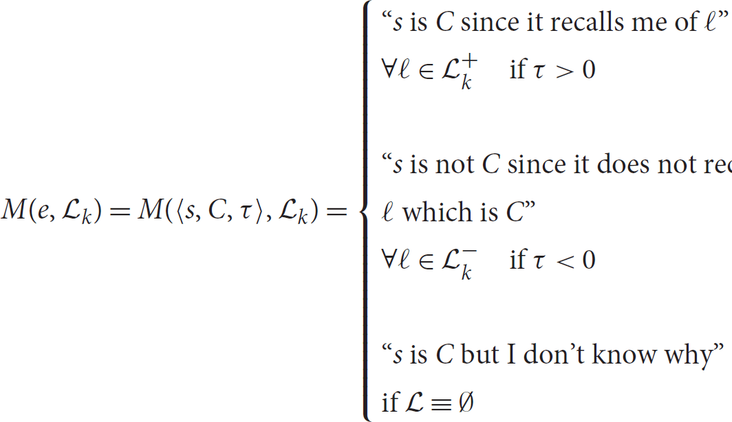$$ M(e,{\cal L}_k ) = M(\langle s,C,\tau \rangle ,{\cal L}_k ) = \left\{ {\matrix{ {{\rm{''{\it{s}}\,is\,C\,since\,it\,recalls\,me\,of\,\ell}}'' } \hfill \cr {{\kern 1pt} \forall \ell \in {\cal L}_k^ + \quad \;{\it{if}}\;\tau \; > \;0{\kern 1pt} } \hfill \cr \quad \hfill \cr {{\rm{''{\it{s}}\,is\,not\,{\it{C}}\,since\,it\,does\,not\,recall\,me\,of}}} \hfill \cr {\ell {\,\rm{which\,is\,{\it{C}}''}}} \hfill \cr {{\kern 1pt} \forall \ell \in {\cal L}_k^ - \quad \;{\it{if}}\;\tau \; < \;0{\kern 1pt} } \hfill \cr \quad \hfill \cr {{\rm{''{\it{s}}\,is\,{\it{C}}\,\,but\,I\,don't\,know\,why''}}} \hfill \cr {{\kern 1pt} {\rm{if}}\,{\cal L} \equiv \emptyset {\kern 1pt} } \hfill \cr } } \right. $$

where $$ {\cal L}_k^ + $$ and $$ {\cal L}_k^ - $$ are the partition of landmarks with positive and negative relevance scores in $${\cal L}_k$$, respectively.

Here we defined three explanatory models we used during experimental evaluation:

(Basic Model) The first model is the simplest. It returns an analogy only with the (unique) consistent landmark with the highest positive score if τ = 1 and lowest negative when τ = −1. In case no active and consistent landmark can be found, the Basic model returns a phrase stating only the predicted class, with no explanation. For example, given the triple e ₁ = 〈‘Put this plate in the center of the table’, THEME_PLACING, 1〉, that is an explanation for the Argument Classification task, the model would produce the following sentence:

I think “this plate” is THEME of PLACING in “Robot PUT this plate in the center of the table” since it reminds me of “the soap” in “Can you PUT the soap in the washing machine?”.

(Multiplicative Model) In a second model, denoted as multiplicative, the system makes reference to up to $$ k_1 \le k $$ analogies with positively active and consistent landmarks. Given the above explanation e ₁, and k ₁ = 2, it would return:

I think “this plate” is THEME of PLACING in “Robot PUT this plate in the center of the table” since it reminds me of “the soap” in “Can you PUT “the soap” in the washing machine?” and it also reminds me of “my coat” in “HANG my coat in the closet in the bedroom”.

(Contrastive Model) The last proposed model is more complex since it returns both a positive analogy (whether τ = 1) and a negative (τ = −1) analogy by selecting, respectively, the most positively relevant and the most negatively relevant consistent landmark. For instance, it could return:

I think “this plate” is the THEME of PLACING in “Robot PUT this plate in the center of the table” since it reminds me of “the soap” which is in “Can you PUT the soap in the washing machine” and it is not the GOAL of PLACING since different from “on the counter” in “PUT the plate on the counter”.

All three models find their foundations, from an argumentation theory perspective, in the argument by analogy schema (Walton, Reed, and Macagno Reference Walton, Reed and Macagno2008): as such a kind of arguments gains strength proportionally to the linguistic plausibility of the analogy, a user exposed to it will implicitly gauge the evidences from the linguistic properties shared between the input sentence (or its parts) and the one used for comparison as well their importance with respect to the output decision, hence endowing a different amount of trust in the machine verdict accordingly.

4.4 Using information theory for validating explanations

In general, judging the semantic coherence of an explanation is a very difficult task. In this section, we propose an approach which aims at evaluating the quality of the explanations in terms of the amount of information that a user would gather given an explanation with respect to a scenario where such explanation is not made available. More formally, let P (C|s) and P (C|s, e) be, respectively, the prior probability of the user believing that the classification of s is correct and the probability of the user believing that the classification of s is correct given an explanation. Note that both indicate the level of confidence the user has in the classifier (i.e., the KDA) given the amount of available information, that is, with and without explanation. Three kinds of explanations are possible:

• • Useful explanations: these are explanations such that C is correct and P(C|s,e) > P(C|s) or is not correct and P(C|s,e) < P(C|s)

• • Useless explanations: they are explanations such that P(C|s,e) = P(C|s)

• • Misleading explanations: they are explanations such that C is correct P(C|s,e) < P(C|s) or C is not correct and P(C|s,e) > P(C|s)

The core idea is that semantically coherent and exhaustive explanations must indicate correct classifications, whereas incoherent or nonexistent explanations must hint toward wrong classifications. Given the above probabilities, we can measure the quality of an explanation by computing the Information Gain (Kononenko and Bratko Reference Kononenko and Bratko1991) achieved: the posterior probability is expected to grow w.r.t. to the prior one for correct decisions when a good explanation is available against the input sentence while decreasing for bad or confusing explanations. The intuition behind Information Gain is that it measures the amount of information (provided in number of bits) gained by the explanation about the decision of accepting the system decision about an incoming sentence s. A positive gain indicates that the probability amplifies toward the right decisions and declines with errors. We will let users to judge the quality of the explanation and assign them a posterior probability that increases along with better judgments. In this way, we have a measure of how convincing is the system about its decisions as well as how weak is the system to clarify erroneous cases. To compare the overall performance of the different explanatory models M, the Information Gain is measured against a collection of explanations generated by M and then normalized throughout the collection’s entropy E as follows:

(10) $$ I_r = {1 \over E}{1 \over {|{\cal T}_s |}}\sum\limits_{j = 1}^{|{\cal T}_s |} I(j) = {{I_a } \over E} $$

where $${\cal T}_s$$ is the explanations collection and I(j) is the Information Gain of explanation j.

5.1 Training the KDA for complex semantic inferences

We conducted an extensive experimental investigation in order to demonstrate that the proposed KDA is an effective solution for combining the expressiveness of kernel methods with the powerful learning capabilities of Deep Learning. Furthermore, we will show that the KDA is very efficient and that it can easily scale to large datasets. Finally, we investigated the impact of linguistic information on the performance reachable by a KDA by studying the benefits that different kernels (each characterized by a growing expressive power) can bring to the accuracy in semantic inference tasks. We adopted the same architecture, without major differences, for both tasks, that is, QC and AC, and the good performances obtained in these rather different tasks clearly confirm that the proposed framework is a general solution with an extremely large applicability.

General experimental settings: the Nyström projector has been implemented in the KeLP framework (Filice et al. Reference Filice, Castellucci, Martino, Moschitti, Croce and Basili2018). The neural network has been implemented in Tensorflow,^{Footnote b} with two hidden layers whose dimensionality corresponds to the number of involved Nyström landmarks. The ReLU is the nonlinear activation function in each layer. The dropout has been applied in each hidden layer and in the final classification layer. The values of the dropout parameter and the λ parameter of the L₂-regularization have been selected from a set of values via grid-search. The Adam optimizer with a learning rate of 0.001 has been applied to minimize the loss function, with a multi-epoch (500) training, each fed with batches of size 256. We adopted an early stop strategy, where the best model was selected according to the performance over the development set. Every performance measure is obtained against a specific sampling of the Nyström landmarks with fixed sizes. Results averaged against 5 such samplings are always hereafter reported. In the following experiments, the only difference in the KDA configuration is the adopted kernels that will be described specifically for each task.

5.1.1 Semantic inferences: Question classification

QC is the task of mapping a question into a closed set of answer types in a Question Answering system. The adopted UIUC dataset (Li and Roth Reference Li and Roth2006) includes a training and test set of 5, 452 and 500 questions, respectively, organized in six classes (like ENTITY or HUMAN). TKs resulted very effective, as shown in Croce, Moschitti, and Basili (Reference Croce, Moschitti and Basili2011) and Annesi, Croce, and Basili (Reference Annesi, Croce and Basili2014).

A first experiment aims at understanding the impact of different kernels into the proposed KDA framework. The input vectors for the KDA are modeled using the Nyström method (with different kernels) based on a number of landmarks ranging from 100 to 1000. We tried different kernels with increasing expressiveness:

• • BOWK: a liner kernel applied over bag-of-words vectors having lemmas as dimensions. It provides a pure lexical similarity.

• • PTK: the partial tree kernel over the GRCT representations. It provides a lexical and syntactic similarity.

• • SPTK: the smoothed partial tree kernel over the GRCT representations. It improves the reasoning of the PTK by including the semantic information derived by word embeddings.

• • CSPTK: the compositionally smoothed partial tree kernel over the GRCT representations. It adds the semantic compositionality to the SPTK.

In the SPTK and CSPTK, we used 250-dimensional word vectors generated by applying the Word2vec tool with a Skip-gram model (Mikolov et al. Reference Mikolov, Chen, Corrado and Dean2013) to the entire Wikipedia. The TKs have default parameters (i.e., μ = λ = 0.4).

Figure 6: QC task—accuracy measure curves w.r.t. the number of landmarks.

Figure 6 shows the impact of different kernels in the proposed KDA model, whereas the different plots are based to a varying number of landmarks in the Nyström formulation. The increasing complexity of the investigated kernels directly reflects on the accuracy achieved by the KDA. The BOWK is the simplest kernel and obtains poor results: it needs 800 landmarks to reach 85% of accuracy.

The contribution of the syntactic information provided by TKs is straightforward. The PTK achieves about 90% of accuracy starting from 600 landmarks. These results are significantly improved by SPTK and CSPTK when the semantic information of the word embeddings is employed: even when only 100 landmarks are used, the KDA using these kernels can obtain 90% of accuracy and overcomes 94% with more landmarks. These achievements demonstrate that the KDA results directly depend on the involved kernel functions and that the improvement guaranteed by using a more expressive kernel cannot be obtained by the nonlinear learning of the Neural Network.

We also performed a second set of experiments to show that (i) the proposed KDA is far more efficient than a pure kernel-based approach, and (ii) the powerful nonlinear learning provided by the neural networks is necessary to take the best from the Nyström embeddings and achieve higher accuracies. In this case, we focused on the most accurate kernel, that is, the CSPTK. The kernel-based SVM formulation by Chang and Lin (Reference Chang and Lin2011), fed with the CSPTK (hereafter SVM_ker), is here adopted to determine the reachable upper bound in classification quality, that is, a 95% of accuracy, at higher computational costs. It establishes the state-of-the-art over the UIUC dataset. The resulting model includes 3,873 support vectors: this corresponds to the number of kernel operations required to classify any input test question.

To justify the need of the Neural Network, we compared the proposed KDA to an efficient linear SVM that is directly trained over the Nyström embeddings. This SVM implements the Dual Coordinate Descent method (Hsieh et al. Reference Hsieh, Chang, Lin, Keerthi and Sundararajan2008) and will be referred as SVM_lin.

Results are reported in Table 1: computational saving refers to the percentage of avoided kernel computations with respect to the application of the SVM_ker to classify each test instance. We also measured the performance of the Convolutional Neural Network^{Footnote c} (CNN) of Kim (Reference Kim2014) that achieves the remarkable accuracy of 93.6%. Zhou et al. (Reference Zhou, Sun, Liu and Lau2015) report results from a different version of LSTM, including a Bidirectional LSTM (BiLSTM) and the combination of a Convolutional and a Recurrent Neural Network (namely C-LSTM) that leads to an Accuracy of 94.6%.

Table 1: Results in terms of accuracy and saving in the QC task. In brackets, accuracy scores of the linear classifier SVM_lin

Notes: Accuracy scores of the linear classifier SVM_lin are given in brackets.

Note that the linear classifier SVM_lin operating over the approximated kernel space achieves the same classification quality of the CNN when only 1000 landmarks are considered. KDA improves these results, achieving 94.3% accuracy even with fewer landmarks (only 600), showing the effectiveness of nonlinear learning over the Nyström input. Although SVM_ker improves to 95%, KDA provides a saving of more than 84% kernel computations at classification time. This result is straightforward as it confirms that (1) linguistic information encoded in a tree is important in the analysis of questions, (2) Nyström vectors correspond to very expressive sentence embeddings, and (3) they can be used effectively in the pretraining stage of an MLP. Moreover, even if the application of the KDA does not outperform the results obtained by the C-LSTM (even if the results are very close), it is worth noting that the proposed classifier is a very simple multilayered feed-forward network applied in a very informative space. Further extensions which use more complex architectures in such spaces represent an important research direction. Figure 7 shows the accuracy curves according to various approximations of the kernel space, that is, number of landmarks.

5.1.2 Semantic inferences: Argument Classification in Semantic Role Labeling

Semantic role labeling (SRL; Palmer, Gildea, and Xue Reference Palmer, Gildea and Xue2010) consists in detecting the semantic arguments associated with the predicate of a sentence and their classification into their specific roles (Fillmore Reference Fillmore1985). For example, given the sentence “Bring the fruit onto the dining table”, the task would be to recognize the verb “bring” as evoking the BRINGING frame, with its roles, THEME for “the fruit,” and GOAL for “onto the dining table”. AC corresponds to the subtask of assigning labels to the sentence fragments spanning individual roles.

Figure 7: QC task—accuracy curves w.r.t. the number of landmarks.

As proposed in Moschitti, Pighin, and Basili (Reference Moschitti, Pighin and Basili2008), SRL can be modeled as a multi-classification task over each parse tree node n, where argument spans reflect sub-sentences covered by the tree rooted at n. Consistently with Croce, Moschitti, and Basili (Reference Croce, Moschitti and Basili2011), in our experiments the KDA has been empowered with an SPTK, operating over GRCT derived from dependency grammar, as shown in Figure 9.

Figure 8: A dependency graph associated with “ Carry the book to my nightstand”.

Figure 9: GRCT of the command “Carry the book to my nightstand”.

We used the HuRIC dataset (Bastianelli et al. Reference Bastianelli, Castellucci, Croce, Iocchi, Basili and Nardi2014; Bastianelli et al. Reference Bastianelli, Croce, Vanzo, Basili and Nardi2016), including over 650 annotated transcriptions of spoken robotic commands, organized in 18 frames and about 60 arguments. We extracted single arguments from each HuRIC example, for a total of 1300 instances. We run experiments with a methodology similar to the one described in Section 5.3, but due to the limited data size we performed extensive 10-fold cross-validation, optimizing network hyper-parameters via grid-search for each test set. We generated Nyström representation of a equally weighted linear combination of SPTK function with default parameters and μ = λ = 0.4 of linear kernel function applied to sparse vector representing the instance frame. With these settings, the KDA accuracy was 96.1%.

5.2 Experimental evaluation of explanatory models

The effectiveness of the proposed approach has been measured against two different semantic processing tasks, that is, QC and AC in semantic role labeling. The KDA evaluated in Section 5.1 is here adopted and extended with LRP. For evaluating our explanation method, we defined five quality categories and associated them with values for the posteriori probability P(C|s,e), as shown in Table 2. We gathered into explanation datasets hundreds of explanations from the three models for each task and presented them to a pool of annotators (further details in related subsections) for independent labeling. During the annotation process, annotators are exposed to examples classified by the KDA with an explanation and they are asked to label the explanation with one of the following classes: Very Good if the provided explanation is clearly convincing, Good if the explanation is convincing but it is not completely related to the input example so that some doubts about the system decision still remain, Weak if the explanation is not useful to increase the confidence of the user with respect to the system decision, Bad if the explanation makes the annotator believe that the system decision is not correct, while Incoherent corresponds to the case where the explanation is clearly inconsistent with the input example and suggests a clear error of the system in providing its answer. Annotators had no information of the correctness of the system emissions but just knowledge about the dataset entropy. We addressed their consensus by measuring a weighted Cohen’s Kappa (adopting the weights reported in Table 3).

Table 2. Posterior probabilities w.r.t. quality categories

Table 3. Weights for the Cohen’s kappa k _w statistics

5.3 Evaluating question classification

We generated the Nyström representation of the CSPTK (Annesi, Croce, and Basili Reference Annesi, Croce and Basili2014) function with default parameters μ = λ = 0.4. Using 500 landmarks, the KDA accuracy was 92.6%.

Table 4. Information gains for the three explanatory models applied to the SRL-AC and QC datasets. k _w is the weighted Cohen’s kappa k _w

A group of three annotators evaluated an explanation dataset of 300 explanations (perfectly balanced between correct and not correct classification), composed of 100 explanations for each model. Performances are shown in Table 4: all three explanatory models were able to gain more than half the required information in order to ascertain the correctness of the classification. As an example, consider:

The model provided an evidently coherent analogy, but this is a easy case due to the occurrence in both questions of very discriminative words, i.e “what year.” However, the system is also able to capture semantic similarities when both syntactic and lexical features are different. For example:

This is an high-quality explanation since the system provided an analogy with a landmark requesting the same fine-grained category but with little sharing of lexical and syntactic information (note, for example, the absence in the landmark of the very discriminative word “where”). Let us now consider the case of wrong classification:

The system provided an explanation that is not possible to easily interpret: indeed, it was labeled as [Incoherent] by all the annotators.

However, the system suffers for two issues. First, in the case of negative modality and correct classification, explanations, albeit coherent, can be trivial and do not actually help in reducing uncertainty about the correct target class. For example,

Here the explanation is correct but obvious; instead, a negative analogy with a very likely class, that is, ENTITY or DESCRIPTION, would have provided some disambiguation. Moreover, some questions are inherently ambiguous due to the lack of a broader context. This can lead to prediction errors and as well as to user actually being misled by the explanation, for example,

In this example, the explanation makes NUMBER to appear as a more likely target for the question than ENTITY, although seemingly correct this is not the right label. Here the lack of contextual information in the question itself is the case.