TESTING FOR UTILITY MAXIMIZATION: GARP

This section focuses on GARP as defined by Varian (1982) within the Samuelson's (1947) revealed preference theory. Let x_i=(x_i1, x_i2, …, x_ik)′, i∈{1, …, T} be a (k×1) vector of observed real quantities, and let p_i=(p_i1, p_i2, …, p_ik)′, i∈{1, …, T} be the associated prices. Let the set D={(x_i, p_i)∈(R⁺)^2k, i=1, …, T} thus grouping a finite number of observations of the couples (x_i, p_i). Varian (1982), extending Afriat's (1967, 1973) work, has suggested an operational procedure to test if a dataset D behaves as if it were generated by utility maximization.

First, define the binary strict direct revealed preference relation P⁰ by x_iP⁰x_j if p_i·x_i>p_i·x_j i∈{1, …, T}, j∈{1, …, T}, and the (T×T) P⁰ matrix, whose element p⁰_ij (ith row, jth column) is defined as follows:

Similarly, define the binary direct revealed preference relation R⁰ by x_iR⁰x_j if p_i·x_i[ges ]p_i·x_ji∈{1, …, T}, j∈{1, …, T}, and the (T×T) R⁰ matrix, whose element r⁰_ij is defined as follows:

At last, define the binary revealed preference relation R by x_iRx_j if there exists a sequence between x_i and x_j such that p_i·x_i[ges ]p_i·x_m, p_m·x_m[ges ]p_m·x_n, …, p_p·x_p[ges ]p_p·x_j, or x_iR⁰x_m, x_mR⁰x_n, …, x_pR⁰x_j, where R is the transitive closure of R⁰. Define the (T×T) R matrix, whose element r_ij is defined according to the Warshall's algorithm (see Appendix A).

Using the above definitions, GARP is defined as follows:

DEFINITION 1 [Varian (1982)]. The data satisfy the general axiom of revealed preference if ∀i∈{1, …, T}∀j∈{1, …, T} x_iRx_j implies not x_jP⁰x_i (r_ij=1 does not imply p⁰_ji=1) or x_iRx_j[xrArr ]p_j·x_j[les ]p_j·x_i.

If x_i is revealed preferred to x_j, then x_j cannot be strictly directly revealed preferred to x_i. Using GARP, Varian (1982) proved the following theorem.

THEOREM 1 [Varian (1982)]. For a set D, the three following conditions are equivalent:

1. There exists a locally nonsatiated utility function U(·) that rationalizes the data.
2. There exist strictly positive utility indices U_i and marginal income indices λ_i that satisfy ∀i∈{1, …, T}∀j∈{1, …, T} the Afriat inequalities (1),
   
3. The data satisfy GARP.

Hence, since GARP is both necessary and sufficient for utility maximization, the decision rule is

Varian's decision rule is rather stringent since a single violation of the axiom leads to rejection of the maximization hypothesis. Nevertheless, violations of the axiom may be caused by purely stochastic elements as measurement error, data being actually consistent with the maximization principle. Hence, when implementing GARP, it is crucial that one should distinguish significant from nonsignificant violations, that is, between violations caused by stochastic elements and violations caused by some ruptures in the utility function or by a nonmaximization behavior. We next introduce such a procedure.

TESTING THE VIOLATIONS OF GARP FOR THEIR SIGNIFICANCE

In Varian's (1982) work, two strong assumptions are made: (i) data are measured without error and (ii) agents are perfectly rational, adjusting quantities at once following a movement in prices. In this paper, we deal only with the first point.³

Assumption 1. Under the null hypothesis, data D={(x*_i, p_i)∈(R⁺)^2k, i=1, …, T} behave as if they were generated by an optimization behavior.

Assumption 2. Under the null hypothesis, prices are perfectly known and measured, but quantities x*_i are unobservable. In particular, we consider the stochastic generating mechanism⁴

where ε_ij is distributed as f(θ); f(θ) possesses finite absolute moments up to fourth order, in particular, with E(ε_ij)=0 and V(ε_ij)=σ².

In (2), ε_ij can be seen either as a measurement error or as an optimization error. In this case, x*_i appears to be a theoretical demand, whereas x_i is the realized one. In the following, we use the term measurement error to speak about those two concepts.

Empirically, the magnitude of the measurement error as well as f(θ) are generally unknown. Thus, following Varian (1985), and given the multiplicative relationship (2), we compute the minimal perturbation in the data in order to satisfy GARP. This is achieved by solving over z_ij the quadratic program (3):

subject to ∀i∈{1, …, T}∀j∈{1, …, T}z_iRz_j implies not z_jP⁰z_i.

Let

be the solution of the above program, and define the realization

as

.

Assumption 3. Given Assumptions 1 and 2, under the null,

is distributed as g(β), where g(·) is not necessarily equal to f(·) and g(β) possesses finite absolute moments up to fourth order, in particular with

and

.

Note that Assumption 3 emphasizes a clear distinction between the true and unobservable measurement error

and

, which is the minimal adjustment, in order to satisfy GARP. Since some measurement errors will cause violations, and other will not, especially for bundles that are far in constant terms, there is no reason why

and ε_ij will match and then have the same distribution. Thus, in this work, the main assumption is that, under the null, the computed adjustment inherit the i.i.d. property of the true errors.⁵

With the above comments in mind, at least three strategies can be used to test the necessary adjustment for its significance. The first one consists of assuming a particular form for g(β), and then testing if

follows g(β). Second, by using the central limit theorem as in Yatchew and Epstein (1985), one can derive a statistic asymptotically distributed as N(0, 1). Nevertheless, this strategy requires the knowledge of the first and second moments of the true errors, which is generally unknown in empirical work. At last, since Assumption 3 implies that the adjustment is i.i.d., testing the adjustment for its significance can be achieved simply by implementing i.i.d. tests. This is the strategy used in this paper.

To implement i.i.d. tests, two sets of residuals can be used: s¹ and s² (s² being a subset of s¹). They are defined as follows. Let

be a (T×k) matrix whose element at the ith row and jth column is given by

and let s¹ be a (Tk×1) vector defined as

The first T elements of s¹ form a sample realization of the errors associated with good 1, the T + 1 to 2T elements are the T realizations of the errors associated with good 2, and so on. As our procedure leads to focus on only a few bundles, an alternative set of residuals can also be used. Let

be a (r×k) matrix whose element at the ith row and jth column is given by

if and only if

, r being the number of bundles altered to ensure the compatibility with GARP. Let

. The first r elements of s² are the r realizations of the errors associated with good 1, the r + 1 to 2r elements are the r realizations of the errors associated with good 2, and so on.

Given s¹ or s², following Spanos (1999), testing if residuals are i.i.d. is achieved by estimating two auxiliary regressions and by testing restrictions. For first-order dependence and trend heterogeneity, we estimate (4) and test the joint significance of the coefficients α and γ_j, j=1, …, τ1 by using an F-test, or a Wald test. For second-order dependence and trend heterogeneity, we estimate (4) and test the joint significance of the coefficients δ and β_jk, j, k=1, …, τ2 by using an F-test, or a Wald test.⁶

where

Let P₁ and P₂ be the probabilities associated with the Fisher or the Wald test, respectively, for (4) and (4). The decision rule at a threshold α is then

We next explain how the quadratic program is solved.

SOLVING THE PROCEDURE

In this section we explain how the quadratic program (3) is solved. Basically, if GARP is satisfied for a dataset D, then, by definition, there exist ∀i∈{1, …, T}∀j∈{1, …, T} indices satisfying the Afriat inequalities (Theorem 1). It is thus possible to order all the bundles (or observations) into a coherent sequence according to either utility indices U_i satisfying (1) (cardinal) or by simply using the transitive closure matrix R (ordinal). Indeed, this latter contains all the transitive relations. We call this unique transitive sequence, in which all bundles are linked by the binary relation [sccue ] (standing for “preferred or indifferent to”), a preference chain. We say that a bundle x_i is located at the nth place in the preference chain if it is revealed as preferred to T−n bundle(s) (excluding x_i). For example, if n=1, then x_i is at the top of the preference chain, being revealed as preferred to all the other bundles, implying U(x_i)[ges ]U(x_j), ∀j∈{1, …, T}; if n=T, then x_i is at the bottom of the preference chain, all the other bundles being revealed as preferred to it, implying U(x_i)[les ]U(x_j), ∀j∈{1, …, T}. If GARP is violated, it is not possible to order all the bundles. Hence, solving (3) amounts to rebuilding a preference chain, such that for this sequence the objective function is minimal.

We now explain how the violations of GARP affect the transitive closure matrix and thus the preference chain. We first introduce some definitions.

DEFINITION 2. Two observations x_i and x_j satisfy the binary relation x_iVRx_j if x_iRx_j and x_jP⁰x_i (i.e., if r_ij=1 and p⁰_ji=1), or if there exists a sequence between x_i and x_j such that x_iRx_k and x_kP⁰x_i, x_kRx_l and x_lP⁰x_k, …, x_mRx_j and x_jP⁰x_m. We call such a sequence a violation chain.

DEFINITION 3. Two observations x_i and x_j satisfy the binary relation x_iSRx_j if S(i)=S(j), where S(i)=([sum ]^T_j=1r_ij)−1 is a function returning the sum m of the elements of the ith row of the transitive closure matrix, minus 1. With 0[les ]m[les ]T−1 indicating to how many bundles x_i is revealed preferred to (excluding itself).

PROPOSITION 1. For two observations x_i and x_j, satisfying x_iVRx_j implies x_iSRx_j.

Proposition 1 follows directly from the Warshall's algorithm. If x_i is directly revealed preferred to x_k, x_k is directly revealed preferred to x_l, …, and this latter is directly revealed as preferred to x_j, then we will have, by using the Warshall's algorithm x_iRx_k, x_iRx_l, …, x_iRx_j and S(i)=m. If x_iVRx_j, we have r_ij=1 and p⁰_ji=1; that is, p_j·x_j > p_j·x_i, implying x_jRx_i. Hence, by the Warshall's algorithm, x_j is going to be revealed preferred to x_i, and to all the bundles x_i was revealed preferred to implying S(j)=m and thus x_iSRx_j.⁷

Let V∈D, be a set grouping all the unique observations (x_i, p_i), violating one or several times GARP. For example, if we have the violations x₁Rx₃ and x₃P⁰x₁, x₂Rx₁ and x₁P⁰x₂, x₂Rx₃ and x₃P⁰x₂, and x₃Rx₂ and x₂P⁰x₃, then V={(x₁, p₁), (x₂, p₂), (x₃, p₃)}.

PROPOSITION 2. There exist(s) B_l set(s), l=1, …, n such that B₁∪B₂∪…∪B_n=V, B₁∩B₂∩…∩B_n=[empty ] and such that every couple (x_i, p_i)∈B_l, (x_j, p_j)∈B_l ∀l∈{1, …, n} satisfy x_iSRx_j.

Proposition 2 follows directly from Proposition 1. It states that the bundles violating GARP can be ordered in n, set(s) B_l, l=1, …, n, and that each set contains bundles that are potential candidates to be at the same position in the preference chain. In each set, all the bundles enter at least one violation chain. Let N_l, be the number of bundles (or observations) in a set B_l. From Proposition 2, it follows that we thus have a priori at least n ruptures in the preference chain, and thus [prod ]ⁿ_l=1N_l! possible preference chains.

To illustrate this, let the set D₁={(x_i, p_i)∈(R⁺)^2k, i=1, …, 5}, thus grouping five observations of the couple (x_i, p_i), and let the matrices P⁰₁, R⁰₁ and R₁, represent the preferences.

Four violations appear, giving the set V={(x₂, p₂), (x₃, p₃), (x₄, p₄), (x₅, p₅)}. As x₂VRx₃ (and x₃VRx₂), x₄VRx₅ (and x₅VRx₄), S(2)=3, S(3)=3, S(4)=1, S(5)=1, the set V can be broken up into two subsets B₁ and B₂ such that B₁∪B₂=V and B₁∩B₂=[empty ], where B₁={(x₂, p₂), (x₃, p₃)} and B₂={(x₄, p₄), (x₅, p₅)}. The set B₁ contains bundles that are all candidates to be located at the second place in the preference chain, and the set B₂ contains bundles that are potentially at the fourth place in the chain, giving a priori [prod ]²_l=1N_l!=2!*2!=4 possible preference chains. These latter are given by (6):

It is thus apparent that solving the quadratic program (3) amounts to finding, in each set B_l, the bundle that will be revealed preferred to the other bundle(s) of the set, that is, to rebuild a coherent preference chain. We next explain how, in each set, the unobserved bundles

are computed, and then we introduce an iterative procedure.

Computing the Bundles

Suppose that for a dataset D, GARP is violated, and let B₁ be one of the n set(s). For reasons that will become apparent later, define B₁ such that for (x_i, p_i)∈B₁ and (x_j, p_j) ∉ B₁, S(i)>S(j). Let for a couple {(x_i, p_i), (x_j, p_j)} (x_i, p_i)∈B₁, (x_j, p_j)∈B₁ such that x_iRx_j and x_jP⁰x_i, the quadratic program (7), minimized over z_ij:

Empirically, the constraint of (7) is replaced by only two kinds of constraints, which are defined as follows:

The two kinds of constraints above ensure that (i) ∀x_j, z_iVRx_j will not hold any more, (ii) z_i will not cause new violations with bundles it was revealed preferred to (directly or indirectly), (iii) z_i will be located at a given place in the preference chain.⁹

Given (7), to rebuild a preference chain, that is, to choose the bundle z_i which will be revealed preferred to the other bundles of the set B₁, we solve (7) for each (x_i, p_i)∈B₁ violating GARP, and choose the one having the minimal objective function obj_i. This bundle,

, will be revealed preferred to the others of the set.

An Iterative Procedure

The above procedure, consisting of solving (7) for each bundle of a set B₁, and then choosing the one having the minimal objective function, can be implemented to rebuild a preference chain, independently for all sets if and only if N_l=2 ∀l∈{1, …, n}. The reason is that if ∃l∈{1, …, n} such that N_l > 2, then nothing ensures that finding the bundle

and replacing (x_i, p_i) by

in D, the other bundles of the set B_l will not violate GARP, being now candidates to be at a lower place in the preference chain. To deal with this problem, we propose the following four-step iterative procedure:

Step 1. Test D for consistency with GARP, let nvio be the number of violations [0[les ]nvio[les ]T(T−1)]

Step 2. Build a set V and n set(s) B_l, l=1, …, n. Go to step 3.

Step 3. Among the sets B_l, search for the one written B₁, containing the bundles being potentially at the same highest place in the preference chain, such that if n>2 for (x_i, p_i)∈B₁ and (x_j, p_j) ∉ B₁: S(i)>S(j). Go to step 4.

Step 4. In the set B₁, search, by using (7), for the bundle that will be revealed as preferred to the others, such that, for this bundle, among all objective functions, its objective function is minimal. Let

be the bundle solution of this procedure. Replace, in D, (x_i, p_i) with

and go to step 1.

We now illustrate this procedure.

IMPLEMENTATIONS

In this section, we illustrate the iterative procedure by two examples. Let the dataset D₁={(x_i, p_i)∈(R⁺)^2k, i=1, …, 5}, for which the preferences are given by the above P⁰₁, R⁰₁ and R₁ matrices. As we have seen, four violations give the sets V={(x₂, p₂), (x₃, p₃), (x₄, p₄), (x₅, p₅)}, B₁={(x₂, p₂), (x₃, p₃)}, and B₂={(x₄, p₄), (x₅, p₅)}. As S(2)=3, S(3)=3, S(4)=1, S(5)=1, the procedure consists in first finding which of the two bundles in B₁ will be at the second place in the preference chain. This is achieved by solving (7) over z₂ subject to p₂·z₂=p₂·x₂, p₃·x₃[les ]p₃·z₂, and p₄·x₄[les ]p₄·z₂, p₅·x₅[les ]p₅·z₂(since r₂₄=1 and r₂₅=1), and then (7) over z₃ subject to p₃·z₃=p₃·x₃, p₂·x₂[les ]p₂·z₃, and p₄·x₄[les ]p₄·z₃, p₅·x₅[les ]p₅·z₃. Then, choose the bundle z_i, i∈{2, 3} for which the objective function obj_i is minimal. Assuming, for example, that obj₂<obj₃, replace x₂ with the computed value

in D₁. Rerunning GARP gives now the following preferences:

Only two violations appear giving the set V=B₁={(x₄, p₄), (x₅, p₅)}, and a priori 2! two possible preference chains:

Similarly, solve (7) over z₄ and z₅, subject to, respectively, p₄·z₄=p₄·x₄, p₅·x₅[les ]p₅·z₄ for the first program and p₅·z₅=p₅·x₅, p₄·x₄[les ]p₄·z₅ for the second program. Then, choose z_i, i∈{4, 5} such that the corresponding obj_i is minimal. Suppose that obj₄>obj₅; then, the final preferences are given by the following P⁰₁, R⁰₁, and R matrices, and the coherent preference chain by (9):

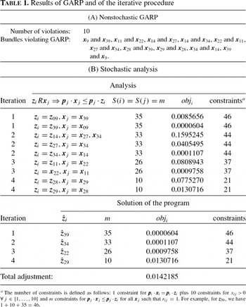
Consider now a numerical application. Let D₂={(x_i, p_i)∈(R⁺)²⁰, i=1, …, 40} be a set of simulated data, where quantities x*_ij, i=1, …, 40, j=1, …, 10, are solution of a Cobb-Douglas maximization program (see next section), and x_ij is related to x*_ij by the relationship (2), where ε_ij is distributed as N(0, 0.2²) (see Tables (B.1) and (C.1) in Appendixes B and C). Table 1 presents both the results of GARP and of the iterative procedure.

Running GARP, 10 violations appear, giving the set V={(x₉, p₉), (x₁₁, p₁₁), (x₁₄, p₁₄), (x₂₂, p₂₂), (x₂₇, p₂₇), (x₂₈, p₂₈), (x₂₉, p₂₉), (x₃₄, p₃₄), (x₃₉, p₃₉)} and 4 sets: B₁={(x₉, p₉), (x₃₉, p₃₉)}, B₂={(x₁₄, p₁₄), (x₂₇, p₂₇), (x₃₄, p₃₄)}, B₃={(x₁₁, p₁₁), (x₂₂, p₂₂)}, and B₄={(x₂₈, p₂₈), (x₂₉, p₂₉)}. As there are more than two bundles in the set B₂, we run the iterative procedure. The set B₁ contains two bundles that are revealed preferred to all the others in the other sets. Thus, we first search (iteration 1 of the procedure) if z₉Rx₃₉[xrArr ]p₃₉·x₃₉[les ]p₃₉·z₉ or if z₃₉Rx₉[xrArr ]p₉·x₉[les ]p₉·z₃₉. The two objective functions associated with these two hypotheses are, respectively, 0.0085656 and 0.0000604. Since 0.0000604<0.0085656, we conclude that z₃₉Rx₉[xrArr ]p₉·x₉[les ]p₉·z₃₉, that is, z₃₉ will be at the fifth place in the preference chain. Replacing in D₂ x₃₉ with

and rerunning GARP (iteration 2) now gives eight violations and the sets V={(x₁₁, p₁₁), (x₁₄, p₁₄), (x₂₂, p₂₂), (x₂₇, p₂₇), (x₂₈, p₂₈), (x₂₉, p₂₉), (x₃₄, p₃₄)}, B₁={(x₁₄, p₁₄), (x₂₇, p₂₇), (x₃₄, p₃₄)}, B₂={(x₁₁, p₁₁), (x₂₂, p₂₂)}, and B₃={(x₂₈, p₂₈), (x₂₉, p₂₉)}.

Focusing on the set B₁, as previously, as for (x_i, p_i)∈B₁ and (x_j, p_j) ∉ B₁S(i) > S(j), three hypotheses are tested: z₁₄Rx₂₇[xrArr ]p₂₇·x₂₇[les ]p₂₇·z₁₄, z₁₄Rx₃₄[xrArr ]p₃₄·x₃₄[les ]p₃₄·z₁₄, z₂₇Rx₃₄[xrArr ]p₃₄·x₃₄[les ]p₃₄·z₂₇, and z₃₄Rx₁₄[xrArr ]p₁₄·x₁₄[les ]p₁₄·z₃₄. Since we have min (0.1565245, 0.0405495, 0.0001107)=0.0001107, we conclude that z₃₄Rx₁₄[xrArr ]p₁₄·x₁₄[les ]p₁₄·z₃₄ and of course that z₃₄Rx₂₇[xrArr ]p₂₇·x₂₇[les ]p₂₇·z₃₄, z₃₄ being located at the seventh place in the preference chain. Replacing x₃₄ by

in D₂ and rerunning GARP (iteration 3), now gives four violations¹⁰

and rerun GARP (iteration 4). Only two violations appear giving the set V=B₁={(x₂₈, p₂₈), (x₂₉, p₂₉)}. Since the adjustments associated with z₂₈Rx₂₉[xrArr ]p₂₉·x₂₉[les ]p₂₉·z₂₈ and z₂₉Rx₂₈[xrArr ]p₂₈·x₂₈[les ]p₂₈·z₂₉ are, respectively, 0.077527 and 0.0130716, we choose z₂₉ as the solution of the iteration 4. Replacing x₂₉ with

in D₂, and rerunning GARP gives no more violation.¹¹

Thus, 10 violations for 40 observations and 10 goods in each bundle are ruled out only by altering 4 bundles, with a total adjustment of 0.0142185. Now, let's turn to some statistical inference. Figure 1 plots the vector s², where

,

are the first four observations,

,

,

,

, are the observations 4 to 8

,

,

,

are the observations 36 to 40. Tables 2 and 3 present the results of the i.i.d. tests (first and second order) for s¹ and s². In addition, to test for independence, two statistics are also computed: the Ljung-Box Q-stat and the McLeod-Li ML-stat. Both tables are structured as follows: The first part is related to independence tests, whereas the second part is dedicated to i.i.d. tests. Concerning the latter, we first select the order τ₁ and τ₂ for the auxiliary regressions (4) and (4) by using F-tests (Wald tests are also presented). Second, given the selected models, we present the i.i.d. tests. Here, for the set s¹, we choose τ₁=1 and τ₂=1. For those models, the probabilities associated with the i.i.d. tests, respectively, for the first and second order are 0.2088 (Wald 0.2075) and 0.3876 (Wald 0.3867) leading us to accept the i.i.d. hypothesis. Similar conclusions are drown from Table 3, the probabilities being, respectively, 0.1321 (Wald 0.1174) and 0.3434 (Wald 0.3324) for τ₁=1 and τ₂=1. Thus, in both cases, we accept

. Violations are caused by measurement error, which is coherent with our data generating process.

s2, i.i.d. data.

MONTE CARLO SIMULATIONS

In this section, we run Monte Carlo simulations to (i) estimate the power of GARP under measurement error; (ii) estimate the type I and II errors of the procedure; (iii) present, under the null, some key results about the distribution of the law of residuals, since g(·) and f(·) are unlikely to match. We first introduce our data generating process.

To estimate the type I error, that is, the probability of rejecting maximization, whereas there is maximization, we proceed as follows:

Step 1. We generate 10 series of prices, each series having 40 observations. Each series is defined as a random walk. For instance, for a period i∈{1, …, 40} and for a good j∈{1, …, 10}, p_ij is defined as

where ν_ij is a normally distributed term with zero mean and unit variance.

Step 2. In a similar way, we generate a series of income {\bf I}. For a period i∈{1, …, 40}, the income I_i is defined as

where ε_i is a normally distributed term with zero mean and unit variance.

Step 3. Given the above prices and income, we solve a maximization program for a Cobb-Douglas function. For a period i∈{1, …, 40}, the vector x*_i=(x*_i1, x*_i2, …, x*_i10)′ is the solution of (10), where

.

where

Step 4. We compute x_i=(x_i1, x_i2, …, x_i10)′ related to x*_i by the relationship

where ε_ij is a normally distributed term with zero mean and standard error σ.

Step 5. We build the set D={(x_i, p_i)∈(R⁺)²⁰, i=1, …, 40} and run the procedure; that is, we find the minimal adjustment, compute τ₁ and τ₂ by using F-tests or Wald tests, and test for i.i.d.-ness.

We repeat steps 1 to 5, 10,000 times for three different measurement errors: σ=5%, σ=10%, and σ=15%. We compute the type I error of GARP and of the procedure (at a threshold α) defined respectively as (12) and (13).

To estimate the type II error, we first need a definition of a “random behavior.” We will say that a dataset D is rationalized by a unique utility function if its parameters are constant over the entire period. We will say that there is a random behavior if the parameters a_ij change every periods. Thus, in our definition of the random behavior, a utility function rationalizes the data each period, but the weights change from one period to another.¹²

Step 3. Given prices and income, we solve a maximization program, where preferences are given by a Cobb-Douglas function. For a period i∈{1, …, 40}, the vector x*_i=x_i=(x_i1, x_i2, …, x_i10)′ is the solution of gram (14), where for j=1, …, 10, ∀(i, t)∈{1, …, 40} and i ≠ t:a_ij ≠ a_tj; a_ij=b_ij/[sum ]¹⁰_j=1b_ij, and b_ij∈[0, 1] is a uniformly distributed term.

where

and i ≠ t:a_ij ≠ a_tj,

where

is a uniformly distributed term.

Step 4. We build the set D={(x_i, p_i)∈(R⁺)²⁰, i=1, …, 40}, and run the procedure; that is, we find the minimal adjustment, we compute τ₁ and τ₂ by using F-tests or Wald tests, and test for i.i.d.-ness.

We repeat steps 1 to 410,000 times and compute the type II error of GARP and of the procedure (at a threshold α), respectively, defined by (15) and (16):

Tables 4 and 5 give the results of the simulations for three different standard errors and at four different thresholds. Table 4 focuses on the power of GARP and presents some summary statistics about the iterative procedure. Concerning GARP, it appears that, on the one hand, the test is extremely powerful against the random behavior hypothesis, since the type II error is null. On the other hand, when data are rationalized by a utility function, but are measured with errors, GARP seems accurate only for a very small measurement error¹³

Table 5 presents the type I and II errors associated with the i.i.d. tests for s¹ and s². At the usual threshold of 5%, the procedure appears to be quite powerful. Indeed, the type I error does not exceed 8.91% for a large measurement error for s² (10.39% for s¹) and is less than 5% for a small measurement error for s¹ and s². Concerning the type II error, it is about 5% for s² (8.54% for s¹), indicating that the probability of accepting maximization whereas there is not maximization is small. By way of comparison with Figure 1, we plot the necessary adjustment when data are generated at random (non-i.i.d. set), Figure 2. One will also note that s¹ and s² return approximately the same information. Nevertheless, using s² in empirical work seems more accurate giving the type II error and the type I error for a large measurement error.

s2, non-i.i.d. data.

At last, since Assumption 3 appears to be empirically justified, the question arises about the distribution of the residuals. Basically, the minimization program (3) may appear as some kind of regression under linear constraints. Then, the question arises about whether the residuals are normally distributed. To investigate the distribution of the adjustment, we have collected, at each of the 10,000 iterations concerning the estimation of the type I error, the sets s². We thus have three sets corresponding to the three measurement errors: σ=0.05, 0.10, and 0.15. Table 6 presents some summary statistics about the three distributions as well as two normality tests. In the Cobb-Douglas framework, for the three measurement errors, the adjustment needed to satisfy maximization is clearly centered at zero. Concerning the standard errors, for σ=0.05, 0.10, and 0.15, the estimated standard error

is, respectively, 0.0074, 0.0168, and 0.0263, which confirms that the computed adjustment is much smaller than the true measurement error. Last, the law of residuals is clearly nonnormal. Hence, even if the true measurement is normally distributed, the iterative procedure will return i.i.d. but not normally distributed errors. Figure 3 plots the three empirical cumulative distribution functions. Figures D.1 to D.3 plot the three kernel densities. It appears that the distributions are likely to be approximately distributed as a power exponential law or Laplace law.

Empirical cumulative distribution functions: σ=0.05, σ=0.10, and σ=0.15, for s2.

CONCLUSION AND DISCUSSION

The purpose of this article was to introduce a procedure that allows us to test the violations of GARP for their significance. We have first proposed an algorithm to compute the minimal perturbation in the data that takes advantage of the information contained in the transitive closure matrix R. Second, we have suggested that testing the significance of the adjustment could be achieved by implementing i.i.d. tests, and we have shown the empirical validity of such a procedure. There are at least two directions for future research. First, concerning the procedure itself, the i.i.d. tests are not the only way to test the significance of the adjustment, and new statistical tests may be introduced. A second important direction would be to develop a weak separability test based on the procedure introduced here, answering then to Barnett and Choi (1989).