SETUP OF THE MODEL

Consider an economy populated by N identical, infinitely lived representative agents, each of whom has an infinite planning horizon and possesses perfect foresight. The representative agent derives utility from the consumption of a private consumption good, c, according to the isoelastic utility function

The time argument has been suppressed in this and all subsequent equations. Here, ρ is the rate of time preference and 1/(1−γ) is the elasticity of intertemporal substitution, with γ=0 corresponding to the logarithmic utility function.

Output of the individual firm, y, is determined by the Cobb-Douglas production function,

where k denotes the individual firm's stock of private capital, and K_g^s denotes the services derived by the individual firm from the stock of public capital. The services derived by the agent from the public capital stock are represented by

where K denotes the aggregate private capital stock and K_g denotes the aggregate public capital stock. The former formulation incorporates the potential for the stock of public capital to be associated with relative congestion. The case σ=1, so that K_g^s=K_g, corresponds to a nonrival non-excludable public good that is available equally to each individual firm, independent of the usage of others. Thus, there is no congestion. As σ deviates from 1, the non-excludable public service loses its nonrival nature, and as this occurs the level of public services enjoyed by the individual firm from a given stock of public capital is enhanced as his individual capital stock increases relative to the aggregate. In the case σ=0, the public capital good is like a private good in that, since k/K=1/N, the individual receives his proportional share K_g^s=K_g/N. This case is referred to as proportional relative congestion.

Combining (2) and (3), the firm's production function can be expressed as

In equilibrium, K=Nk, and so, individual output, y, and aggregate output, Y=Ny, are given by

The stocks of physical and human capital evolve according to the dynamic equations

where I denotes private investment, and

where G denotes public investment. The economywide resource constraint is

CENTRALLY PLANNED ECONOMY

The central planner possesses complete information and chooses all quantities directly, taking all the relevant information into account. The social planner maximizes the utility of the representative agent (1), subject to the constraints on the accumulation of the aggregate stocks of private capital (6) and public capital (7), and the aggregate resource constraint (8), where aggregate output, Y, is given by (5). For simplicity, we assume henceforth that population is constant and normalized to one, N=1, enabling us to drop the distinction between aggregate and individual quantities in equilibrium. As Turnovsky (1997) points out, this is not an innocuous assumption that can hide the presence of scale effects. Nevertheless, in the absence of this normalization, the results derived below remain unchanged aside from the fact that the parameter α should be replaced with αN^βσ [see equations (5a)–(5b)].

In analyzing the centrally planned economy, Turnovsky (1997) considers two cases: the case in which public investment is set arbitrarily, and the case in which public investment is set in an optimal manner. In this paper, we concentrate on the first-best equilibrium where the government sets public expenditure optimally. For a complete analysis of the case in which public expenditure is tied to output and set arbitrarily, see Turnovsky (1997).

First-Best Equilibrium

Let L be the current-value Lagrangian of the central planner's problem

where ν and μ are the shadow prices of private and public capital, respectively, and λ is the multiplier associated with the economy's resource constraint. The first-order necessary conditions are

plus the transversality conditions

These conditions are also sufficient as the current-value Hamiltonian, H=C^γ/γ+νI+μG, and the constraints are jointly concave in the states and the controls.

We find it convenient to express the dynamics of the economy in terms of variables that are constant in the steady state: the ratio of consumption to private capital, x=C/K, the ratio of public to private capital, z=K_g/K, and the ratio of public investment to output, g=G/Y. Let w=G/K denote the ratio of public investment to private capital. The interior solution, when the nonnegativity constraints are nonbinding (I>0, G>0), can be easily obtained. Equations (9b) and (9c) yield ν=μ=λ. It follows then from (9d) and (9e) that the net returns on public and private capital must be equal, αβ(K_g/K)^1−β=α(1−β)(K_g/K)^β. Thus, the ratio of public to human capital is constant at any time:

Equations (9a) and (9d) imply that the growth rate of consumption is given by

. From

, the ratio of public investment to private capital is obtained as

. Thus, the dynamics of x can be expressed as

This dynamic equation is unstable and therefore x must be constant and equal to

The corresponding share of output devoted to public investment, g, is given by

For the steady state value of x be feasible, that is,

, the following condition must be met:

From (10c), it is obvious that

if

. Thus, for the steady-state value of g to be feasible, we must ensure that

, which entails that

Thus, combining the former conditions, feasibility of the interior solution, which ensures positive long-run growth, entails satisfying the condition

or, equivalently,

Henceforth, we assume that (11) is met. The steady-state growth rate of output, consumption, and the two capital stocks, ϕ, is given by

The transversality conditions (9f) and (9g) are fulfilled if (11) is satisfied because they are easily shown to be equivalent to

. Hence, if the initial ratio

, the model exhibits no transitional dynamics: At the initial time, the ratio of consumption to private capital, x, and the share of output devoted to public investment, g, jump to their steady-state values,

and

, respectively, and all variables grow at the common constant rate

after that.

Suppose now that

, so that K is initially abundant relative to K_g. Without nonnegativity constraints on investment, the adjustment entails decreasing K and increasing K_g by discrete amounts so that the ratio of public to private capital, z, jumps at the initial time to its steady-state value,

, and the economy stays always at the steady state (10). This solution, which is the one considered by Turnovsky (1997), requires negative investment in private capital at an infinite rate. Thus, when the nonnegativity constraints on investment are considered, the one corresponding to private capital would be violated. The desire to lower K requires that the inequality I[ges ]0 will be binding in an interval, and therefore G=Y−C, which implies that g=1−x/(αz^β). Equation (9c) yields μ=λ. Equations (9a) and (9e) then imply that the growth rate of consumption is given by

. Thus, the dynamics of the economy can be represented by g=1−x/(αz^β), and

System (13) has a unique positive steady state z_I=(αβ/ρ)^1/(1−β), x_I=α(αβ/ρ)^β/(1−β). If condition (11) is satisfied, it can be easily shown that

. As the economy evolves, the ratio of public to private capital increases. At time T, the ratio of public to private capital, z, reaches its steady-state value,

, that is,

, and the constraint I[ges ]0 becomes nonbinding. From t=T on, the solution is given by

,

and

, and consumption and both types of capital grow at the constant rate

.

Suppose now that

, so that K_g is initially abundant relative to K. Without nonnegativity constraints on investment, the adjustment entails decreasing K_g and increasing K by discrete amounts so that the ratio of public to private capital, z, jumps at the initial time to its steady-state value,

, and the economy stays always at the steady state (10). This solution, which is the one considered by Turnovsky (1997), requires negative investment in public capital at an infinite rate. Thus, when the nonnegativity constraints on investment are considered, the one corresponding to public capital would be violated. The desire to lower K_g entails having the inequality G[ges ]0 be binding in an interval, and therefore I=Y−C. Equation (9b) entails having ν=λ. Equations (9a) and (9d) then yield the growth rate of consumption as

. Thus, the dynamics of the economy can be represented by g=0, and

System (13) has a unique positive steady state z_G=[ρ/(α−αβ)]^1/β and x_G=ρ/(1−β). If condition (11) is satisfied, it can be easily shown that

. As the economy evolves, the ratio of public to private capital decreases. At time T, the ratio of public to private capital reaches its steady-state value,

, that is,

, and the constraint G[ges ]0 becomes nonbinding. From t=T on, the solution is given by

,

and

, and consumption and both types of capital grow at the constant rate

.

Phase-Diagram Analysis

Figure 1 is a phase diagram in the (z, x) space when

. From (13a) the γ_z=0 locus, x=αz^β, is strictly increasing, strictly concave, and stable. From (13b), the γ_x=0 locus requires z=z_I, and a value of z above (below) z_I corresponds to γ_x>0 (γ_x<0). It can be readily shown that if condition (11) is met, the steady state

is below the γ_z=0 locus. Since the γ_z=0 locus is increasing with x→0 as z→0 and x→+∞ as z→+∞, there is a unique positive steady state, (z_I, x_I), which is a saddle point. The stable saddle path is increasing and steeper than the γ_z=0 locus. We have already noted that (11) involves that

. This, in turn, implies that

because the γ_z=0 locus is strictly increasing and

is below the γ_z=0 locus.

Phase diagram for the model when $z(0)\,{\lt}\,\hat{z}$. Parameter and steady-state values are α=0.11, β=0.25, ρ=0.04, γ=−0.25, σ=0.5, $(\hat{z},\hat{x})\,{=}\,(0.33,0.06)$, (zI, xI)=(0.61, 0.10).

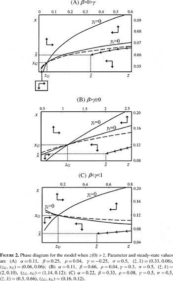
Figure 2 is a phase diagram in the (z, x) space when

. From (14a) the γ_z=0 locus, x=αz^β, is strictly increasing, strictly concave, and stable. From (14b), there are three possible shapes for the γ_x=0 locus, x=αz^β(β−γ)/(1−γ)+ρ/(1−γ). It is strictly decreasing and convex when γ>β, strictly increasing and concave when γ<β, and constant when γ=β. In any case, given (14b), the γ_x=0 locus is unstable and its slope is smaller than that of the γ_z=0 locus. The fulfilment of condition (11) entails

being below the γ_x=0 locus, because substituting

into the expression for the γ_x=0 locus yields

The γ_z=0 locus is strictly increasing with x→0 as z→0 and x→+∞ as z→+∞. The γ_x=0 locus is, in any case, above the γ_z=0 locus at least in a neighborhood of z=0 since x→ρ/(1−γ) as z→0. Hence, there is a unique positive state (z_G, x_G), which is a saddle point. If the γ_x=0 locus is increasing, it is flatter than the γ_z=0 locus. This implies that the stable saddle path must be strictly increasing and flatter than the γ_x=0 locus. Panel A in Figure 2 is a phase diagram in this case. If the γ_x=0 locus is strictly decreasing (constant), the stable saddle path is strictly decreasing (constant). Panel B in Figure 2 depicts a phase diagram in this case. The stable saddle paths are represented as dashed lines.

Phase diagram for the model when $z(0)\,{\gt}\,\hat{z}$. Parameter and steady-state values are (A) α=0.11, β=0.25, ρ=0.04, γ=−0.25, σ=0.5, $(\hat{z},\hat{x})\,{=}\,(0.33,0.06)$, (zG, xG)=(0.06, 0.06); (B) α=0.11, β=0.66, ρ=0.04, γ=0.3, σ=0.5, $(\hat{z},\hat{x})\,{=} (2,0.10)$, (zG, xG)=(1.14, 0.12); (C) α=0.22, β=0.33, ρ=0.08, γ=0.5, σ=0.5, $(\hat{z},\hat{x})\,{=}\,(0.5,0.66)$, (zG, xG)=(0.16, 0.12).

DECENTRALIZED ECONOMY

We now consider the representative agent in a decentralized economy. The agent maximizes his isoelastic utility function, (1), subject to the accumulation of physical capital,

where i is private investment, and the budget constraint

where agent's income, y, is given by (4), τ is the rate of income tax, and s is the agent's share of time-varying lump-sum taxes.

The government faces a balanced-budget constraint at each moment in time,

where S denotes aggregate lum-sum transfers. For simplicity, we do not explicitly consider financing by debt issue since, because of Ricardian Equivalence, the lump-sum tax is equivalent to debt when the sequence of fiscal parameters is held fixed. A constant consumption tax is not considered either, since it acts as a lump-sum tax in the absence of laborleisure choice in this model.

Let L be the current-value Lagrangian of the representative agent's problem, and let ν and μ be the multipliers for the constraints (15) and (16), respectively:

The first-order conditions are

plus the transversality condition

The nonnegativity constraint on private investment has been taken into account in equation (18b). These conditions are also sufficient since the current-value Hamiltonian, H=c^γ/γ+νi, and the constraints are jointly concave in the states and the controls.

In what follows, the equilibrium conditions y=Y, k=K, i=I, c=C are imposed. The aggregate resource constraint (8) can be derived from (16) and (17). Let x=C/K denote the ratio of consumption to private capital, z=K_g/K, the ratio of public to private capital, and g=G/Y, the ratio of public investment to output. The interior solution, when the nonnegativity constraint on private investment is nonbinding (i>0), can be easily obtained. Equation (18b) entails having ν=μ. From (18a) and (18c), we obtain the growth rate of consumption as

. Thus, the dynamics of the economy can be represented by the system

The steady state of this system is characterized by

, so that we obtain the following relationships, where tildes denote steady states:

For this system to have a feasible solution,

and

, the following condition must be met:

The transversality condition (18d) now requires

. This condition will surely be met when the policy parameters g and τ are chosen optimally so as to replicate the first-best equilibrium of the centrally planned economy (see Section 5).

The local saddle-path stability of system (19) can be readily established. Linearizing the dynamic system (19) about the steady state yields

The determinant of the coefficient matrix A can be computed as

Since det(A)<0, matrix A has one unstable eigenvalue and one stable eigenvalue, and so, the steady state is locally saddle-path stable.

If the constraint on nonnegative private investment is binding, i=0, we simply have that C=(1−g)αK^β_gK^1−β. Thus, the dynamics of the economy can be represented by

OPTIMAL FISCAL POLICY

In this section, we determine the fiscal policy that will enable the decentralized economy to attain the first-best equilibrium of the centrally planned economy. First, we compute the optimal policy in the steady state when

. In this case, comparing (10a)–(10b) with (20a)–(20b), and substituting

from (10c), we see that the steady-state equilibrium values of the centrally planned economy,

, and the market economy,

, will coincide if and only if the tax rate on income τ satisfies

or, equivalently,

The optimal tax rate on income is clearly feasible as 0[les ]τ<1. The intuition for the tax rate on income (24) is straightforward. This choice of the tax rate equates the social return to private capital accumulation, (1−β)αz^β, with the after-tax private rate of return, (1−τ)(1−βσ)αz^β. Having set the distortionary income tax in an optimal manner, lump-sum taxes (or, equivalently, consumption taxes and/or debt) should be set so as to satisfy the government budget constraint (17).

The effect of congestion on the optimal tax rate on income can be ascertained by noting that

which means that the higher the value of σ, the lower the congestion, and the lower the optimal tax rate on income. If there is no congestion, σ=1, the optimal tax rate on income is zero, τ=0. In this case, there is no externality, and so, capital income should be untaxed. The first-best optimum requires the use of lump-sum taxation (or, equivalently, consumption taxation and/or debt) to finance public investment. If congestion is proportional, σ=0, capital income should be taxed at a rate τ=β. Equation (10c) entails having

, and so, the government should impose an income tax in excess of its current investment costs, rebating the excess as lump-sum transfers. The idea that the presence of congestion favors an income tax over lump-sum taxation or consumption taxation has been shown by Barro and Sala-i-Martín (1992). In presence of proportional relative congestion, models in which government expenditure appears as a flow satisfy

, so that the expenditure is exactly self-financing. In the present case, because congestion in public capital enhances the return to private capital, a larger tax is required to offset this incentive to overaccumulate private capital.

If

, then I=0 and the first-best equilibrium is described by system (13) up to the point in which

. The corresponding system in the decentralized economy is (23). First note that Equations (13a) and (23b), which describe the dynamics of the ratio of public to private capital, z, in the centrally planned and decentralized economies, respectively, coincide after substituting the optimal value of g=1−x/(αz^β) in (23a). Thus, the first-best equilibrium can be achieved by setting the optimal share of government to output equal to g=1−x/(αz^β), where

and can be sustained by any combination of income taxation and lump-sum taxation that satisfies the government budget constraint (17), up to the point at which

. After that, the economy reaches its steady-state value given by (10), the tax rate on income should be set at the value given in (24), and the public investment share of output should be set at the value

given in (10c).

If

, then G=0 and the first-best equilibrium is described by system (14) up to the point at which

. The corresponding system in the decentralized economy is (19). First note that Equations (14a) and (19a), which describe the dynamics of the ratio of public to private capital, z, in the centrally planned and decentralized economies, respectively, coincide after substitution of the optimal value of g=0. Comparing (14b) and (19b) with g=0, we see that the decentralized economy will fully replicate the dynamic path of x in the optimal solution if and only if the tax rate on income is set according to (24), that is, τ=β(1−σ)/(1−βσ). Thus, the tax revenue must be rebated as lump-sum transfers to consumers in order for the government budget constraint (17) be met, up to the point at which

. After that, the economy stays at its steady-state value given by (10), the tax rate on income must be kept at its value given in (24), and the public investment share of output must be set at the value

given in (10c).

COMPUTATION OF THE FIRST-BEST EQUILIBRIUM

In this section, we indicate how the first-best equilibrium can be computed. We first show how the Turnovsky (1997) model relates to the one-sector endogenous growth model with physical and human capital analyzed by Barro and Sala-i-Martín (1995). Thereafter, we consider the determination of the transitional path.

Barro and Sala-i-Martín (1995, Ch. 5) analyze the one-sector model with physical and human capital. In this model, output is produced with the Cobb-Douglas production function Y=αH^βK^1−β, 0<β<1, where K is physical capital and H is human capital. The economy's resource constraint is Y=I_K+I_H+C, where I_K and I_H are gross investment in physical and human capital, respectively, which must each be nonnegative, and the stocks of physical and human capital evolve according to the dynamic equations

and

, respectively.

It can be readily noted that the one-sector model with physical and human capital and Turnovsky (1997) model coincide if human capital is identified with public capital, so that H≡K_g and I_H≡G, capital stocks do not depreciate (δ=0), and there is no congestion (σ=1). Barro and Sala-i-Martín (1995, pp. 202–203) claim that during the transition the economy will be on the stable saddle path corresponding to the system that describes the dynamics of the economy as long as the constraint on nonnegative investment in one of the factors is binding (see also their Figures 5.10 and 5.11).

Thus, it may be expected that the Barro and Sala-i-Martín analysis of the transitional dynamics of the one-sector model applies to the Turnovsky model as well, in particular, the fact that the transition path is on the stable saddle path of the system that describes the dynamics of the economy as long as the constraint on nonnegative investment in public or private capital is binding. We show that this procedure is generally incorrect because the economy does not have to evolve along the stable saddle path of system (13) or (14). First, we prove the continuity of the optimal consumption path.

PROPOSITION 1. The path of consumption is continuous on the optimal solution.

Proof. We have shown that one of the nonnegativity restrictions on investment in public or private capital is never binding. Hence, equations (9b) and (9c) entail having λ(t)=ν(t) [if

] or λ(t)=μ(t) [if

] at any time. The continuity of the shadow prices ν(t) and μ(t) require that λ(t) be continuous as well. The continuity of the consumption path C(t) follows then from equation (9a).

We now show that the economy does not have to evolve along the stable saddle path of system (13) or (14), as the case may be that describes the dynamics of the economy as long as the constraint on nonnegative investment in one of the types of capital is binding, in the direction of the “hypothetical target,” z_I or z_G, respectively, up to the point where z reaches its steady-state value

.

PROPOSITION 2. If

and (i) 0[les ]γ<β or (ii) 0<β=γ or (iii) β<γ<1, the transition path cannot be on the stable saddle path of the system that describes the dynamics of the economy as long as the constraint on nonnegative investment in one of the factors is binding.

Proof.

1. If γ<β, the γ_x=0 locus is strictly increasing and the stable saddle path is strictly increasing and flatter than the γ_x=0 locus. Therefore, it must be above x_G to the right of z_G. Since
   , the condition (11) and γ[ges ]0 entail having
   . As
   , this implies that the steady state
   must be below the stable saddle path of system (14). Panel (B) in Figure 2 illustrates this case.
2. If 0<γ=β, then
   . Now, the stable saddle path is constant, and so, it must be above
   .
3. If β<γ<1, then the γ_x=0 locus is decreasing and is above
   . The stable saddle path slopes downward and is above the γ_x=0 locus. Hence,
   and the stable saddle path are in distinct regions of the phase diagram. Panel (C) in Figure 2 illustrates this case. In any case, the result follows from the continuity of x(t) on the optimal solution.

Proposition 2 is not exhaustive in the sense that even if the conditions do not apply, the transition path may still be off the stable saddle path of the system that describes the dynamics of the economy as long as the constraint on nonnegative investment in one of the types of capital is binding. If

or

and β>0>γ, Figure 1 and Panel (A) of Figure 2, respectively, depict numerical examples that show that the steady state

does not have to be on the stable saddle path of the initial dynamical system in each of these cases for the parameter values quoted. The stable saddle paths have been computed by means of the time elimination method [Mulligan and Sala-i-Martín (1993)] and are represented as dashed lines.

Since the state variables K(t) and K_g(t) are continuous, the ratios z(t) and, as a result of Proposition 1, x(t) must be continuous as well. Furthermore, the economy's resource constraint implies that I(t)+G(t) must be continuous although I(t) and G(t) can jump (as they do in effect). According to Proposition 1, when the ratio of public to private capital, z, reaches its steady-state value,

, the ratio of consumption to physical capital x must also reach its steady-state value,

, with no jump.

We now explain how the transitional path can be computed. Suppose that

. In the interval [0, T] the dynamics of the economy are described by system (13). At time T the economy reaches its steady state when, as the paths of z and x are continuous,

and

. Note that at this stage the time T is unknown. Thus, the time paths of z and x in [0, T] and the time T can be obtained by solving the dynamical system

with initial condition z(0)=K_g(0)/K(0)=z₀, and terminal conditions

and

. From time t=T on, we have

and

. The time elimination method [Mulligan and Sala-i-Martín (1993)] is a simple and efficient numerical technique that can be used to compute the transitional path. The policy function x(z) can be computed by solving the initial-value problem,

The free final time boundary problem has been transformed in an initial-value problem in which time does not appear. Note that the slope of the policy function is never undefined since γ_z>0 along the transition to the balanced growth path. Standard numerical methods can be used to solve this first-order differential equation in z. For instance, we have used the Mathematica ν4.1 command NDSolve to compute the policy function depicted in Figure 1. Once the policy function x(z) has been computed, time must be reintroduced. The time path of z can be computed by solving the initial-value problem,

Then, we compute the time T at which

. From time t=T on, the optimal path is

. The time path of x can be obtained by substituting the optimal time path z(t) into the policy function x(z) in [0, T], x(t)=x(z(t)). From time t=T on, we have

. The time paths determined in this manner are clearly continuous. Once the paths of z and x have been computed, the time paths of the remaining variables can be readily obtained [see Mulligan and Sala-i-Martín (1993)].

If

, the transitional dynamics can be determined in a similar manner. The method described above has been used to compute the policy functions depicted in Figure 2.