ORIGINS AND EARLY DEVELOPMENT OF THE MMM

In the early 1970's, the structural econometric modeling, time-series analysis (SEMTSA) approach that provides methods for checking existing dynamic econometric models and for constructing new econometric models was put forward; see Zellner and Palm (1974, 1975, 2004), Palm (1976, 1977, 1983), and Zellner (1997, p. IV; 2004). In Zellner and Palm (2004), many applications of the SEMTSA approach are reported, including some that began in the mid-1980's that involved an effort by Garcia-Ferrer, Highfield, Palm, Hong, Min, Ryu, Zellner, and others to build a macroeconometric model that works well in explaining the past, prediction, and policymaking. In line with the SEMTSA approach, we started the model-building process by developing dynamic equations for individual variables and tested them with past data and in forecasting experiments. The objective is to develop a set of tested components that can be combined to form a model and to rationalize the model in terms of old or new economic theory.

The first variable that we considered was the rate of growth of real gross domestic product (GDP). After some experimentation, we found that various variants of an AR(3) model, including lagged leading indicator variables—namely the rates of growth of real money and of real stock prices—called an autoregressive-leading indicator (ARLI) model worked reasonably well in point forecasting and turning point forecasting experiments using data first for 9 industrialized countries and then for 18 industrialized nations. Later, a world income variable, the median growth rate of the 18 countries' growth rates was introduced in each country's equation and an additional ARLI equation for the median growth rate was added to give us our ARLI/WI model. The variants of the ARLI and ARLI/WI models that we employed included fixed-parameter and time-varying parameter state-space models. Further, Bayesian shrinkage and model-combining techniques were formulated and applied that produced gains in forecasting precision. See Zellner and Palm (2004) and Zellner (1997, p. IV) for empirical results. It was found that use of Bayesian shrinkage techniques produced notable improvements in forecast precision and in turning-point forecasting with about 70% of 211 turning-point episodes forecasted correctly; see Zellner and Min (1999).

Given these ARLI and ARLI/WI models that worked reasonably well in forecasting experiments using data for 18 industrialized countries, the next step in our work was to rationalize these models using economic theory. It was found possible to derive our empirical forecasting equations from variants of an aggregate demand and supply model in Zellner (2000). Further, Hong (1989) derived our ARLI/WI model from a Hicksian IS-LM macroeconomic theoretical model while Min (1992) derived it from a generalized real-business-cycle model that he formulated. Although these results were satisfying, it was recognized that the root mean squared errors of the models' forecasts of annual growth rates of real GDP, in the vicinity of 1.7 to 2.0 percentage points, while similar to those of some OECD macroeconometric models, were rather large. Thus, we thought about ways to improve the accuracy of our forecasts.

In considering this problem, it occurred to us that perhaps using disaggregated data would be useful. For an example illustrating the effects of disaggregation on forecasting precision, see Zellner and Tobias (2000). The question was how to disaggregate. After much thought and consideration of ways in which others, including Leontief, Stone, Orcutt, the Federal Reserve-MIT-PENN model builders, had disaggregated, we decided to disaggregate by industrial sectors and to use Marshallian competitive models for each sector. In earlier work by Veloce and Zellner (1985), a Marshallian model of the Canadian furniture industry was formulated to illustrate the importance of including not only demand and supply equations in analyzing industries' behavior but also an entry/exit relation. It was pointed out that on aggregating supply functions over producers, the industry supply equation includes the variable, the number of firms in operation at time t, N(t). Thus, there are three endogenous variables in the system, price p(t), quantity q(t), and N(t), and, as Marshall emphasized, the process of entry and exit of firms is instrumental in producing a long-run, zero-profit industry equilibrium. Further, given that producers were assumed to be identical, profit maximizers with Cobb-Douglas production functions and selling in competitive markets with “log-log” demand functions and a partial-adjustment entry/exit relation, it was not difficult to solve the system for a reduced-form equation for industry sales. As will be shown below, this system yielded a reduced-form logistic differential equation for industry sales, including a linear combination of “forcing” variables, namely, rates of growth of exogenous variables that affect demand and supply (e.g., real income, real factor prices and real money).

Given this past work on a sector model of the Canadian furniture industry, it was thought worthwhile to consider similar models, involving demand, supply, and entry/exit relations for various sectors of the U.S. economy, namely, agriculture, mining, construction, durables, wholesale, retail, etc., and to sum forecasts across sectors to get forecasts of aggregate variables. Whether such “disaggregate” forecasts of aggregate variables would be better than forecasts of the aggregate variables derived from aggregate data was a basic issue. Earlier, these aggregation/disaggregation issues had been considered by many, including Zellner (1962), Lütkepohl (1986) and de Alba and Zellner (1991), with the general analytical finding that many times, but not always, it pays to disaggregate. In addition, we were quite curious about whether inclusion of entry/exit relations in our model that do not appear generally in other macroeconomic models would affect its performance.

To summarize some of the positive aspects of disaggregation by sectors of an economy, note that these sectors, for example, agriculture, mining, durables, construction, and services, exhibit very different seasonal, cyclical, and trend behavior and that there is great interest in predicting the behavior of these important sectors. Further, sectors have relations involving both sector-specific and aggregate variables, with the sector-specific variables (e.g., prices, weather) giving rise to sector-specific effects. Since sector relations have error terms with differing variances and that are correlated across sectors, it is possible not only to use joint estimation and prediction techniques to obtain improved estimation and predictive precision but also to combine such techniques with the use of Stein-like shrinkage techniques to produce improved estimates of parameters and predictions of both sector and aggregate variables. In the literature, such approaches have been implemented successfully using time-varying parameter, state-space models to allow for possible “structural breaks” and other effects leading to parameters' values changing through time. See, Zellner et al. (1991) and Quintana et al. (1997) for examples of such applied analyses, the former in connection with predicting output growth rates and turning points in them for 18 industrialized countries and the latter in connection with formation of stock portfolios utilizing multivariate state-space models for individual stock returns, predictive densities for future returns, and Bayesian portfolio formation techniques.

To illustrate some of the points made in the preceding paragraph, in Figure 1, taken from Zellner and Chen (2001), the annual output growth rates of 11 sectors of the U.S. economy, 1949–1997, are plotted. It is evident that sectors' growth rates behave quite differently. For example, note the extreme volatility of the growth rates of agriculture, mining, durables, and construction; see the box plots presented in Zellner and Chen (2001, Fig. 1C) paper for further evidence of differences in dispersion of growth rates across sectors. Also, it is clearly the case that sector output growth rates are not exactly synchronized. With such disparate behavior of growth rates of different sectors, much information is lost in using aggregate data and models for forecasting and policy analysis.

U.S. sectoral real output growth rates.

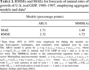
In Table 1, MAEs and RMSEs of forecast are presented for AR(3) and Marshallian macroeconomic models (MMMs) implemented with aggregate data. The AR(3) model has previously been employed as a benchmark model in many studies. In this case, in forecasting annual U.S. rates of growth of real GDP, 1980–1997, with estimates updated year by year, the MAE = 1.71 percentage points and the RMSE = 2.32 percentage points, both considerably larger than similar measures for the reduced-form equation of an aggregate MMM model, namely MAE = 1.48 and RMSE = 1.72. This improved performance associated with the MMM aggregate model flows from the theoretical aspects of the MMM model that led to incorporation of level variables and leading indicator variables (e.g., money and stock prices) in the reduced-form equation for the annual growth rate of real GDP.

Table 2 displays the effects of disaggregation on forecasting precision. When AR(3) models are employed for each of 11 sectors of the U.S. economy and SUR techniques are employed for estimation and forecasting, the MAE = 1.52 percentage points and RMSE = 2.21, both slightly below those obtained using an AR(3) model implemented with aggregate data shown in Table 1. However, on using reduced-form sector output growth rate equations associated with demand, supply, and entry/exit relations for each sector and SUR estimation and forecasting techniques, one-year-ahead forecasts of the outputs of each sector were obtained and totaled to provide forecasts of next year's total real GDP and its growth rate. It was found that the MAE = 1.17 percentage points and the RMSE = 1.40, both of which are considerably smaller than those for the MMM aggregate forecasts, MAE = 1.48 and RMSE = 1.72 and for the AR(3) model. Thus, in this case, use of the MMM's theory along with disaggregation has resulted in improved forecasting performance. For more results based on other methods and variants of the MMM, see Zellner and Chen (2001).

These positive empirical results encouraged us to proceed to analyze the properties of our models further and to add factor markets and a government sector to close the model. Further, we discovered that discrete versions of our MMM are in the form of chaotic models that, as is well known, have solutions with a wide range of possible forms, depending on values of parameters and initial conditions.

DEVELOPMENT OF A COMPLETE ONE-SECTOR MMM

In this section, we indicate how to formulate a complete one-sector MMM. Extending the work of Veloce and Zellner (1985) and Zellner (2001), we introduce demand, supply, and entry/exit equations. The supply equation is derived by aggregating the supply functions of individual, identical, competitive, profit-maximizing firms operating with Cobb-Douglas production functions. Further, firms' factor demand functions for labor and capital services are aggregated over firms to obtain market factor demand functions. Given a demand function for output and factor supply functions for labor and capital services, we have a complete one-sector, seven-equation MMM. Further, with the introduction of government and money sectors, an expanded one-sector MMM model with government and money is obtained and is described below. Results of some simulation experiments with these models are presented and discussed.

Product Market Supply, Demand, and Entry/Exit Equations

We assume a competitive Marshallian industry with N=N(t) firms in operation at time t, each with a Cobb-Douglas production function, q=A*L^αK^β, where A*=A*(t)=A_N(t)A_L(t)A_K(t), the product of a neutral technological change factor and labor and capital augmentation factors that reflect changes in the qualities of labor and capital inputs. Later, we introduce money services as another factor input. Additional inputs, for example, raw materials and inventory service inputs, can be added without much difficulty. The production function exhibits decreasing returns to scale with respect to labor and capital. This could be interpreted as the result of missing factors, for example, entrepreneurial skills that are not included in the model. Note that our Cobb-Douglas production function with decreasing returns to scale, combined with fixed entry costs introduced below, yields a U-shaped long-run average cost function. Given the nominal wage rate w=w(t), the nominal price for capital services r=r(t), and the product price p=p(t), and assuming profit maximization, the sector's nominal sales supply function is S=NAp^1/θw^−α/θr^−β/θ, where A=A*^1/θ, and 0<θ=1−α−β<1. On logging both sides of the equation for nominal sales S, and differentiating with respect to time, we obtain the industry nominal sales equation

where

. Note that with no entry or exit

and no technical change

, an equal proportionate change in the prices for product and for factors will not affect real sales. That is, from (1),

.

On multiplying both sides of the industry output demand function by p, we obtain an expression for nominal sales,

, where Y is nominal disposable income, H is the number of households, and the x variables are demand shift variables such as money balances, demand trends, etc. On logging and differentiating this last equation with respect to time, the result is

In a one-sector economy without taxes, we can replace nominal disposable income Y with nominal sales S. Ceteris paribus, an equal change in prices and nominal income will not affect real demand. That is, from (2),

, provided that η=η_s, implying no money illusion. Note that money illusion might arise from psychological reasons and/or systematic lack of information regarding relative prices and systematic errors in anticipations. Also, equation (2) can be expanded to include costs of adjustment, habit persistence, and expectation effects.

The following entry/exit equation completes the product market model:

with nominal profits given by Π=θS used in going from the first equality to the second in (3). Also in going from the first equality to the second, F=F(t)=F_e(t)/θ, with F_e(t) the equilibrium level of profits at time t taking account of discounted entry costs and γ=γ′θ, with γ=γ(t) and γ′=γ′(t). Such fixed costs make the long-run average cost function U-shaped for a firm operating with decreasing returns to scale, as assumed above. Equation (3), with γ=γ(t), where t is time, represents firm entry/exit behavior as a time-varying function of industry profits relative to the equilibrium level of profits. Further, equation (3) can be elaborated to take account of possible asymmetries, expectations, and lags in entry and exit behavior. For example, exit may not occur immediately if fixed costs incorporated in F_e are sunk.

Factor Market Demand and Supply Equations

Now we extend the model to include demand and supply equations for labor and capital. From assumed profit maximization, with N competitive firms operating with Cobb-Douglas production functions, as described above, the aggregate demand for labor input is L=αNpq/w=αS/w. Similarly, the aggregate demand for capital services is K=βNpq/r=βS/r. Logging and differentiating these last two equations with respect to time, we obtain

As regards labor supply, we assume

. Also, with respect to capital service supply, we assume

where the z and v variables are “supply shifters.” As before, we replace nominal income by nominal sales, and logging and differentiating with respect to time, we obtain

Above,

is the rate of change of the number of households.

The above seven-equation model is complete for the seven endogenous variables N, L, K, p, w, r, and S with the variables H, A*, γ′, F_e, x, z, and v assumed exogenously determined. The model can be solved analytically (see Appendix A for details) for the reduced-form equation for

that is given by

where a and b are parameters and g is a linear function of the rates of change of the exogenous variables given above. If a, b, F, and g have constant values, (8) is the differential equation for the well-known and widely used logistic function. Further, if g=g(t), a given function of time, as noted by Veloce and Zellner (1985, p. 463) the equation is a variant of Bernoulli's differential equation. Note that g may change through time because of changes in the rates of growth of technological factors, households, etc.; for an explicit expression for g(t), see equation (A.5) in Appendix A. Further, the logistic equation in (8) can be expressed as

where k₁=(g−γF)/(1−f) and k₂=−γ/(1−f).

The solution to (9) is given by

where c=(1+k₁/k₂S₀) with S₀ the initial value. Also, from (9), it is seen that there are two equilibrium values, namely, S = 0 and S=k₁/k₂, with the former unstable for positive values of the k parameters. Note that for constant values of the parameters, (9) cannot generate cyclical movements. However, if the parameters are allowed to vary, the output of (9) can be quite variable. Further, in some cases, there may be a discrete lag in (9) and then the equation becomes a mixed differential-difference equation that can have cyclical solutions; see, for example, Cunningham (1958). Whether the economy is best modeled using continuous-time, discrete-time, or mixed models is an open issue that deserves further theoretical and empirical attention.

The following are discrete approximations to equation (9) that are well known to be chaotic processes; see, for example, Day (1982, 1994), Brock and Malliaris (1989), Kahn (1989), and Koop et al. (1996). That is, the solutions to these deterministic processes, even with the parameters constant in value, can resemble the erratic output of stochastic processes. We have considered two discrete approximations to (9):

While the differential equation in (9) with constant parameters exhibits a smooth convergence to its limiting value, the processes in (10) and (11) can exhibit oscillatory behavior. Further, in computed examples, the paths associated with (10) and (11) differed considerably in many cases. For example, it was found that the equations in (10) and (11) gave rise to a smooth approach to an equilibrium value when 0<k₁<1 and k₂>0 and oscillatory approaches to equilibrium when k₁>1. See plots of solutions to (9), (10), and (11) in Figures 2 and 3 for different values of the parameter k₁. Note that (10) and (11) can yield quite different solutions for the same value of the parameter. Also, if the measured values of S have additive or multiplicative biases, the properties of (10) and (11) will be further affected. Last, note that since the coefficients of (9), (10), and (11) are functions of the rates of change of the exogenous variables, it is probable that they are not constant in value but vary with time. It is thus fortunate that data can be brought to bear on, for example, discrete versions of equation (8) that allow for variation in the exogenous variables; see, for example, Veloce and Zellner (1985) and Zellner and Chen (2001) for examples of such fitted functions. Also, discrete versions of the structural equation system presented above can be estimated using data.

Discrete approximations to the logistic equation: k1=1.93, k2=0.193, S0=0.5.

Difference equation (10): k1=2.8, k2=0.28, S0=0.5.

Various simulation experiments have been done with the seven-equation model described above that indicate that it can produce a rich range of possible solutions, depending on the values of parameters and properties of input variables. For example, in Figures 4–7 are shown the outputs of the seven-equation model under various conditions. In Figures 4 and 5, the paths of the nominal and real variables are shown when the model is started up at nonequilibrium initial values. Figures 6 and 7 show how shocks to demand and to factor supplies affect the system. In these continuous-time, differential equation versions of the model, the paths are relatively smooth and nonoscillatory, given that exogenous variables' paths are smooth. As was seen above and will be shown further below, discrete versions of the model can exhibit various types of oscillatory behavior.

Simulation of the one-sector model, nominal variables. Rates of growth of exogenous variables are assumed equal to zero.

Simulation of the one-sector model, real variables. Variables S, w, and r deflated by p (nominal), and there is zero growth in exogenous variables.

One-sector model (real variables), with demand shock from t=25 to t=30. Exogenous demand increases by 2% in periods 25 though 30 $(\dot {x}_i/x_i\,{=}\,0.02)$ Variables S, w, and r are deflated by p (nominal), and there is zero growth in other exogenous variables.

One-sector model (real variables), with labor supply shock from t=25 to t=30. Exogenous labor supply increases by 10% in periods 25 though 30 $(\dot {z}_i/z_i\,{=}\,0.1)$. Variables S, w, and r are deflated by p (nominal), and there is zero growth in other exogenous variables.

One-Sector Model with Government and Monetary Sectors

Now we shall add government and money sectors to the above model. We assume that government collects taxes and buys goods and services in both the final product market and in the market for factors of production. For simplicity, we assume that there are taxes on sales and corporate profits, an exogenously determined budget deficit or surplus and a fixed composition of government expenditure. To model the money market, we consider the services of money as a factor of production, demanded by firms and government. In addition, we assume that households demand money services, include money balances in the demand for final product and assume that the money supply is exogenously determined.

A discrete-time version of this expanded one-sector model that includes a money market and a government sector has been formulated; see Appendix B for its equations. It can be solved readily and has been employed in simulation experiments designed to study the impacts of changes in monetary policy, the corporate income tax, the sales tax, and the government deficit on other variables. See, for example, Figure 8 in which the effects of a decrease in the corporate profit tax rate from 40% to 20% are shown. It is seen that there are substantial increases in employment and output and reductions in government expenditures and receipts. In addition there is a large impact on the interest rate and smaller changes in factor prices and the price level.

Simulation of a corporate tax cut in the one-sector model. At period 25, the corporate tax rate drops from 0.4 to 0.2. Government expenditures are adjusted to government revenues, and there is zero growth in exogenous variables.

TWO- AND n-SECTOR MODELS

In addition to the one-sector MMM with a money market and a government sector, similar two- and n-sector models have been formulated and studied; see Appendix C for details. For such an n-sector model, there are 7n+12 equations. Thus, for n=1, there are 19 equations and for n=2, 26 equations, etc.

For the two-sector MMM, n=2, the 26 equations have been solved to yield the following equations for the sales and number of firms in operation for sectors 1 and 2:

where the coefficients, A, B, …, J are functions of lagged endogenous variables and rates of change of exogenous variables, and the gammas have constant values.

Simulation experiments using the nonlinear difference equations in (12)–(15) with constant parameters indicate that solutions can have a rich range of properties. For some examples, see Figures 9–13. In Figure 9, the variables, namely, numbers of firms in operation in the two-sectors and sales of the two-sectors follow rather smooth paths to their equilibrium values. However, with the parameter values used for the experiments described in Figure 10, the paths of the variables in the two sectors show systematic, recurrent, cyclical properties. In contrast to the relatively smooth and systematic features shown in Figures 9 and 10, with the parameter values employed in experiments reported in Figures 11–13, it is seen that various types of “bubbles and busts” behavior are exhibited by the two-sector MMM. It is thus apparent that this relatively simple model has a broad range of possible solutions, even when the rates of change of the exogenous variables are assumed to have constant values. Allowing for changes in the exogenous variables' growth rates of course enlarges the range of possible solutions to this two-sector model and MMMs containing more than two sectors.

Simulation for the two-sector model (smooth path), where A=G=−0.07, B=F=0.05, D=J=0.01, E=I=0.01, C=0.2, H=0.1, γ1=γ2=0.1, F1=F2=−2. Initial values are N01=N02=1, S01=S02=0.1. All coefficients are assumed constant.

Simulation for the two-sector model (cyclical path), where A=G=−0.08, B=F=0.06, C=H=0.2, D=J=0.01, E=I=0.01, γ1=γ2=0.1, F1=F2=−2. Initial values are N01=N02=1, S01=S02=0.1. All coefficients are assumed constant.

Simulation for the two-sector model (“bubbles and busts”), where A=G=−0.08, B=F=0.05, C=0.2, H=0.1, D=0.035, J=0.01, E=0.03 I=0.01, γ1=γ2=0.1, F1=F2=−2. Initial values are N01=N02=1, S01=S02=0.1. All coefficients are assumed constant.

Simulation for the two-sector model (“bubbles and busts”), where A=−0.07, G=−0.069988, B=0.0964, F=0.025, C=0.1, H=0.2, D=E=I=J=0.01, γ1=γ2=0.1, F1=F2=−2. Initial values are N01=N02=1, S01=S02=0.1. All coefficients are assumed constant.

Simulation for the two-sector model (“bubbles and busts”), where A=−0.08, G=−0.0208, B=F=0.09, C=0.1, H=0.2, D=0.035, E=0.0324872, I=J=0.01, γ1=γ2=0.1, F1=F2=−2. Initial values are N01=N02=1, S01=S02=0.1. All coefficients are assumed constant.

SUMMARY AND CONCLUSIONS

In this report, we have briefly reported our progress in producing one-, two- and n-sector versions of the MMM that are rooted in traditional economic theory and yet provide a rich range of possible forms that can be implemented with sector data. For example, Zellner and Chen (2001) implemented the MMM's reduced-form equations in forecasting 11 U.S. industrial sectors' annual outputs and their total using various estimation and forecasting techniques with encouraging results, as mentioned in Section 1. These results indicate that it pays to disaggregate to obtain improved forecasts of aggregate, real GDP growth rates as well as sector forecasts. Of course, such results may be improved by using the structural equations for sectors rather than just one reduced-form equation per sector.

Further, there are many ways to improve the “bare bones” MMMs that we presented above by drawing on the vast economic literature dealing with entry and exit behavior, anticipations, various industrial structures, alternative forms of production and demand relations, dynamic optimization procedures, introduction of stochastic elements, etc. In addition, there is a need to consider inventory investment, intermediate goods, vintage effects on capital formation, imports and exports, etc. Although the list of extensions is long, just as in the case of the Model T Ford, we believe that our MMM is a fruitful initial model that will be developed further to yield improved, future models in the spirit of Deming's emphasis on continuous improvement. Most satisfying to us is the fact that we have an operational, rich, dynamic “core” model that is rationalized by basic economic theory. This case of “theory with measurement” is, in our opinion, much to be preferred to “measurement without theory” or “theory without measurement.”

APPENDIX A. SOLUTION OF ONE-SECTOR MODEL FOR REDUCED-FORM EQUATION

In this appendix, we indicate how the seven-equation MMM in the text has been solved to yield the differential equation for sales, S(t), shown in equation (8) in the text. First, solve equations (4) and (6) for the rate of change of w,

:

Then solve equations (5) and (7) for the rate of change of r,

:

Further, from the product demand equation (2) in the text, we obtain

On substituting from (A.3) in (A.1) and (A.2) and then substituting from (3), (A.1), (A.2), and (A.3) in (1) and solving for

, the result is

where g represents a linear combination of the rates of growth of the exogenous variables, given by

and

Note that with η=η_s, that is, no money illusion, f=1 and (A.4) reduces to S=F−g/γ.

APPENDIX B. A DISCRETE-TIME ONE-SECTOR MMM WITH MONETARY AND GOVERNMENT SECTORS

In this MMM with monetary and government sectors, we assume that the government collects taxes, produces government output, and buys goods in the product market and factor services in the factor markets. For simplicity, we assume that the only taxes are taxes on sales and profits, an exogenously determined deficit/surplus and a fixed composition of government expenditures. Herein, we find it convenient to express the model in terms of discrete time and denote the rate of change of a variable, say X, from period t−1 to t as X_rt≡(X_t−X_t−1)/X_t−1.

Given profit maximization under competitive conditions, using a Cobb-Douglas production function, as above, but with the addition of a money service factor input, the nominal sales supply function, expressed in terms of rates of change, with the nominal interest rate representing the price for monetary services, is given by

where τ_rt is the rate of change of the nominal interest rate, λ is the exponent of money services in the production function, and 0<1−α−β−λ<1.

The demand function for the final product includes the rate of change of government expenditure on final product G_rgt, as well as a tax on nominal income. To obtain the rate of change in total sales S_rt, rates of change of governmental and private expenditures are weighted by their share in total expenditure at time t−1 as follows:

where T^s′_rt=(1+T^s_rt) with T^s_rt the rate of change of the sales tax. The rate of change of nominal government expenditures is given by G_rgt=G_rt, the rate of change in total government expenditures, defined below. Also, M_rht represents the rate of change of households' demand for real money balances, as discussed below.

The entry/exit equation in this discrete-time version of the model is an elaboration of that used in the continuous-time version, namely,

In (B.3), there is an allowance for corporate taxation on profits T^c_t−1, time-varying entry costs F_t−1 nominal sales deflated by the price level p_t−1, and entry costs deflated by a price index for the cost of factors p^l_t−1. Also, here firm entry is proportional to profits at the firm level and thus we divide the total sector's profits by the number of firms N_t−1.

Further, in this model we assume that government expenditure affects firms' productivity as shown in the expression for the technological change factor,

where G_rt−p_rt is the rate of change of real government expenditure and the b_rit variables are technology shift variables such as those described above in formulation of our initial model. The parameter ω_g reflects the impact of the rate of change of real government expenditure on the rate of change of the technological factor, A_rt′ perhaps the result of government-financed research since government expenditure does not include only expenditures on consumption goods but also expenditures that may affect firms' productivity by providing public services, infrastructure, and R&D.

For each factor market, the model includes firms' and government demand equations, a supply equation, and an equilibrium equation. The money market includes also a household demand equation. In terms of rates of change, firms' demands for labor and capital services are denoted by L_rft and K_rft, respectively. Since we fix the composition of government expenditure, the government's demands, L_rgt and K_rgt, equal the rate of change of government total expenditure minus the rates of change of the prices of factors, as shown below:

Firms and the government demand real money balances as a factor of production whereas households' demand for the services of real balance depends on the real interest rate τ_rt−p_rt, real income, the number of households, and other variables, denoted by y_rit, that shift households' demand for real money balances. The equations for money demand are

Discrete versions of labor and capital supply functions are

and

In terms of rates of change, the supply of real money balances equals the supply of nominal balances, assumed exogenously determined, corrected for the change in the price level; that is,

Equilibrium conditions for factor markets involve equating factor supplies to weighted firm, government, and household demands for factors as follows:

Government nominal revenues are given by R_t=S_t(T^s_t+T^c_tθ). By defining T*_t=(T^s_t+T^c_tθ), the rate of change of government revenue is given by

The rate of change in nominal government expenditure is assumed to be tied to tax revenues plus an exogenously determined deficit/surplus, denoted by Def_t (as a percentage of total revenues) as follows:

Finally, the price index for production costs is a weighted average of the prices of the three inputs, given by

The above equations constitute the MMM incorporating money and government sectors. Several simulation experiments have been performed using the above model to study its responses to changes in tax rates, money supply, etc., that indicate it is operational. See Figure 7 for the effects of a temporary labor supply shock. Also, since monetary balances enter the model as an additional input factor, the effects of a monetary expansion/contraction are analogous in certain respects to the effects of a shock to labor or capital supply, except for the fact that there are also demand effects resulting from an increase or decrease in money balances.

APPENDIX C. DISCRETE-TIME -SECTOR MMM WITH GOVERNMENT AND MONEY SECTORS

In this appendix, the one-sector model described in Appendix B is extended to n sectors. Although there are no intermediate products, the n sectors are related to each other through interdependent demand and supply relations in factor and product markets and are individually and jointly affected by government expenditures and taxes. That is, (i) there is competition in the market for final products and services with demand functions, shown in (C.2), that are functions of a vector of prices allowing for direct and indirect effects of price changes on individual sectors' demands and similarly with respect to industries' product supply and individuals' labor supply functions; (ii) there is competition in factor markets for labor, capital, and money services with interdependencies shown in demand and supply relations in equations (C.5–C.7); and (iii) the model allows the government to affect individual sectors through purchases of final products (see equations C.2), to provide services that affect sectors' productivity (equations C.4), demands for inputs (equations C.5–C.7) and by taxing (C.15). Thus, the model allows for many types of important interactions among individuals, economic entities, and government.

As in Appendix B, we denote the rate of change of the ith variable from period t−1 to t by a subscript rit, that is, X_rit≡[X_it−X_it−1]/X_it−1, where the subscript i denotes the ith sector. Nominal supplies for each sector's products, assuming use of Cobb-Douglas production functions and profit maximization under competitive conditions, are given by

The demand functions for final products include the rate of change of nominal government expenditure, as follows:

where G_rit=G_rt for i=1, 2, …, n and η_ij is the cross-price elasticity of demand for product i relative to product j.

Sectors are permitted to have different technologies and entry and exit conditions, and thus the following individual entry and technology equations are employed:

For each factor market, the model includes the demands from n sectors and government, a supply equation, and an equilibrium condition. The money market also includes household demand.