INTRODUCTION
This paper presents a computable general equilibrium model of endogenous (stochastic) growth and cycles that can account for two key features of the aggregate data: balanced growth in the long run and business cycles in the short run. The model is built on Schumpeter's idea that economic development is the consequence of the periodic arrival of innovations. There is growth because each subsequent innovation leads to a permanent improvement in the production technology. Cycles arise because innovations trigger a reallocation of resources between production and R&D.
It is generally accepted in the literature that innovations play an important role in long-run economic growth.1
For example, this idea lies in the basis of the models developed by Aghion and Howitt (1992), Grossman and Helpman (1991), Romer (1990), and Segerstrom (1991).
Empirical evidence also suggests that there is a link between R&D and business cycles. Kleinknecht (
1987) reports that the number of patents varies significantly over time. At the level of firms, Lach and Schankerman (
1989) find that R&D Granger-cause investment in physical capital after a short lag. Lach and Rob (
1996) report that a similar tendency is observed at the level of industry. Geroski and Walters (
1995) document a procyclical behavior of innovations in the United Kingdom. In particular, Geroski and Walters (
1995, p. 927) conclude: “the procyclical variations in innovation which we observe are, no doubt, an important contributor to the procyclical variation in productivity growth which has been widely observed.”
The idea that both growth and cycles are an outcome of innovative activity has been advocated in previous literature. The origins of growth and cycles have been related to an extensive search for new technology and further refinement of old technology [Jovanovic and Rob (1990)], to the discovery of new technology and its subsequent diffusion [Andolfatto and MacDonald (1998)], and to the discovery of new technology and a subsequent shift of resources from R&D to production [Bental & Peled (1996), Freeman et al. (1999)].
The literature, however, explains long waves in economic activity but not short waves. In particular, two models that are related to ours, presented by Andolfatto and MacDonald (1998) and by Freeman et al. (1999), do not produce fluctuations in business-cycle frequencies by construction. High-frequency fluctuations are missing in Andolfatto and MacDonald (1998) because technology improvements are large and rare, so that imitation is the main source of the economy's dynamics. To be more specific, their model is parameterized to account for six major technology innovations in the United States during 1946–1994—for example, the chemicals revolution and the electronics revolution. Freeman et al. (1999) interpret innovations as infrastructural projects that require large amounts of investments and long periods of development—for example, railroads or telegraph systems. The model generates cycles of a constant shape and a constant (presumably long) duration, which are not comparable to cycles in the data.
Our approach to modeling innovations differs from those presented in the literature in several aspects. First, in our model, the aggregate level of production technology is determined by three factors: intensity of research effort, the current level of technology and a random element that can be interpreted as luck. Because of the presence of aggregate uncertainty, our model is capable of producing stochastic cycles that are similar to those generated by a typical real-business-cycle (RBC) model. In contrast, the previous literature has no uncertainty at the aggregate level, so that cycles are deterministic.2
In Andolfatto and MacDonald (1998), there is idiosyncratic uncertainty but not aggregate uncertainty; this is because a continuum of agents is assumed and thus the law of large numbers applies. In Freeman et al. (1999), uncertainty is absent: innovation occurs with the probability 1 as soon as the required amounts of R&D resources have been collected.
Concerning our assumption of the randomness of innovations, research projects clearly differ. Certain projects, such as the construction of railroads or telegraph systems, can generally be planned from the outset. Other projects may have highly uncertain outcomes, for example, the development of a treatment for cancer. Furthermore, research in new directions is typically preceded by trial and error, and many discoveries are purely accidental.
3 Jovanovic and Rob (1990) provide many examples of research projects that have had random outcomes.
Second, in our economy, technology increases in discrete increments of a fixed size, so that the economy experiences switches in regime, between positive growth and no growth at all.4
There is evidence that supports the two-regime process assumption. Hamilton (1989) finds that the periodic shifts between positive and negative growth in output concur remarkably with the dates of expansions and recessions in the U.S. economy.
Unlike the previous literature, we consider technological improvements to be relatively small and frequent. In our view, the development of a railroad system is not merely one great project, but rather a series of small projects: Productivity does not increase very much after the entire railroad has been constructed, but rather, productivity increases step-by-step as each phase of the railroad is completed and put into operation. Likewise, we do not think that either development or diffusion of the IBM PC-XT has led to an information revolution. Rather, we believe that productivity has increased, step-by-step, after the introduction of IBM's PC-286, -386, -486, etc.
5 A related idea appears in Jovanovic and Lach (1997, p. 7) in a context of a product-innovation model: “more important products are the embodiment of a larger number of innovations, so that, for example, the computer embodies a large ‘bunch’ of smaller innovations.”
As the consequence of frequent innovation, we obtain short waves of economic activity.
Finally, we differ from the literature in our methodology for the numerical study. To be specific, we do not try to distinguish from the data particular technology shocks to parameterize the model, but calibrate the model to reproduce the selected first moments of the aggregate series, as is typically done in RBC models. We subsequently test the validity of the model's predictions by looking at the second moments of the simulated series.
The main implications of our analysis are as follows: By construction, the model produces a balanced growth path, such that all the model's variables (except that of working hours) grow at the same constant rate in the long run. In the short run, the model generates random cycles that resemble business-cycle fluctuations in actual economies. The quantitative implications of the calibrated version of our model are very similar to those of Kydland and Prescott's (1982) model. Moreover, under some parameterizations, our model can correct two shortcomings of RBC models: it can account for the persistence in output growth and the asymmetry of growth within the business cycle.
This paper is organized as follows: Section 2 describes the model, derives the optimality conditions, and discusses some of the model's implications for growth and cycles. Section 3 outlines the calibration procedure and analyzes the quantitative implications of the model. Section 4 concludes.The appendices expose supplementary results. Appendix A decentralizes the planner's economy. Appendix B proves Proposition 1. Appendices C and D elaborate the calibration and solution procedures, respectively.
THE MODEL
In this section, we formulate the model and discuss some of its implications. We restrict our attention to a socially optimal economy. A competitive equilibrium version is discussed in Appendix A.
The Growing Economy
Time is discrete and the horizon is infinite, t∈{0, 1, …}. Output is produced according to the Cobb-Douglas production technology, Kαt−1N1−αt, α∈(0, 1), where the two inputs Kt−1 and Nt are physical capital and efficiency labor, respectively. The amount of efficiency labor is given by the product of the current labor productivity, At, and the aggregate physical hours worked, nt; that is, Nt=At·nt.
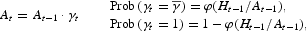
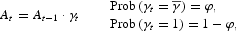
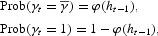
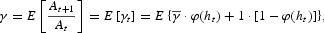
There is endogenous labor augmenting technological progress. In each period t, depending on a random draw, labor productivity either increases by a factor
; that is,
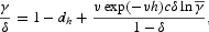
, or remains unchanged, At=At−1. The probability of innovation, φt, is endogenous: It depends on the human capital stock, Ht−1, and productivity, At−1.6
Thus, production technology follows a random-walk type of process. In
, where the probabilities of the two states, φt and (1−φt), change over time. The assumption of a random-walk process for innovations is in agreement with the data [see Geroski and Walters (1995)].
We assume that the probability function is homogeneous of degree zero and, thus, can be written as φ
t=φ(
Ht−1/
At−1). Moreover, we assume that φ(
x) is strictly increasing and strictly concave for all
x[ges ]0 and satisfies φ(0)=0 and lim
x→∞φ(
x)=1. The assumption of strict concavity of the probability function implies that there is a decreasing rate of return on human capital (in terms of the probability of innovation) in a given period. Furthermore, since the probability function is strictly decreasing in
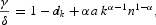
At−1, the rate of return on human capital also decreases across periods, as the economy develops. Therefore, to achieve continuous technological progress, human capital stock must grow at an average rate that is not lower than that of labor productivity. As we will show, under the assumption of a homogeneity of degree zero of the probability function, the economy follows a balanced growth path such that not only human capital but also output, consumption, and physical capital all grow at the same average rate as labor productivity does.
7 Consequently, our model reproduces empirical evidence that indicates that real economies constantly increase their spending on R&D, although their growth rates change relatively little. This evidence is documented by Coe and Helpman (1995), Griliches (1988), Grossman and Helpman (1991, Table 1.1), Jones (1995), and Kortum (1997), among others. Jones (1995) argues that such evidence cannot be replicated under the assumption of constant returns to R&D activity that is standard for R&D-based models; see, for example, Aghion and Howitt (1992), Grossman and Helpman (1991), and Romer (1990).
Note that, in our economy, human capital, Ht, is used exclusively for making innovations, that is, for R&D activity. We interpret human capital stock as a collection of all nonhuman and human resources that encourage innovation, that is, computers and other lab equipment in the R&D sector, a stock of knowledge of researchers, and all or a part of resources employed in the educational sector. Furthermore, we assume that human capital is one of the uses of output, that is, that it is produced by using the same technology as that used for producing consumption and physical capital.
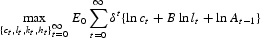
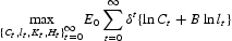
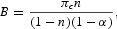
The planner maximizes the expected discounted lifetime utility of the representative consumer,
subject to
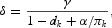
with initial condition (K−1, H−1, A−1) given. Here, E0 denotes the expectation, conditional on the information set in the initial period, δ∈(0, 1) is the discount factor, B is a positive constant, Ct and lt denote consumption and leisure, respectively; the agent's total time endowment is normalized to 1, that is, nt=1−lt; and finally, dk∈(0, 1] and dh∈(0, 1] are the depreciation rates of physical and human capital, respectively.
An equilibrium is defined as a sequence of contingency plans for an allocation {Ct, lt, Kt, Ht}∞t=0 that solves the utility maximization problem (1)–(3). All equilibrium quantities are restricted to being nonnegative and, in addition, leisure is assumed to satisfy lt[les ]1 for all t.
Relation to Kydland and Prescott's (1982) Model: Exogenous Growth and Cycles
By appropriately redefining the process for innovations, we can cast the model (1)–(3) into the standard neoclassical growth setup with exogenous growth and cycles. Indeed, assume that labor productivity (technology) in our model, At, is determined exogenously and does not depend on the human capital stock:
where φ∈[0, 1] is a constant. Because the probability of innovation is now fixed, both growth and cycles depend entirely on luck. Since human capital is useless now, the optimal choice of the planner is Ht=0 for all t, which takes us back to the familiar Kydland and Prescott (1982) model. Hence, an “exogenous stochastic growth and cycles” variant of the model (1)–(3) can be obtained by parameterizing Kydland and Prescott's (1982) model by the two-shock process (4).
To cast our model into the standard Kydland and Prescott's (1982) setup, we assume that growth is deterministic and cycles are stochastic by considering the following process for technology:
where θt is an exogenous technology shock following a first-order Markov process ln θt=ρln θt−1+εt with ρ∈[0, 1) and εt∼N(0, σ2), and Xt is exogenous labor-augmenting technological progress, Xt=X0γtx with X0∈R+ and γx[ges ]1.
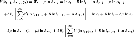
The Stationary Economy
Although the model formulated in Section 2.1 is nonstationary, it can be converted into a stationary model by using the appropriate change of variables. Let us introduce ct≡Ct/At−1, kt−1≡Kt−1/At−1, ht−1≡Ht−1/At−1. In terms of these variables, the problem (1)–(3) can be rewritten as follows:
subject to
where At=At−1·γt, and initial condition (k−1, h−1, A−1) is given.
The above transformation does not remove the growth completely: The growing-over-time endogenous technology At−1 is still present in the objective function (6).8
The standard transformation for removing the growth in Kydland and Prescott's (1982) model is ct≡Ct/Xt and kt≡Kt/Xt. The objective function obtained after this transformation contains the growing term Xt. However, in contrast to our model, the growing term in this case is exogenous and does not affect the equilibrium allocation.
It turns out, however, that a Markov (recursive) equilibrium exists, such that the corresponding optimal decision rules depend only on a current realization of
, but not on the growing term At−1. Moreover, such an equilibrium is unique. These results are formally established in the proposition below.
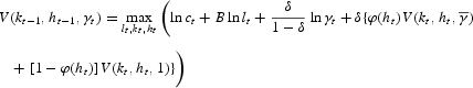
PROPOSITION 1(a). The optimal value function V for the problem (6)–(8) is a solution to the Bellman equation
subject to (7), (8).
(b) The Bellman operator is a contraction mapping.
proof. See Appendix B.
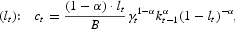
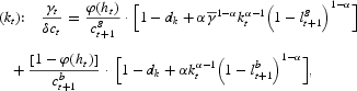
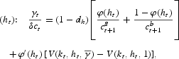
With interior equilibrium, a solution to the problem (9) satisfies first-order conditions (FOCs):
where the superscripts {g, b} correspond to the states
and γt=1, referred to as “good” and “bad” states, respectively.
In our model, the FOCs regarding leisure and physical capital are similar to the corresponding optimality conditions in the two-shock variant of Kydland and Prescott's (1982) model. However, in Kydland and Prescott's (1982) setup, the probabilities of states are determined exogenously by the assumed process for shocks, whereas, in our case, they are determined endogenously by the FOC with respect to human capital. When human capital is chosen in our economy, the planner takes into account that each additional unit of ht increases the probability of technological advancement, which, if it occurs, increases the lifetime utility by the amount
.
Endogenous Growth and Cycles
We have shown that, under the recursive formulation, a solution to the model with growth, {Ct, Kt, Ht}∞t=0, can be subdivided into two components: a growing-over-time stochastic trend, {At}∞t=0; and a solution to the stationary model, {ct, kt, ht}∞t=0. These two components can be interpreted as long-term growth and the short-term cyclical fluctuations, respectively. In our model, growth and cycles are endogenous in the sense that they depend not only on luck but also on the actions of the planner, that is, on the choice of human capital. [In Section 2.2, we have argued that the “exogenous growth and cycles” variant of our model coincides with Kydland and Prescott's (1982) model parameterized by the two-shock process (4)].
Fluctuations in our model take the form of cycles of a random length and shape and occur because technology's progress is stochastic. The cyclical ature of fluctuations is a consequence of the existing trade-off between production on the one hand and technological progress on the other. Specifically, a technological advance increases the rate of return on physical capital relative to that on human capital. This leads to a reallocation of resources from R&D to production and, as a result, lowers the probability of technological advance during the next period. In subsequent periods, the resources are gradually shifted back to R&D until the next technological advance occurs, and so on. In Section 3, we plot cycles produced by a calibrated version of the model.
The long-run growth is also due to technological progress. The model predicts that the economy follows a balanced growth path such that consumption and both capital stocks, {Ct, Kt, Ht}∞t=0, grow at the same stochastic rate γt while labor, {nt}∞t=0, and leisure, {lt}∞t=0, exhibit no long-run growth. The fact that the process for {ht}∞t=0 is stationary implies that the processes for the probability of innovation and the growth rate are also stationary. The expected growth rate in our economy is
where E is the unconditional expectation. Note that if parameters are chosen so that the average growth rate γ in our model is equal to the deterministic growth rate γx in Kydland and Prescott's (1982) model under (5), both models imply a similar balanced growth path. However, in our model, the time trend is stochastic, whereas in Kydland and Prescott's (1982) model, it is deterministic.
QUANTITATIVE ANALYSIS
In this section, we outline the calibration procedure and discuss simulation results. More details on the calibration procedure and the solution algorithm are provided in Appendixes C and D, respectively.
Calibration
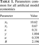
A distinctive feature of our endogenous-growth-and-cycles model is that it can be calibrated in the standard way employed in the RBC literature. Specifically, we choose the values of the parameters so that, in the steady state, the model reproduces the following statistics for the U.S. economy: the capital share in production α, physical-capital-to-output ratio πk, consumption-to-output ratio πc, average working time n, and average growth rate γ.9
Here, and further on in the text, z denotes the steady-state value of a variable zt.
We take the model's period as one quarter. We choose the values of α, π
k, and γ in line with the estimates presented by Christiano and Eichenbaum (
1992). We take the value of π
c, which is somewhat higher than it was in their paper, because our model does not contain the government. We borrow the value of
n from the micro study presented by Juster and Stafford (
1991). The above parameters are fixed for all simulations; they also identify the parameter
B in the utility function.
Table 1 summarizes the parameter choice.
We assume that the probability function is of the Poisson type
Furthermore, we assume that the depreciation rates of physical and human capital are equal. Under the above assumptions, we can uniquely determine the rest of the model's parameters,
, by fixing a human-capital-to-output ratio, πh. The empirical value of this ratio depends significantly on whether the variable ht is interpreted only as a stock of R&D expenditure or as a stock of both R&D and educational expenditure. During the period 1985–1995, the expenditure on R&D in the United States, amounted to 2.5%; of GDP, whereas the expenditure on education was 6.7%; and 5.4%; of GDP in 1980 and 1996, respectively.10
We consider four alternative values of the parameter π
h, such that π
h/π
k≡
h/
k∈{0.3, 0.4, 0.5, 0.6}. As is seen from
Table 2, these values imply the steady-state shares of human capital investment to output,
ih/
y, ranging from 6.34%; to 9.83%;, which is grossly consistent with the amount of expenditures on R&D and education in the U.S. economy.
11 The estimates of McGrattan and Prescott (2000) offer an alternative justification for the assumed range of h/k. This paper reports a ratio of approximately 0.6 between what they call unmeasured and measured corporate capital, with the former kind of capital being defined as brand names, patents, and firm-specific human capital.
In Table 2, we provide the values of the parameters
computed by our calibration procedure for each considered value of h/k. The parameters δ, dh, and dk decrease with πh, which can be seen from formulas (C.8) and (C.9) in Appendix C. The regularities that
increases with πh and that v decreases with πh are more difficult to understand, because the calibration of the parameters
and v requires finding a numerical solution to a nonlinear equation (C.11) and combining several conditions, such as (C.10), (C.12), and (C.13) (see Appendix C). However, one can gain a simple intuition about the implied inverse relation between the frequency and size of the innovations by looking at formula (13). In each of the cases considered, the model is calibrated to reproduce the average growth rate of output in the U.S. economy, γ. The result is that if technology improvements are small (large), they occur often (rarely). The quantitative expression of this effect is very significant: As the value of h/k rises from 0.3 to 0.6, the size of innovation,
, increases from 1.0046 to 1.0676, while the steady-state probability of innovation, φ(h), decreases from 0.8707 to 0.0591, respectively.
To assess the effects associated with the assumption of endogenous growth and cycles, we compare the quantitative implications of our model with those of Kydland and Prescott's (1982) model. We calibrate Kydland and Prescott's (1982) model to reproduce the same values of {α, πk, πc, n, γ} as our endogenous-growth-and-cycles model does, and we set πh=0. The obtained parameter values are summarized in Tables 1 and 2. It turns out that the predictions of Kydland and Prescott's (1982) model under the two-shock parameterization (4) are very similar to those under the standard AR(1) parameterization (5). We therefore restrict our attention to the standard variant of Kydland and Prescott's (1982) model where the process (5) is parameterized by ρ=0.95 and σ=0.0085.
Results
Figure 1 plots the simulated series produced by the model under h/k=0.5. The first column shows the series generated by the stationary model. The second column plots the series after introducing the growth. In the last column, we show the growing series that are logged and detrended by using the Hodrick-Prescott filter with a smoothing parameter of 1600. The most important point here is that the series produced by the model resemble those observed in real economies; that is, they grow over time and exhibit cycles of random durations.
Time-series solution to the model with h/k=0.5.
To illustrate how the properties of the simulated series depend on the value of h/k, in Figure 2, we plot output series under h/k∈{0.3, 0.4, 0.5, 0.6}. The introspection of the third column in Figure 2 allows us to appreciate pronounced asymmetries of output growth within the business cycle under the two extreme parameterizations. Specifically, when h/k is low (h/k=0.3), output grows slowly during expansions and declines sharply during contractions; that is, expansions are flatter than contractions. When h/k is high (h/k=0.6), then, on opposite, expansions are steeper than contractions. Empirical evidence on the asymmetry of output growth points to the former shape of cycles [see Freeman et al. (1999), for a review of the related literature]. The result that our model can produce asymmetric business cycles is of much interest, given that asymmetries of output growth are difficult to obtain within RBC models that rely on the assumption of exogenous shocks [see, e.g., Balke and Wynne (1995)]. Later in the section, we also provide quantitative estimates of the asymmetries of output growth in our model.
Comparison of output series across models with different h/k ratios.
Figure 3 presents impulse responses to the discovery of new technology in the growing economy under h/k=0.5. Prior to the shock, the economy has had no technology improvements during a long period of time (100 periods) so that the model's variables have converged to constant values. As we can see, all of the model's variables, with the exception of those related to R&D activity, increase after technology advances. In other words, just as in Kydland and Prescott's (1982) setup, our model predicts a procyclical behavior in consumption, working hours, wage, interest rates, etc. This finding is not surprising since an innovation plays the same role in our model as a positive exogenous shock to technology does in RBC settings.
Impulse response function for the model with h/k=0.5.
As is apparent from Figure 3, the R&D variables, such as human capital investment, the human capital stock, and the probability of innovation move countercyclically. To capture the intuition behind this result, we note that a discovery of new technology affects the level of production positively, but it affects the following period's probability of innovation negatively [recall that At appears in the denominator in the probability function, φ(Ht/At)]. To restore the probability after the technological advance, the human capital stock must be increased proportionally. Doing it in just one period, however, is simply too costly. Thus, the alternative strategy is used: The resources are first switched from R&D to production to take advantage of the new technology and only then are they gradually shifted back to R&D with the aim of increasing the probability of future innovation. The reallocation of resources between innovative and productive activities is precisely what accounts for the cyclical nature of the fluctuations in our model.
The model's implications for R&D and innovations are in agreement with the findings presented in the empirical literature. First, in our model, a positive relationship between the level of output and the discovery of new technology is consistent with evidence that innovations move procyclically, as documented by Geroski and Walters (1995). Second, the countercyclical pattern of the R&D activity produced by the model agrees with the findings of Lach and Schankerman (1989) and Lach and Rob (1996), who show that an increase in R&D investment precedes an expansion in physical capital investment.
In Tables 3 and 4, we provide selected second moments generated by our model. To facilitate comparison, we also include the moments produced by Kydland and Prescott's (1982) model and the corresponding statistics for the U.S. economy.12
See Maliar and Maliar (2003a) for a description of the U.S. time-series data that were used to generate the empirical statistics in Tables 3 and 4.
Before computing the second moments, we remove the growth in a way that is standard in the RBC literature: We log all the variables for the U.S and artificial economies and detrend them by using the Hodrick-Prescott filter with a penalty parameter of 1600.
13 We focus exclusively on the second-moments properties of the original nonstationary models. The first moments (levels) generated by the supplementary stationary models are not reported because such models have no clear economic interpretation.
The main findings in Table 3 are as follows: Overall, the relative volatilities and contemporaneous correlations in our model are close to the respective statistics in Kydland and Prescott's (1982) setup. The volatility of output in our model is determined by the size of technological advance and increases from 0.18 to 1.62 as the value of h/k rises from 0.3 to 0.6 (note that the volatility of output in the latter case is comparable to the one in the data, 1.64). The correlation between the current output and the next period's probability of innovation, φt+1≡φ(Ht/At), is negative and close to perfect (recall that a countercyclical movement of R&D activity accounts for the cycles in our model).
As is seen from Table 4, our model is capable of delivering fluctuations in the business-cycle frequency. Indeed, the autocorrelation coefficients of output at short lags in our model are close to those of the U.S. economy and practically identical to those presented in Kydland and Prescott's (1982) model. A realistic persistence of output in an RBC model is a consequence of assuming an exogenous AR(1) technological shock with the required degree of serial correlation. In contrast, our endogenous-growth-and-cycles model can produce an appropriate cyclical pattern of output without having any exogenous source of technological persistence. This finding is interesting since the existing models for endogenous cycles do not produce business-cycle fluctuations [see Andolfatto and MacDonald (1998) and Freeman et al. (1999)].
To quantify the asymmetries of output growth in our model, we compute the skewness coefficient for the first difference of detrended output, as is suggested by Sichel (1993). If expansions are steeper than contractions, then the sudden decreases in the output series should be larger, but more rare, than the mild increases in this series, so that the first difference of output should display negative skewness. As we see from Table 4, the skewness coefficient that we obtained from the U.S. output series is negative and equal to −0.19. In Kydland and Prescott's (1982) model, this coefficient is nearly zero, which means that the cycles are symmetric. Our model is capable of generating a wide range for the skewness coefficient from a large negative (−1.8645) under h/k=0.3 to a large positive (3.7151) under h/k=0.6. In particular, it is clear that under some value of h/k∈(0.4, 0.5), our model can generate the skewness coefficient that is equal to the empirical counterpart.
We finally discuss the implications our model has for persistence in output growth. It is a stylized fact that U.S. output growth displays significant positive autocorrelations over short horizons and weak negative autocorrelations over long horizons [see Cogley and Nason (1995) for a detailed discussion]. To illustrate the quantitative expression of this tendency in our data set, in the last column of Table 4, we provide the autocorrelations for output growth, γt≡yt/yt−1, at the first five lags. Kydland and Prescott's (1982) model cannot account for the above stylized fact: It generates weak negative autocorrelations at the five lags considered [see the first column of Table 4)].14
Cogley and Nason (1995) show that other standard RBC models [e.g., Hansen's (1985) model with indivisible labor, Christiano and Eichenbaum's (1992) model with government spending shocks) also have difficulties in generating the appropriate dynamics of output growth.
The failure of Kydland and Prescott's (
1982) model in this dimension is explained by a weakness of the embodied propagation mechanisms, which are capital accumulation and intertemporal substitution. In our model, the presence of human capital gives rise to an additional propagation mechanism: A discovery of new technology triggers the reallocation of resources from R&D activities to production, which increases the future output. As can be seen from
Table 4, under high values of
h/
k∈{0.5, 0.6}, this mechanism is so strong that our model is able to generate the first-order autocorrelation of output growth, which is close to the one observed in the U.S. data. Thus, our model of endogenous growth and cycles generates more realistic output dynamics than does the standard RBC model.
CONCLUSION
Models with endogenous innovations have been previously applied in an attempt to explain long waves in economic activity. The theoretical and empirical results of this paper provide support for the hypothesis that innovations also play an important role in business cycles. We construct an R&D-based general equilibrium model in which both the long-run growth and the short-run cyclical fluctuations arise endogenously because of continuous technological progress. In our economy, three factors that affect the outcome of R&D activity are research efforts, the existing stock of knowledge, and a random component. The calibrated version of our endogenous-growth-and-cycles model has proved to be as good in reproducing the business-cycle facts as the benchmark RBC setup by Kydland and Prescott (1982). Furthermore, our model can account for two stylized facts that cannot be reconciled within the typical RBC model, such as the asymmetry in the shape of business cycles and the persistence in output growth.
APPENDIX A: DECENTRALIZATION OF THE PLANNER'S ECONOMY
A market economy consists of one production firm, one research firm, and a continuum of homogeneous agents with the names on the unit interval [0, 1].
A research firm rents the human capital stock, accumulated by the agents. In exchange for the supplied human capital, Ht−1, an agent receives a new technology with the probability φt=φ(Ht−1/At−1). Because all agents are identical, in the equilibrium, the individual human capital stock coincides with the aggregate one. Thus, when the new technology, At, is discovered, the research firm delivers it to all agents in the economy.
Except for human capital, an agent accumulates physical capital and rents it to the production firm at the interest rate, rt. Also, the agent supplies efficiency labor in exchange for the wage, wt. The problem of the agent is
subject to
where At represents the efficiency of 1 hour worked, that is, the current level of technology.
The production firm maximizes period-by-period profit by choosing the demand for physical capital and efficiency labor. In the equilibrium, the marginal product of each input is equal to its rental price
The fact that the planner's economy and the market economy have an identical optimal allocation follows from the equivalence of the optimality conditions.
APPENDIX B: PROOF OF PROPOSITION 1
(a) Let Wt be the value of lifetime utility in period t. From (6), we have
The value function Wt varies with time as it depends on the growing-over-time technology At−1. We guess that the function Wt can be represented as Wt=V(kt−1, ht−1, γt)+μlnAt−1, where V is a time-invariant value function, which depends on the endogenous state variables kt−1, ht−1 and the exogenous state variable γt. Then, we obtain
By using the fact that lnAt=lnAt−1+ln γt, we get
In order V(kt, ht, γt+1) is time-invariant, the term lnAt−1 should disappear from the last equation. This implies that (1−μ+δμ)=0. Consequently, we have
This functional equation is equivalent to the Bellman equation (9).
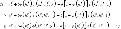
(b) We define the operator
where ut=u(kt−1, ht−1, γt, kt, ht, lt) represents the momentary utility of period t after substituting consumption from budget constraint (7).
To show that T is a contraction, we verify that it satisfies Blackwell's sufficiency conditions.
First, suppose
,
and lt∈[0, 1]. Consider any two functions f and ϕ, defined on
. Assume that f(kt−1, ht−1, γt)[ges ]ϕ(kt−1, ht−1, γt) for all
,
,
. Let (kft, hft, lft) and (kϕt, hϕt, lϕt) attain Tf and Tϕ, respectively, for any
,
,
. After denoting uft=u(kt−1, ht−1, γt, kft, hft, lft) and uϕt=u(kt−1, ht−1, γt, kϕt, hϕt, lϕt), we have
Therefore, T is monotone.
Second, for any positive constant m[ges ]0, we obtain
Therefore, T discounts.
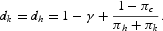
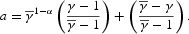
APPENDIX C: CALIBRATION PROCEDURE
We calibrate the parameters of the model in the steady state. We define a steady state as a situation in which all variables of the stationary economy (6)–(8) take constant values. In the steady state, instead of switching between two different growth rates,
and, consequently, two levels of labor productivity,
, the economy faces a constant growth rate, γ, and a constant level of labor productivity, a, given by
By evaluating FOCs (10)–(12) and constraint (7) in the steady state, we obtain, respectively,
where n=1−l. In terms of the ratios πc, πk, and πh, conditions (C.3), (C.4), and (C.6) can be rewritten as
Equations (C.7)–(C.9) provide a basis for calibrating the parameters B, δ, dk, and dh.
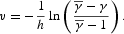
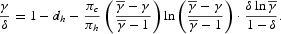
We now calibrate the parameter
. From (C.1) we have that
and, consequently,
The last result allows us to rewrite condition (18) as follows:
By solving this equation numerically, we obtain the value of the parameter
. Next, we restore the technology by using (C.2)
Given the technology level, we compute the capital-to-labor ratio,
and find the steady-state level of output, y=an(k/n)α. Subsequently, we compute the steady-state human capital stock, h=πhy, and calibrate the parameter v by using equa- tion (23).
In sum, our calibration procedure identifies uniquely the model's parameters
so that the model reproduces {πc, πk, πh, n, γ}.
The steady-state expression of the FOCs of Kydland and Prescott's (1982) model coincides with (C.7)–(C.9) under πh=0. For given {πc, πk, n, γ}, these conditions identify the values of B, δ, and dk.
APPENDIX D: SOLUTION PROCEDURE
To solve for equilibrium in the model, we employ a variant of the parameterized expectations algorithm (PEA) by Den Haan and Marcet (1990). A further description of the PEA and its applications can be found in Marcet and Lorenzoni (1999). To ensure the convergence of the PEA, we bound the simulated series on initial iterations as described in Maliar and Maliar (2003b).
Since there are two intertemporal FOCs, we must parameterize two conditional expectations. We parameterize the right-hand side of FOC (11) as follows:15
We find that using a more accurate second-order polynomial approximation for the decision rules instead of the first-order one affects the solution very little but raises the computational expenses significantly.
The second intertemporal FOC may not be parameterized in this manner because there would be two equations identifying consumption and no condition identifying physical and human capital. To deal with this complication, we premultiply both sides of FOC (12) by ht and parameterize the right-hand side of the resulting condition as follows:
We approximate the optimal value function V(kt−1, ht−1, γt) by a second-order polynomial
We use the following iterative procedure:
- Step 1. Fix the initial coefficients {βi}4i=1, {λi}4i=1 and {ηi}10i=1. Fix initial condition (k−1, h−1). Draw a random series of numbers {ut}Tt=0 from a uniform distribution, [0, 1], and fix it.
- Step 2. Given {βi}4i=1 and {λi}4i=1, use (7), (10), (27), and (28) to calculate recursively {cgt+1, cbt+1, lgt+1, lbt+1, kt, ht, γt}Tt=0. To determine a sequence of the economy's states, use the series {ut}Tt=0. Specifically, for each t, compute the probability φ(ht) and compare it with the random number ut. If φ(ht)[ges ]ut, then assume ; otherwise, take γt=1.
- Step 3. Given {ηi}10i=1 and {cgt+1, cbt+1, lgt+1, lbt+1, kt, ht, γt}Tt=0, from the Bellman equation (9), compute the series of values of the value function in the two states, {V(kt−1, ht−1, γt), V(kt−1, ht−1, 1)}Tt=0. Restore the variables in the right-hand sides of FOCs (11) and (12). Run the nonlinear least-square regressions of the corresponding variables on the functional forms (D.1), (D.2), and (D.3). Use the reestimated coefficients {βi}4i=1, {λi}4i=1 and {ηi}10i=1 as input for next iteration.
Iterate on the coefficients {βi}4i=1, {λi}4i=1, and {ηi}10i=1 until a fixed point is found. To solve for a fixed point, we use a built-in MATLAB gradient-descent procedure “f solve.” The length of simulations was T=5,000.
We also apply the PEA for calculating a solution to Kydland and Prescott's (1982) model. We parameterize the intertemporal condition of the stationary version of the model as follows:
We fix initial condition (k−1, θ−1) and the initial coefficients {ei}3i=1. We draw a series of technology shocks, {θt}Tt=1, and fix it. As above, we iterate on the coefficients {ei}3i=1 until we find a fixed point.
We wish to express our sincere gratitude to the editor, an associate editor, and two anonymous referees for many valuable comments and suggestions. All errors are ours. This research was supported by the Instituto Valenciano de Investigaciones Económicas and the Ministerio de Ciencia y Tecnología de España, the Ramón y Cajal program, and BEC 2001-0535.