INTRODUCTION
Most work on explaining international income differences is based on the underlying assumption that countries have distinct long-run growth paths. Sala-i-Martin (1996) claims that the primary reason to concentrate on steady-state analysis is that it is easy to study, and it is therefore a springboard on which to advance richer explanations of economic growth. Support for steady-state analysis is even stronger in the empirical literature [e.g., see Mankiw et al. (1992) (MRW), Nonneman and Vanhoudt (1996), and Dinopoulos and Thompson (2000)], which focuses on estimating reduced-form steady-state specifications that successfully fit the cross-country data.1
MRW explain 78% of income variation across 98 countries. Nonneman and Vanhoudt (1996) extend MRW to include R&D capital and also explain 78% of the income variation across the OECD countries.
Even though the literature has embraced steady-state analysis, it is widely accepted that income disparities are most likely due to some combination of steady-state differences and transition toward the steady state.2
For example, King and Rebelo (1993) emphasize the important role of adjustment paths in explaining growth experiences. Barro and Sala-i-Martin (1995, ch. 11) report estimates of regional σ-convergence within countries that allow for a large role for transition dynamics.
In this paper we provide additional evidence supporting the role of transition dynamics in explaining cross-country income differences. We perform a novel exercise in which we take the opposite viewpoint to steady-state analysis: namely, we assume that all countries approach the same balanced growth path, and that their income levels differ because they are at different points along the transition.
More specifically, we study the transition dynamics predictions of a growth model with endogenous technical progress physical and human capital accumulation, and we evaluate their performance in explaining income disparities across countries. Even though the model in this paper exhibits certain properties that can stand out in their own right, the focus is on taking the transition dynamics predictions of the model to the data by using calibration techniques.
The model considered here is an extended version of Jones' (2002) framework with two modifications: First, we allow for human capital stock to accumulate endogenously over time, and second, technology imitation in our model is costly. Following Bils and Klenow (2000), we include the above two modifications to make the model more appropriate to analyze countries at different levels of development. We choose Jones' nonscale growth model—admittedly only one of various candidates—because it has succeeded in reconciling important properties of the data such as increasing R&D intensity and rising educational attainment levels with constant output growth rates. It is important to mention, however, that the nonscale feature of the model is present only along the balanced-growth path; scale effects are possible along the transition, as recently pointed out, for example, by Dinopoulos and Thompson (1998). The model therefore does not impose nonscale behavior to developing economies that maybe in transition to the steady state. Finally, the nonscale growth model can generate the customary MRW-type steady-state equation, as pointed out by Howitt (2000), a property that will prove helpful in our analysis.
The main finding from this exercise is that transition dynamics are able to explain the cross-country income level dispersion as well as steady-state regressions do. It is also shown that the transition dynamics of the model can explain (in various degrees) other stylized facts on economic development, such as cross-country dispersion of growth rates, cross-country dispersion of saving/investment rates, and cross-country equality of real interest rates. Overall, we interpret our results as suggesting that a world in which nations move along their balanced-growth paths is as likely as a world in which countries move along adjustment paths toward a common (very long run) steady state.
Work related to our approach—using calibration and taking the implications of growth models to the data—includes Christiano (1989), King and Rebelo (1993), and Chari et al. (1997). Implications of the nonscale growth model considered in this paper have been extensively explored by Eicher and Turnovsky (1999a,b, 2001), and Perez-Sebastian (2000). Unlike us, these authors do not consider human capital. Recent work by Jones (2002) questions steady-state analysis; however, he focuses only on the U.S. experience.
The rest of the paper is organized as follows. Section 2 presents the basic model. In that section, we establish the economic environment and examine the steady-state and transition dynamics properties of the model. The numerical analysis is presented in Section 3. In that section, we simulate the adjustment path, assess how well it fits the cross-country output data, and examine how well it explains various development-stylized facts. In Section 4, we perform sensitivity analyses on key parameter values used in the calibration exercise. Section 5 concludes.
MODEL
In this section, we present our model. First, we outline the economic environment under which households and firms operate. Then we solve the socially optimal problem. Our exposition is focused on aggregate technologies. The main reason is that the human-capital technology incorporated in this paper cannot be easily derived from a decentralized setup due to aggregation problems.3
See note 6 for a discussion on the aggregation problem of this approach.
Economic Environment
The economy consists of identical infinitely lived agents, and population grows exogenously at rate n. Agents have preferences only over consumption, and choose to allocate their time endowment in three types of activities: consumption-good production, R&D effort, and human capital attainment.
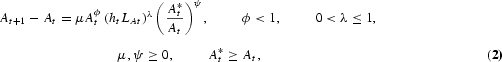
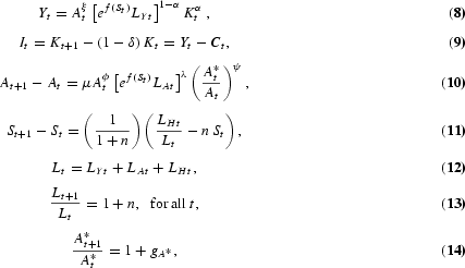
Our model economy is characterized by the following three equations: First, at period t, output (Yt) is produced using labor (LYt) and physical capital (Kt) according to the following aggregate Cobb-Douglas technology:
where ht represents the effectiveness of average human capital level on labor, α is the share of capital, ξ is a technology externality, and At is the economy's technical level.
Second, the R&D equation that determines technological progress is given by
where LAt is the portion of labor employed in the R&D sector at time t, A*t is the worldwide stock of existing technology that grows exogenously at rate
, ϕ is an externality due to the stock of existing technology, and λ captures the existence of decreasing returns to R&D effort. The above R&D equation is the one proposed by Jones (1995, 2002) plus a catch-up term (A*t/At)ψ, where ψ is a technology-gap parameter. The catch-up term is also consistent with the “relative backwardness” hypothesis of Findlay (1978) that the rate of technological progress in a relatively backward country is an increasing function of the gap between its own level of technology and that of the advanced country.
4 Nelson and Phelps (1966) are the first to construct a formal model based on the catch-up term. Parente and Prescott (1994) notice that this formulation implies that development rates increase over time (with A*t), and provide empirical evidence that is consistent with this implication. Benhabib and Spiegel (1994) find evidence in favor of an R&D equation with imitation in a large sample of countries.
Third, we have the schooling equation that determines the way by which human capital accumulates. The human capital technology follows Bils and Klenow (2000), who suggest that the Mincerian specification of human capital is the appropriate way to incorporate years of schooling in the aggregate production function. Following their approach, human capital per capita is given by
where f(St)=ηSβt, η>0, β>0; and St is the labor force average years of schooling at time t. The derivative f′(St) represents the return to schooling estimated in a Mincerian wage regression: an additional year of schooling raises a worker's efficiency by f′(St).
5 For the original discussion on Mincerian wage regressions, see Mincer (1974). For recent discussion of the advantages of the Mincerian approach in growth modeling and estimation, see Bils and Klenow (2000) and Krueger and Lindahl (2001).
,
6 To be fully consistent with the Mincerian interpretation,
, where sit is the educational attainment of worker i at date t. The mapping between this expression and equation (3) is not straightforward, and has not been addressed by the literature, with the exception of Lloyd-Ellis and Roberts (2002) who perform only balanced-growth path analysis in a finitely lived agent framework. The difficulty arises because different cohorts can possess different schooling levels. To make both expressions consistent, we could assume that the first generation of agents pins down the workers' educational attainment, and that posterior cohorts are forced to stay in school until they accumulate this educational level. In this way, all workers would have the same years of education (i.e., sit=St for all i), hence
. However, introducing this into the model would force us to keep track of the different cohorts' years of education across time, thus making the transitional dynamics analysis much more cumbersome, if not impossible. We leave this important issue to future research.
We assume that, each period, agents allocate time to human capital formation only after output production has taken place.
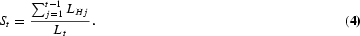
7 The primary reason for the particular timing of events is mathematical tractability. In particular, this timing allows writing the motion equation of St+1 as a function of St and LHt [see equation (5)]. If timing was reversed, we would obtain the state variable St+1 as a function of St and LH,t+1 that could make the optimal control problem significantly more difficult to solve.
Let
LHt be the total amount of labor invested in schooling in the economy at date
t. Assume that at some point in time, say period 1, the average educational attainment equals
zero. Next period, given that consumers live for ever, the average years of schooling will be
S2=
LH1/
L2, where
Lt is the labor size at date
t. In period 3,
S3=(
LH1+
LH2)/
L3, and so on. Hence, the average educational attainment can be written as
From equation (4), we can write
which in turn implies
It is important to notice that the above human capital technology differs from the one employed in Jones (2002). In particular, Jones assumes that education investment fully depreciates each period or, in other words, that human capital does not accumulate. However, the optimal allocation to investment in education declines along the adjustment path and therefore without human capital accumulation, human capital index is larger in lower-income nations; clearly a counterfactual result. Our equation (6) does not suffer from this counterfactual result because the value of S rises with the income level, as the international evidence suggests.
Social Planner's Problem
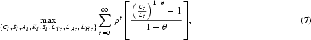
Let Ct be the amount of aggregate consumption at date t. A central planner would choose the sequences {Ct, St, At, Kt, LYt, LAt, LHt}∞t=0 so as to maximize the lifetime utility of the representative consumer subject to the feasibility constraints of the economy, and the initial values L0, K0, S0, and A0. The problem is stated as follows:
subject to
where θ is the inverse of the intertemporal elasticity of substitution, ρ is the discount factor, and δ is the depreciation rate of physical capital. Equation (9) is a feasibility constraint as well as the law of motion of the stock of physical capital; it states that, at the aggregate level, domestic output must equal consumption plus physical capital investment, It. Equation (12) is the labor constraint; the labor force—that is, the number of people employed in the output and the R&D sectors—plus the number of people in school must be equal to population.
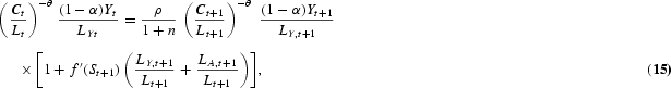
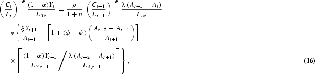
Solving this dynamic optimization problem obtains the Euler equations that characterize the optimal allocation of labor in human capital investment, in R&D investment, and in consumption/physical capital investment, respectively, as follows:
At the optimum, the planner must be indifferent between investing one additional unit of labor in schooling, R&D, and final output production. The LHS of equations (15) and (16) represent the return from allocating one additional unit of labor to output production. The RHS of equation (15) is the discounted marginal return to schooling, taking into account labor growth. The RHS term in brackets arises because human capital determines the effectiveness of labor employed in output production as well as in R&D. The RHS of equation (16) is the return to R&D investment. An additional unit of R&D labor generates [λ(At+1−At)]/LAt new ideas for new types of producer durables. Every new design increases next period's output by ξYt+1/At+1 and R&D production by dAt+2/dAt+1 times [(1−α)Yt+1]/LY,t+1{[λ(At+2−At+1)]/LA,t+1}−1, where the term [(1−α)Yt+1]/LY,t+1{[λ(At+2−At+1)]/LA,t+1}−1 gives the value of one additional design that equalizes labor wages across sectors. Euler equation (17) is standard and states that the planner is indifferent between consuming one additional unit of output today and converting it into capital (thus consuming the proceeds tomorrow).
Steady-State Growth
We now derive the model's balanced-growth path. Solving for the interior solution, equation (12) implies that in order for the labor allocations to grow at constant rates, LHt, LYt, and LAt must all increase at the same rate as Lt. This means that the ratio LHt/Lt is invariant along the balanced-growth path. Hence, equation (11) implies that, at steady state (SS),
is constant and is given by
where
. Equation (18) shows that along the balanced-growth path the economy invests in human capital just to provide new generations with the steady-state level of schooling.
Let lowercase letters denote per capita variables, and gx=Gx−1 denote the growth rate of x. The aggregate production function, given by equation (8), combined with the steady-state condition gY,ss=gK,ss delivers the gross growth rate of output as a function of the gross growth rate of technology as
Since GA,ss is a constant, it follows from equation (2) that
Equation (20) shows the relationship between the technology frontier growth rate and the technology growth rate of the model economy. Since
, it is easy to show that there is a unique point at which
Given the nature of the experiments that we want to carry out, we focus on the special case in which all countries grow at the same rate in steady state. That is, we assume that
is given by expression (21), and therefore so is GA,ss.
8 Alternatively, we could assume that the technology leader shifts the world technological frontier outward according to equation (2), which now reduces to
where A*t/At=1 as imitation is not possible at the frontier; and * denotes the value that variables take in the leading country. In such case
as in Jones (1995, 2002). Assuming that n=n*, and substituting G*A into equation (20) delivers equation (21).
This in turn implies that
Consistent with Jones (1995, 2002) our balanced-growth path is free of scale effects. The reason why our model's long-run growth is equivalent to that of Jones even in the presence of a schooling sector, is that at steady state the mean years of education, St, reaches a constant level
.
Transition Dynamics
The aggregate production function, equation (8), suggests that we normalize variables by the term
. We then rewrite consumption, physical capital, and output as
,
, and
), respectively. Using equation (15) gives
where uYt and uAt are the labor shares in R&D and final-output production at time t, respectively. From the R&D equation (2), we get
where T=A*t/At; and υ=μ(A*t)ϕ−1Lλt, which is a constant.
9 To show that υ is constant requires some algebra. Rewriting the equality in its gross growth form,
, and given that
, it follows that υt+1/υt=1. Notice that had A*t not grown according to equation (21), υ could not be constant, making the simulation exercise much more difficult to implement.
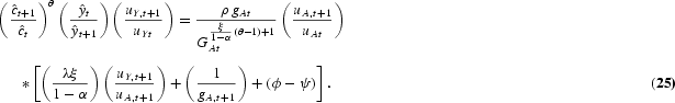
From equation (16) we get
Finally, from equation (17) we get
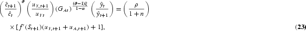
The system that determines the dynamic equilibrium normalized allocations is formed by the conditions associated with three control and three state variables as follows:
Control Variables:
- Euler equation for labor share in schooling, uHt: Equation (23)
- Euler equation for labor share in R&D, uAt: Equation (25)
- Euler equation for consumption, : Equation (26)
Subject to the constraint uYt=1−uAt−uHt.
State Variables:
- Law of motion of human capital, St: Equation (6)
- Law of motion of technology, At: Equation (24)
- Law of motion of physical capital
where
and
NUMERICAL ANALYSIS
In this section we take the proposed model to the data by means of a calibration exercise. We first assign values to the parameters. Then, we simulate the transition dynamics, and compare their predictions to the data. Because there is no analytical solution to our system of Euler and motion equations presented in the preceding section, we resort to numerical approximation techniques. More specifically, we follow Judd (1992) to solve the dynamic equation system, approximating the policy functions by employing high-degree polynomials in the state variables.10
In particular, the parameters of the approximated decision rules are chosen to (approximately) satisfy the Euler equations over a number of points in the state space, using a nonlinear equation solver. A Chebyshev polynomial basis is used to construct the policy functions, and the zeros of the basis form the points at which the system is solved; that is, we use the method of orthogonal collocation to choose these points. Finally, tensor products of the state variables are employed in the polynomial representations. This method has proven to be highly efficient in similar contexts. For example, in the one-sector growth model, Judd (1992) finds that the approximated values of the control variables disagree with the values delivered by the true policy functions by no more than one part in 10,000. All programs were written in GAUSS and are available by the authors upon request.
Calibration
Because relative values of the cross-country data to which we compare the predictions of the model are taken with respect to U.S. levels, we calibrate the model parameters using, when possible, U.S. data as the steady-state outcome. Table 1 presents the parameter values used to carry out the simulations. We choose a value of 0.06 for the depreciation rate (δ), a value of 0.96 for the discount factor (ρ), and 0.36 for the capital share of output (α), which are standard in the literature. To assign values to per capita income growth rate in steady state (gy,ss), and to population growth rate (n), we follow Jones (2002). In particular, we set gy,ss equal to 2%, the average growth of output per hour worked between 1950 and 1993 in the United States, and n equal to 1.2%, the average growth rate of the labor force in the G-5 countries (France, West Germany, Japan, the United Kingdom, and the United States) during the period 1950–1993. The reason for using the average growth rate of labor in the G-5 rather than any other group of countries (or, for that matter, the whole sample) is that the main role of population growth rate in the model is to move the world technology frontier in steady state, and clearly the majority of world research effort is conducted in the G5 countries.11
Coe et al. (1997) report that in 1990, industrial countries accounted for 96% of the world's R&D expenditure.
Regarding the value of the elasticity of output with respect to the technology, Griliches (
1988) reports estimates of ξ between 0.06 and 0.1. We choose to follow Eicher and Turnovsky (
1999b,
2001) and set ξ=0.1.
It is not clear what the steady-state value of the average educational attainment ought to be, given that mean years of schooling has been increasing over the past decades in most developed countries. We choose to set
to 12.5, to match the 1993 U.S. figure reported by Jones (2002). From equations (18), (23), and (26), it can be easily shown that the values of
, n, and Gy,ss imply an interest rate [given by the RHS of (26)] at steady state of 7.9%, which is well within U.S. observations.
12 For example, King and Rebelo (1993) report average real rates of return for the period 1926–1987 on different U.S. securities that vary between 0.42% and 8.80%.
In turn, substituting the values of the steady-state interest rate, ρ,
n, and
Gy,ss into equation (15) implies that the inverse of the intertemporal elasticity of substitution (θ) is 1.19, which is well within the empirical estimates.
13 Estimates of θ by Hall (1988) and Attanasio and Weber (1993) range from 1 to 3.5. For a recent discussion on estimates of θ, see Guvenen (2002).
Following Bils and Klenow (
2000), we use Psacharopoulos' (1994) cross-country sample on average educational attainment and Mincerian coefficients to estimate η and β. Given
f(
S)=η
Sβ, we can construct the regression
where Minceri=f′(Si) is the estimated Mincerian coefficient for country i; a and b equal ln(ηβ) and (β−1), respectively; and εi is a disturbance term. We obtain η=0.69 and β=0.43, which are very close to estimates by Bills and Klenow (2000).
Finally, we calibrate the R&D technology parameters. As a benchmark case, we set λ=0.5, and using equation (21) we recover the value of ϕ= 0.95.14
In the next section, we perform a sensitivity analysis on key parameters of the model.
Given that the effect of the parameter ψ is purely transitional, we follow Parente and Prescott (
1994) and calibrate it to replicate miraculous experiences.
15 As in Parente and Prescott (1994), we smooth the data series involved in the calibration of ψ using the Hodrick-Prescott filter with the smoothing parameter equal to 25.
In particular, we choose ψ so as to reproduce the relative output per worker path between 1960 and 1990 in Japan and between 1963 and 1990 in South Korea.
16 South Korea's rapid convergence toward U.S. income levels began around 1963. Japanese convergence, on the other hand, started right after WWII. Unfortunately, the Japanese Education Department does not possess estimates of the average educational attainment before 1960. We are grateful to Tomoya Sakagami who has attempted to obtain these data for us.
We choose to calibrate ψ for these two economies because they have experienced distinctly different development experiences, notwithstanding their equally impressive growth rates (Japan grew at 5.2% per year and South Korea at 6.5% per year during the relevant periods), therefore making it possible to obtain values for ψ that are potentially quite different. The South Korean development experience implies a value for ψ of 0.18, whereas the Japanese development experience implies that ψ equals 0.22. The initial values of the stock variables and the output data used to calibrate ψ, as well as the accuracy measures, are presented in
Table 2.
Transition Dynamics Predictions
Unlike steady-state regressions, in this section we assume that all countries belong to the same transitional path, approaching a unique, common balanced-growth path. Specifically, we perform two experiments as follows: First, we simulate the dynamics of a representative economy and study how well its adjustment path represents the cross-country data on key variables such as the state variables, interest rates, investment rates, and output growth rates. Second, we propose an exercise similar in spirit to that of MRW, which tries to assess how much of the cross-country output variation can be explained by transition dynamics.17
In addition, we have investigated the asymptotic speed of convergence implied by the model—the rate by which a country's output converges to its balanced growth path once the country is sufficiently close to its long-run equilibrium. In our model, this speed is given by the largest eigenvalue among those contained in the unit circle. Parameter values in the neighborhood of those employed in our calibration deliver speeds of convergence that vary between 1.06%–2.08%, consistent with most empirical evidence. Our results are consistent with the finding of Eicher and Turnovsky (1999b, 2001), that moving from one-sector to multisector nonscale growth models with endogenous technological change leads to severe reduction in the asymptotic speed of convergence, and allows convergence speeds to vary across time and variables.
The primary motivation for these two experiments is to examine how well the transitional dynamics of the proposed model can explain cross-county per capita income dispersion and other important stylized facts.
To carry out the first experiment, we need to estimate the policy rules that take state variables from given initial values to the steady state. Doing so requires the following two conditions: (a) given that the further away we move from the balanced-growth path, the lower the accuracy degree of the numerical approximation, we choose the initial values so that the numerical approximation provides a maximum-error measure of about 2% (see Table 2); (b) we start the adjustment paths inside the cloud of cross-country observations that compose our comprehensive sample.18
Our comprehensive sample (79 countries) consists of the MRW's non-oil nations for which average years of schooling per worker are available from the STARS (World Bank) database, minus Ireland, which is eliminated from the sample due to implausibly high schooling figures. For further discussion on the data, see the data appendix.
Given conditions (a) and (b), we pick an initial value for the relative physical capital stock per worker of 5.4%, an initial value for the average educational attainment of 2.7 years, and an initial value for relative total factor productivity (TFP) of 55.2% so as to generate a relative GDP per worker level of 10.4.
19 Notice that, for relative GDP per worker level of 10.4, our numerical approximation commits a maximum error of 2.38% in accordance with condition (a); see Table 2.
,
20 In our simulation exercise, TFP is broadly defined and includes everything not already captured by the other two stock variables, S and K.
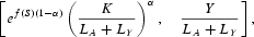
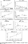
The goal of the first experiment is to see how well the transition dynamics of the model can explain important stylized facts such as cross-country dispersion of growth rates, cross-country dispersion of saving/investment rates, and cross-country equality of real interest rates. Figure 1 depicts cross-sectional data, along with off-steady-state predictions for physical capital, average years of schooling, TFP, interest rates, investment rates, and relative output growth. It is evident that the plotted data show wide cross-country dispersion in all variables, except for real interest rates, which are quite uniform across nations above the 25th percentile. State variables (K, S, A) generally increase with the relative level of output, and investment and growth rates generally depict weak inverted-U shapes, starting low and achieving their maximum values for middle-income nations.21
Following Jones (1997), we compute real interest rates (return to capital) as the marginal product of capital, that is, αY/K. As Jones does, we find that the resulting returns for countries below the 25th percentile are highly heteroskedastic, and that some nations present returns above 100%. The main pattern that we observe, however, is a large amount of uniformity in the returns to capital above the 25th percentile.
Adjustment paths for the non-oil sample: Benchmark case. Note: RGDPW is relative GDP per worker.
With fixed initial and final values of the state variables, the question is how well the transition path follows the data cloud in between. If we look at the charts in panels A, C, and E of Figure 1, the primary finding is that the simulated dynamics seem to fit well across the state-variable observations. These charts illustrate a number of other points worth noting. First, notice that a larger degree of relative backwardness (i.e., a larger value of ψ) induces faster technology catch-up, and slower human capital accumulation, making the adjustment paths better fit the data. Second, the simulated physical and human capital levels tend to diverge with respect to the rich countries' data. This is the result of calibrating the steady state to U.S. data. The two variables' divergent processes, however, offset each other and, as a result, the technology path captures well the observations.
Finally, let us pay attention to the charts in Panels B, D, and F of Figure 1. Below the 30th percentile in panel F, output-growth predictions are too large; thus, our model overpredicts output growth at early stages of development. Above the 30th percentile, however, predictions fall across the cloud of observations; thus, our model does much better in predicting output growth at later stages of development. In addition, panels B and D show that predictions capture the uniformity of the real interest rates (return to capital) above the 25th percentile, and are consistent with investment rates above the 35th percentile. As is the case with output growth, our model is weaker in replicating interest and investment rates at early development.
Our first experiment has shown that transition dynamics capture fairly well the cross-country equality of the real interest rates, and generate investment rates that are plausible, even though lower investment ratios at early levels of development would better capture the dispersion of the data. The main explanation for this lower dispersion of the predictions is probably a larger degree of market imperfections and distortions in less developed countries, something that the model cannot explain, and that can be perceived as a source of differences in steady states or in convergence speeds along the transition. The predicted output growth rates, on the other hand, are clearly impossible for countries with relative real GDP below the 30th, but reasonable for more developed nations. For the sake of comparability between transition dynamics predictions and steady-state regression predictions, it is important to mention that steady-state predictions are not very successful in accounting for the observed cross-country income growth dispersion either. Steady-state growth regressions of the MRW type need to make use of transitional factors to be able to minimally fit the data.
Can Transition Dynamics Explain the Cross-Country Output Data?
We now turn attention to the main issue of the paper: How well can the transition dynamics of the model explain cross-country income dispersion? More specifically, our second experiment tries to assess quantitatively how well the transition dynamics fit the output-per-worker data. This is important because fitting the cross-country income data is where steady-state regressions achieve their great success and therefore such an experiment is well motivated. Since we want to compare the transition dynamics predictions of our model with those of steady-state income regressions, we need to construct a measure of fit for transition dynamics that can be compared with a measure of fit in level regressions (namely, the OLS R2).
Taking logs in the Cobb-Douglas representation of the aggregate production function, and substituting inputs for their balanced-growth values, we end up with a standard in the literature steady-state econometric equation
where
is the estimate of output per worker;
and
represent estimates of k and S, respectively, derived from steady-state conditions using investment rates;
are estimated coefficients; and ε is a random disturbance term. Evidently, for the underlying model to be consistent with the data, estimated coefficients must be plausible according to the weight assigned by the national accounts to the different inputs. To each combined{\pagebreak} value
the regression assigns a predicted output level in log-scale, and all of the predicted output levels are in turn translated into a measure of fit (the OLS R2).
Following an equivalent procedure, we first calculate for each country the combined value ef(S)(1−α)[K/(LA+LY)]α implied by the data, imposing the calibrated parameter values. Notice that this extendedstate variable represents the per worker human capital term (i.e., ef(S)(1−α)), and the per worker physical capital term {i.e., [K/(LA+LY)]α}, as specified in the production function given by equation (8). Second, to each country's value of the combined state variable, we assign the output per worker level Y/(LA+LY) predicted by the transition path.22
Because the simulated adjustment path is a discrete set of pairs
we use interpolation methods to generate the predicted output level.
As mentioned previously, to generate the adjustment-path simulation, we employ initial values for the relative per worker physical capital stock, and the average educational attainment of 5.4% and 2.7 years, respectively. It works out that these two initial values imply a minimum value of the relative extended state variable of 18.9%. The sample that we employ to compute the measure of fit must then consist of those 51 nations that provide values of the extended state variable above 18.9%.23
An asterisk identifies these 51 nations in the data table contained in the Appendix.
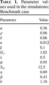
Figure 2 displays the actual output data (plot), and the predicted output data for the two values of ψ (continuous lines). To assess the fit of the adjustment paths, we employ the following statistic, which is equivalent to the OLS R2:
where
and xj are the predicted and actual values of variable x for country j, respectively; and N is the number of countries included in the sample. Our variable x must be the natural log of relative GDP per worker to make the pseudo-R2 comparable to the R2 reported in steady-state regressions.
Adjustment-path predictions of GDP per worker for 51-nation sample: Benchmark case. Note: GDPW and KW denote GDP per worker and physical capital per worker, respectively.
For the adjustment-path predictions expressed in natural logs, Table 3 reports estimates of the pseudo-R2. As it is shown, the transition path can explain up to 76% of the variation of relative output per worker in both the 51 non-oil and the 21 OECD samples. These numbers compare pretty well with the R2 obtained by steady-state regressions. For example, MRW report a maximum R2 of 78 for their non-oil sample, and 28% for the OECD group. Nonneman and Vanhoudt (1996), in turn, obtain an R2 of 78% for OECD nations. These numbers are just a bit above the ones delivered by the transition predictions.
How can one interpret our results in the context of the existing empirical literature? Our results imply that the transition dynamics of an R&D model with endogenous human capital can explain the cross-country output variation as well as the more popular steady-state regressions can. Our findings do not discredit in any way the common steady-state regression exercises. They do, however, provide evidence that transition dynamics may be at least as important as steady states in explaining income differences.
ROBUSTNESS ANALYSIS OF THE RESULTS
In this section, we perform a sensitivity analysis of our results to changes in key parameter values. In particular, we focus on the R&D technology parameters, the population growth rate, the discount factor, and the elasticity of final output with respect to technology. We mainly study how changes in these parameters affect our measure of fit (Pseudo-R2) that assesses the capacity of the model to explain the cross-country dispersion of output per worker.
It is known from Jones (1995) and Eicher and Turnovsky (1999b, 2001) that the type of nonscale R&D growth models that we use is highly sensitive to the returns to scale and the shares of technology and labor in the R&D sector. To study the robustness of our results, we carry out sensitivity analyses for different values of the parameters λ, ϕ, and ψ.
Estimates of the labor share in the R&D sector, λ, found in the literature vary from 0.2 [Kortum (1993)] to 0.75 [Jones and Williams (2000)]. We start the robustness analysis by examining how the measure of fit changes when we replace our baseline value of λ=0.5 with the more extreme values λ=0.25, 0.75. As shown in the first row of results in Table 4, when we reduce λ from 0.5 to 0.25, the adjustment path generates a pseudo-R2 up to 72% for the 51-country sample and up to 63% for the 21-OECD-country sample. As expected the decrease in λ results in lower steady-state per worker income growth rates (gy,ss falls from 2% to 1%). However, the effect of lowering λ on the measure of fit comes mainly from the increase in the steady-state educational attainment level,
, which goes from 12.5 up to 13.1 years, and moves the predictions of S away from the cloud of points.24
The inverse relationship between λ and
is the result of labor reallocation between the schooling sector and the R&D sector. For example, a decline in λ decreases the return to working in the R&D sector, therefore making the R&D activity relatively less attractive than schooling. This triggers labor movement from the R&D sector to the schooling sector, and then
increases.
The second row of
Table 4 confirms this point. In particular, we show that when we modify θ to obtain the baseline value
, the measure of fit increases up to 76% for the 51-country sample and 73\for the 21-OECD-country sample. When, on the other hand, the parameter λ is 0.75 (see third row of results in Table 4), then the pseudo-R2 rises to 77% and 79% for the 51-country and 21-OECD-country samples, respectively. The forth row of results in the table (in which we modify θ to obtain the baseline value
), once again confirms that the induced variation in the steady-state average educational level is the main cause of the change in the measure of fit. In short, the underlying intuition for the increase in the pseudo-R2 as the parameter λ rises is the same as that explaining the benchmark case: A lower rate of human capital formation coupled with a faster technological catch-up process make the predictions better fit the data in Figure 1.
The empirical literature does not offer much guidance in choosing a reasonable value for technology externality ϕ. In our benchmark case, the value for this parameter (ϕ=0.95) is pinned down by the balanced-growth equation (22). Some authors, such as Eicher and Turnovsky (1999b, 2001), however, argue that a value of ϕ=0.95 may be too large. The fifth and sixth rows of results in Table 4 show that lower values of ϕ actually improve the fit of the predicted dynamics. For example, the pseudo-R2 takes on values up to 80% for both country samples considered when ϕ=0.70 and we maintain
. The pseudo-R2 increases to 82% for the 21-OECD-country sample when ϕ declines further to 0.50.25
In this exercise, we modify the value of θ to maintain
. As before, if instead the parameter θ remains equal to 1.19, then the fit becomes worse because
rises. However, when θ=1.19, and ϕ=0.50, the pseudo-R2 is larger than the numbers in the first row of Table 4, and to save space we have omitted this case.
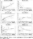
To understand the forces that drive the increase in the pseudo-R2 when ϕ declines, let us focus on Figure 3, which presents the adjustment-path predictions in the case where we assume a low value of ϕ=0.50. Compared to Figures 1 and 2, the improvement is evident in all the panels. The smaller value of ϕ in the R&D equation reduces the total productivity of R&D effort for any given level of A, thus lowering the economy's capacity to grow, as shown in panel F.26
Notice that when ϕ=0.50, gy,ss decreases to 0.19%, a value that might not be impossible in light of new findings by Jones (2002). He argues that the long-run income growth rate for the United States can be considerably smaller than the average value experienced during the past century. Compared to our benchmark, another implication of such decline in growth rates is that the half-life of the convergence process doubles, going from 41 up to 82 years.
At the same time, however, equation (24) and the definition of
v that follows imply that a reduction of ϕ is equivalent to a relatively bigger advantage of technological backwardness. The result is that, compared to the benchmark case, output growth at early stages of development is achieved, devoting more labor to the R&D sector and less to schooling. This, in turn, generates a relatively larger accumulation of technology (panel E) and smaller human capital formation (panel C). The better fit of the average educational attainment and TFP predictions explain the improvement in the pseudo-
R2 delivered by the predicted income levels (see panel G). Finally, the lower elasticity of substitution between present and future consumption (a larger value of θ) is responsible for the lower investment rates and the improved fit shown in panel (D).
27 Adjustment paths similar to those in Figure 3 were produced for all parameter values of λ, ϕ, ψ, n, ρ, and ξ considered in Tables 4 and 5. Since they do not add anything significant to the analysis, they are omitted but are available from the authors upon request.
Adjustment paths for the non-oil sample: ϕ=0.50 case. Note: RGDPW is relative GDP per worker.
We now examine how sensitive the measure of fit is to variations in the catch-up term ψ. We know from our previous results that the pseudo-R2 rises with ψ; the question now is by how much it can vary. Once again we have no guidance about reasonable values of ψ. We decide to try values of 0.1 and 0.3 so that the calibrated values of ψ for Japan and South Korea (0.18 and 0.22, respectively) are within our chosen range. The last row of Table 4 reports our findings. In particular, for ψ=0.1 the pseudo-R2 is 66% for the 51-country sample and 52% for the 21-OECD-country sample, and for ψ=0.3 pseudo-R2 increases to 79% and 80%, respectively. Therefore, the decrease in the pseudo-R2 can be substantial for low values of ψ.
Table 5 provides the measure of fit for changes in other important parameters: the population growth rate (n), the discounting coefficient (ρ), and the elasticity of final output with respect to technology (ξ). Because the pseudo-R2 is always larger for ψ=0.22, the table presents results only for the ψ=0.18 case. An alternative value of n is given by its average growth rate in the sample. As we include more developing nations, the average population growth rate increases. For instance, the average n for the 51-country sample equals 2%. Compared to the numbers in the first column of Table 3, the first row of Table 5 shows that if we set n=0.02, the pseudo-R2 goes up to 80% and 76%. The reason is the decline in
that equals 9.0 in the new scenario. If we modify θ to obtain the baseline value
(then θ=0.66), the measure of fit decreases to 68% and 61%. This occurs for two reasons: the higher growth rate of output per worker caused by the increase in n, and the larger elasticity of intertemporal substitution (1/θ). The primary effect of these two changes in our experiments is always a faster human capital formation, which, as we know, is bad for the fit.
We next move the value of ξ. When we try the lower bound reported by Griliches (1988) (i.e., ξ=0.06), the pseudo-R2 increases (third and fourth rows of results in Table 5). Now, the lower value of the elasticity of final output with respect to technology requires a larger initial technology gap to generate the same relative TFP [given by Aξ in equation (1)]. This larger initial technology gap, in turn, increases the initial productivity of R&D, and R&D investment rises at the expense of schooling. The consequence is relatively faster TFP growth and slower human capital formation, which is good for the fit.
Finally, the effect of changes in the value assigned to ρ are presented in rows 5 to 8 in Table 5. The fifth row suggests that if the discounting parameter rises to 0.97, future production capacity becomes more valuable for agents, and the steady-state average educational attainment increases to 16.4 years. This clearly moves the predicted evolution of S away from the cloud of points, producing a much lower pseudo-R2 for output per worker that equals 50% for the 51-country sample and 11% for the 21-OECD group. The next row shows that when we fix
, the fit actually improves. In particular, the pseudo-R2 rises to 77% and 76%, respectively. The reason now is the value of θ=1.71, which makes present and future consumption more complementary, and therefore human and physical capital accumulation proceed more slowly. The smoother path of schooling years is responsible for the better fit. Exactly the opposite reason explains why the pseudo-R2 declines to 65% and 53% when we set ρ=0.95 and fix
(last row in Table 5): It requires increasing the degree of substitutability between present and future consumption so that θ=0.66. However, in the seventh row of the table, we see that if we do not fix
, ρ=0.95 makes
decline to 9.8 years and, as a consequence, the fit improves with respect to the benchmark case.
To summarize, the sensitivity analyses on key parameters reveal that for sensible parameter values the predicted income levels explain no less than 72% and 67% of the observed log-income variability across our 51-country sample and 21-OECD-country sample, respectively. Values of λ above 0.5 (and values of ξ below 0.1) take these percentages up to 77% and 79%, respectively. In addition, the measure of fit increases above 80% if we reduce ϕ below 0.7. On the other hand, the fit can decrease below 67% if we allow the steady-state average educational attainment,
, to be above 12.5 years or θ to be lower than 1. However, this seems to us unreasonable because the maximum value of the average years of education in our samples corresponds to the United States and equals 11.35, and because values of θ below 1 go against the available empirical evidence.28
In the Barro and Lee (2001) dataset, the maximum number of years of schooling corresponds to the United States, whose labor force in 2000 had, on average, 12.05 years of formal education. Regarding empirical estimates of θ, see note 13.
The pseudo-
R2 can also decrease below 67% if we let the catch-up term, ψ, take on values below 0.18; however, we do not know if values that low are reasonable. We conclude that our results are quite robust to sensible changes in the shares of labor and technology in the R&D sector, and in other important parameters.
CONCLUSION
In this paper we have studied the capacity of transition dynamics to explain income disparities across nations. In particular, we have taken the dynamic predictions of a nonscale R&D model with endogenous human capital to the data by considering two experiments. First, we have simulated the dynamics of a representative economy and studied the adjustment paths of key economic variables. Second, we have assessed quantitatively how well the transition dynamics fit the output per worker data by proposing a similar in spirit exercise to that of MRW.
Our key finding is that transition dynamics are as successful in fitting the cross-country output per worker data as steady-state regressions. How can we reconcile this finding with the evidence against absolute convergence and in favor of conditional convergence? Standard convergence tests, such as that of Barro and Sala-i-Martin (1995), implicitly assume that the half-life of convergence is the same among countries. Hence, one possibility that can reconcile our finding with absolute convergence is that the time required to complete a given portion of the adjustment path varies across economies. From this viewpoint, the diffusion of ideas ultimately will ensure convergence among nations, and country-specific fundamentals such as institutions, geography, and climate would determine not the steady-state outcome but the half-life of the convergence process. Whether this is the case is an empirical issue that we believe deserves further research.
In addition, we have shown that dynamic predictions of the model can explain (in various degrees) important stylized facts on economic development. In particular, transitional dynamics capture fairly well the cross-country equality of the real interest rates, and generate investment rates that are plausible, especially when the share of technology in R&D is not high. Transition dynamics are less successful in explaining the cross-country dispersion of output growth rates: The predicted rates are impossibly high for the less-developed countries, but reasonable for more developed nations. However, as we explained, this failure is also a feature of steady-state regressions.
The main implication of our results for the empirical growth literature is that by focusing our attention only on reduced-form, balanced-growth predictions we maybe disregarding a substantial part of the story about economic growth. The potential payoff of finding ways to better integrate steady state and transition dynamics conditions can be large, especially in level regression analysis. Indeed, some researchers, for example, Jones (2002), have already begun to venture along this path. Our work also suggests that transition dynamics analysis must play a more extensive role in discriminating among growth theories, especially in light of the recent improvements achieved on numerical algorithms.