
Introduction
Population genetic studies of lichens that compare fungal and algal patterns are particularly interesting because they may tell us how intimately the partners of the symbiosis are tied together and whether their genetic structures are truly coupled, or whether they become uncoupled during the life history of one partner (Piercey-Normore Reference Piercey-Normore2006; Yahr et al. Reference Yahr, Vilgalys and DePriest2006; Werth Reference Werth2010; Werth & Sork Reference Werth and Sork2010; Wornik & Grube Reference Wornik and Grube2010).
Population genetic analyses, and in particular those that compare the patterns of genetic variation among symbionts, or across populations of a single species require a sampling effort assuring that a representative part of the genetic variability has been included. Here, I refer to the individuals sampled within a single site, for example a group of trees or rocks, within a landscape, as a ‘population’. Often, researchers make implicit assumptions about sample sizes (Dixon Reference Dixon2006), but these are rarely stated, let alone tested (but see Zoller et al. Reference Zoller, Lutzoni and Scheidegger1999; Printzen et al. Reference Printzen, Ekman and Tønsberg2003; Lindblom Reference Lindblom2009). One factor calling for large sample sizes is the haploid nature of most lichen-forming fungi, implying that only one gene copy is sampled per individual, as opposed to two gene copies in diploid species. Population genetic statistics depend on the number of gene copies, and thus, haploid organisms would theoretically require a sampling scheme twice as intensive as that of diploid organisms. However, sample sizes are in practice limited by time, budget and other constraining factors, and it may for these reasons not be desirable to employ larger sample sizes than strictly necessary.
Sample sizes vary considerably among the existing population genetic studies of lichen-forming fungi, for instance with respect to the number of populations investigated: 4 (Werth & Sork Reference Werth and Sork2008), 5 (Lättman et al. Reference Lättman, Lindblom, Mattsson, Milberg, Skage and Ekman2009), 7 (Lindblom & Ekman Reference Lindblom and Ekman2006, Reference Lindblom and Ekman2007), 12 (Walser et al. Reference Walser, Holderegger, Gugerli, Hoebee and Scheidegger2005), 12 and 27 (two species investigated, Wornik & Grube Reference Wornik and Grube2010), or 41 (Werth et al. Reference Werth, Wagner, Holderegger, Kalwij and Scheidegger2006, Reference Werth, Gugerli, Holderegger, Wagner, Csencsics and Scheidegger2007); or the total sample size: 72 (Werth & Sork Reference Werth and Sork2008, Reference Werth and Sork2010), 85 (Lättman et al. Reference Lättman, Lindblom, Mattsson, Milberg, Skage and Ekman2009), 225 (Lindblom & Ekman Reference Lindblom and Ekman2006), 230 (Lindblom & Ekman Reference Lindblom and Ekman2007), 290 (Piercey-Normore Reference Piercey-Normore2006), 539 (Wornik & Grube Reference Wornik and Grube2010), 565 (Walser et al. Reference Walser, Holderegger, Gugerli, Hoebee and Scheidegger2005), or 889 (Werth et al. Reference Werth, Wagner, Holderegger, Kalwij and Scheidegger2006, Reference Werth, Gugerli, Holderegger, Wagner, Csencsics and Scheidegger2007). Moreover, there are also major differences in the number of samples analysed per population: 7–15 (Wornik & Grube Reference Wornik and Grube2010), 15–18 (Lättman et al. Reference Lättman, Lindblom, Mattsson, Milberg, Skage and Ekman2009), 18 (Werth & Sork Reference Werth and Sork2008), 25–33 (Lindblom & Ekman Reference Lindblom and Ekman2006), 31–34 (Lindblom & Ekman Reference Lindblom and Ekman2007), 3–41 (Werth et al. Reference Werth, Wagner, Holderegger, Kalwij and Scheidegger2006, Reference Werth, Gugerli, Holderegger, Wagner, Csencsics and Scheidegger2007), and 32–52 (Walser et al. Reference Walser, Holderegger, Gugerli, Hoebee and Scheidegger2005).
A recent study by Lindblom (Reference Lindblom2009) investigated the haplotype diversity and sample sizes in the lichen-forming fungus Xanthoria parietina (L.) Th. Fr. using rarefaction methods, and found that a sample of about 30 thalli per population included a substantial part of the genetic variability at the population level. Open questions are whether this suggested number is 1) similar for taxonomically distant lichen-forming fungi, 2) similar for marker types other than DNA sequences, and 3) high enough to characterize the genetic variability of photobiont populations, or if photobiont populations require a different sampling strategy.
Rarefaction analyses may shed light on these questions. They allow one to infer the smallest sample size at which the slope of the rarefaction curve showing a cumulative diversity measure (e.g., the number of alleles) reaches zero. Once the asymptote has been reached, increasing sample sizes is unlikely to add new alleles. Rarefaction has previously been employed in population genetic studies of lichen-forming fungi to investigate the completeness of haplotype sampling in Cavernularia hultenii Degel. (Printzen et al. Reference Printzen, Ekman and Tønsberg2003), Lobaria pulmonaria (L.) Hoffm. (Zoller et al. Reference Zoller, Lutzoni and Scheidegger1999) and X. parietina (Lindblom Reference Lindblom2009).
Here, rarefaction analyses are performed to evaluate the number of samples required to characterize the allelic diversity in populations of lichen-forming fungi and their photobionts, taking advantage of an existing data set for the epiphytic lichen Lobaria pulmonaria (Werth et al. Reference Werth, Wagner, Holderegger, Kalwij and Scheidegger2006, Reference Werth, Gugerli, Holderegger, Wagner, Csencsics and Scheidegger2007) and its photobiont, Dictyochloropsis reticulata (Tschermak-Woess) Tschermak-Woess. Rarefaction analysis is used to determine whether the required sample sizes differ for fungal and algal populations, both with respect to the number of samples within populations and within a landscape, and for the number of populations. Moreover, I discuss and recommend sample sizes for future population-level studies of lichen-forming fungi and their photobionts.
The questions that I explore are:
1) How many individuals should optimally be sampled per population? Is the number of individuals different for mycobiont and photobiont populations? How many individuals in total should be sampled so that genetic diversity is accurately represented at the landscape scale?
2) How many populations should be investigated in population genetic studies of lichen-forming fungi and their photobionts?
Materials and Methods
Data set
The data has previously been published and has been described in detail by Werth et al. (Reference Werth, Wagner, Holderegger, Kalwij and Scheidegger2006, Reference Werth, Gugerli, Holderegger, Wagner, Csencsics and Scheidegger2007). Briefly, it consists of a total of 889 thalli of Lobaria pulmonaria genotyped at six nuclear microsatellite loci. The thalli were sampled from 41 sites (i.e., plots of 1 ha) located in a pasture-woodland landscape in north-western Switzerland. Recently, Widmer et al. (Reference Widmer, Dal Grande, Cornejo and Scheidegger2010) re-evaluated the specificity of the microsatellite loci developed for L. pulmonaria (Walser et al. Reference Walser, Sperisen, Soliva and Scheidegger2003) and they found that the loci LPu16, LPu20, and LPu27 were specific to the photobiont of L. pulmonaria, Dictyochloropsis reticulata. Therefore, the existing data set offers the unique opportunity to test whether the required sampling intensities differ for mycobionts and photobionts of L. pulmonaria.
Data analysis
First, rarefaction analyses were performed for populations of L. pulmonaria. Rarefaction curves show the cumulative number of randomly sampled species (here, microsatellite alleles) with an increasing sample size. The purpose of the rarefaction analyses was to depict the cumulative number of alleles drawn with each sampled individual, and thus to reveal the relationship between genetic diversity and sample size. Once the rarefaction curves flatten off, additional sampling is unlikely to add new alleles. All monomorphic populations were removed. Moreover, to enhance comparability of the sampling among populations, populations where fewer than three trees had been sampled were excluded; additionally, populations with low sample size (<20 individuals) were omitted. These constraints removed a total of 15 populations: seven monomorphic populations, seven populations with low tree-scale sampling, and one population with only 17 samples. The populations where less than three trees had been sampled contained few genotypes (2 genotypes in 6 populations, 3 genotypes in 1 population). In total, 26 populations were included.
To estimate the completeness of haplotype sampling in phylogeographic studies, a Bayesian method has been developed which assumes random distribution of haplotypes and equal haplotype frequencies (Dixon Reference Dixon2006). These assumptions are unlikely to be met at small spatial scales (i.e., at the landscape level or within populations) or in the case of isolation by distance (Dixon Reference Dixon2006); in these cases, rarefaction analyses are more appropriate.
As suggested by Lindblom (Reference Lindblom2009), the function ‘rarefy’ which is included in the package ‘vegan’ (Oksanen Reference Oksanen2005) was used for these individual-based rarefaction curves (Gotelli & Colwell Reference Gotelli and Colwell2001), where individuals were resampled separately within each of the 26 populations. The function returns the expected species richness (here, expected number of alleles) in random subsamples of a desired size (Hurlbert Reference Hurlbert1971). The resampling was performed in R version 2.7.1 (R Development Core Team 2008).
Second, to evaluate whether the sampling of individuals was complete at the landscape level, that is across the entire set of 41 populations collected within a single forested landscape with a maximum distance of 3·7 km, ‘species accumulation curves’ (Gotelli & Colwell Reference Gotelli and Colwell2001) were calculated using EstimateS version 7.5.1 with 500 runs, randomly sampling from the 889 L. pulmonaria individuals across the landscape without replacement. Sobs was the cumulative number of alleles, averaged across the 500 runs.
Third, species accumulation curves were also utilized to determine the number of populations to reach saturation of allelic diversity. In this case, all 41 populations of L. pulmonaria were sampled randomly; the cumulative number of alleles (Sobs) was counted and averaged over 500 runs. Sobs and the individual-based resampling curves measured the richness of a subsample of the pooled total richness, based on all alleles discovered; non-sampled alleles were not considered in these analyses.
When using rarefaction methods, the expected number of species is calculated through the resampling of a data set with a finite number of species. The maximum value of a rarefaction curve thus equals the observed number of species, and is reached once all samples have been drawn in the random sampling process. In contrast, statistical parametric and nonparametric estimators of richness seek to estimate total species richness, including species (here, alleles) which have not been sampled. I calculated two nonparametric estimators of ‘species’ (i.e., allelic) richness, the classical richness estimator Chao1 and the abundance-based coverage estimator ACE using the software EstimateS. The Chao1 richness estimator quantifies richness based on the assumption that rare species inform about missing ones. Species observed once or twice are used to estimate the number of missing species (Chao Reference Chao1984). The ACE estimates species richness using a sample-coverage estimate (Chao & Lee Reference Chao and Lee1992). In the calculation of ACE, ‘rare’ (≤10 occurrences) and ‘abundant’ species are separated. For the abundant species, presence/absence information is used because they would be detected no matter what. The number of missing species is based on the exact frequencies of rare species (Chao Reference Chao, Balakrishnan, Read and Vidakovic2005).
Results
All rarefaction analyses indicated that the genetic variability of algal and fungal populations was of a comparable magnitude, that is there were no major differences in allelic diversities among photobiont and mycobiont microsatellite loci (Figs 1–3). Four individual loci showed a particularly high variability, for example, the mycobiont locus LPu09 or the photobiont locus LPu20. The diversities of two other loci was particularly low (LPu03, mycobiont; LPu27, photobiont) (Figs 2 & 3). For the two loci with the lowest variability, the curve reached an asymptote at comparatively low sample sizes (15–20 individuals per population; 50–100 individuals sampled all across the landscape; c. 5–7 populations). For the fungal locus LPu09, saturation was reached within about 20 samples for the majority of populations. However, the two algal loci LPu16 and LPu20 and the fungal locus LPu15 did not reach saturation for the majority of populations, indicating that increased sampling effort could potentially have revealed a substantial number of alleles.
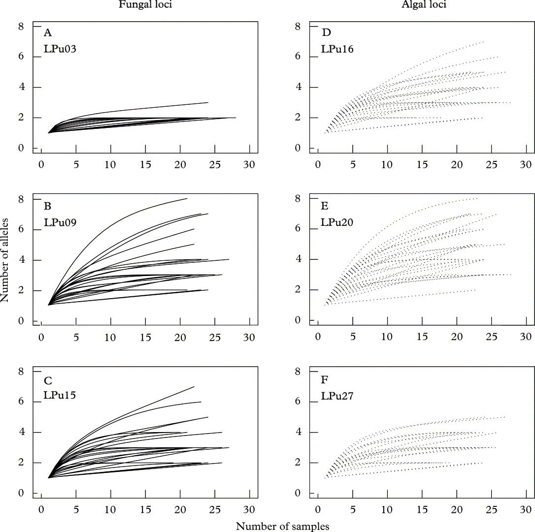
Fig. 1. Rarefaction curves for microsatellite alleles from 26 populations of Lobaria pulmonaria. A – C, fungal loci LPu03, LPu09, and LPu15; D – F, algal loci LPu16, LPu20, and LPu27. The analysis was performed by rarefaction of alleles within populations. Algal loci (·······); fungal loci (——).
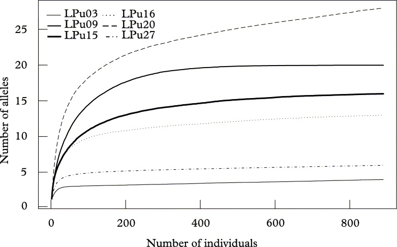
Fig. 2. Allelic accumulation curves, analogous to “species accumulation curves” sensu Gotelli & Colwell (Reference Gotelli and Colwell2001), showing the mean cumulative number of alleles (Sobs) of Lobaria pulmonaria or its photobiont from 500 replicate runs, relative to the number of individuals sampled across the landscape. Algal loci (broken lines); fungal loci (solid lines).

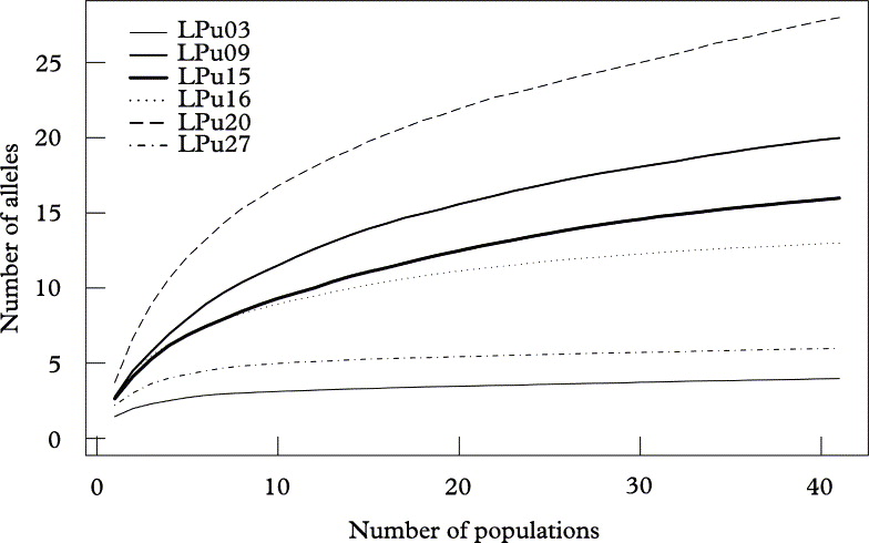
Fig. 3. Allelic accumulation curves, analogous to “species accumulation curves” sensu Gotelli & Colwell (Reference Gotelli and Colwell2001), showing the mean cumulative number of alleles (Sobs) of Lobaria pulmonaria or its photobiont from 500 replicate runs, relative to the number of sampled populations. Algal loci (broken lines); fungal loci (solid lines).
Indeed, for the fungal locus LPu15 and the photobiont loci LPu16 and LPu20, increased sampling effort might add 2·5–3·0%, 1·9–8·9% and 18·7–41·3% new alleles, respectively, as revealed by the nonparametric estimators of total richness ACE and Chao1 (Table 1). For the remaining loci, increased sampling effort was unlikely to detect new alleles.
Table 1. Number of alleles observed (Nr. alleles) and nonparametric estimators of allelic diversity (ACE, Chao1) in microsatellite loci of Lobaria pulmonaria (LPu03, LPu09, LPu15) and its photobiont (LPu16, LPu20, LPu27)

* ACE and Chao1 give the estimated total number of alleles.
† Miss_ACE and Miss_Chao1 give the percentage of alleles for the ACE and Chao1 estimators which might be revealed with additional sampling.
At the landscape level, loci reached saturation after about 400 individuals, with the exception of the high diversity locus LPu20 (Fig. 2). However, when resampling populations, only the two loci with the lowest diversity (i.e., LPu03, LPu27) reached saturation, while all other loci showed a more or less continuous increase in allelic numbers with the number of populations, implying that more than 41 populations would be required for a complete sampling of the allelic diversity of photobionts and mycobionts in the studied landscape (Fig. 3).
Discussion
The main purpose of this work was to estimate whether the sampling intensities required to characterize allelic diversity differed among mycobiont and photobiont populations, using the example of the epiphytic lichen Lobaria pulmonaria. I found that while overall diversity patterns were similar among photobiont and mycobiont, it appeared that the photobiont required a slightly higher sampling intensity than the mycobiont with respect to sampling within populations.
The sampling underestimated the total number of alleles in particular in the photobiont. Due to the high polymorphism of two photobiont loci (LPu16, LPu20), additional sampling might have revealed a substantial increase in the number of alleles, highlighting that photobionts of L. pulmonaria exhibited a higher genetic diversity than the mycobiont. In contrast, in the loci with low variability, the resampling curves flattened off early due to the lack of rare alleles. If the aim of a study were to recover as many alleles in a population as possible, then the sampling effort required to achieve this would need to be higher for the photobiont than for its mycobiont partner. To infer the pattern of genetic differentiation among populations situated within a landscape or a region, about 25–30 populations should be a large enough number to characterize a substantial part of the genetic variability of both fungal and algal populations. However, for most of the highly variable microsatellite loci, for an exhaustive sampling of alleles, a far larger number of populations would be required (i.e., >40), similar for algal and fungal loci. At the landscape scale, 300–400 individuals seem to be sufficient to sample the majority of alleles in L. pulmonaria and its photobiont. Within populations, photobiont populations require a slightly larger sampling effort (at least 30 individuals) than fungal populations (about 20 samples). Interestingly, the number inferred for the fungi does not seem to depend on the marker type. Zoller et al. (Reference Zoller, Lutzoni and Scheidegger1999) conducted resampling of DNA-sequence haplotypes of the combined ITS and LSU regions for samples collected from my study area (Marchairuz); within 22 thalli, an asymptote had been reached in this population, a number which is similar to that found for the far more variable microsatellite markers in the present study. Moreover, the required number is of a comparable magnitude relative to that of about 30 individuals per population recommended by Lindblom (Reference Lindblom2009) for populations of Xanthoria parietina, determined using DNA-sequence haplotypes. My overall recommendation is therefore to use at least 30 individuals per photobiont population, and at least 20 individuals per fungal population, whenever funding and time permit. From the study of Printzen et al. (Reference Printzen, Ekman and Tønsberg2003), who used DNA sequence haplotypes, it becomes obvious that far more individuals are required to resolve regional-scale haplotype diversities. For instance, in the Pacific Northwest, even after sampling 200 samples, the inclusion of additional individuals continued to add new haplotypes.
It is important to note that if the aim of a study is a comparison of photobiont and mycobiont genetic structures or diversities, it is most appropriate to sample the same number of individuals, and use the exact same thalli for genetic sampling of photobionts and mycobionts. In this particular case, analysis of photobionts and mycobionts from 30 thalli is recommended. Tied fungal-algal allelic data are optimal because they allow the exclusion of any differences found that are merely due to dissimilar or unbalanced sampling in space. It is unlikely that the sample sizes recommended above would be sufficient for areas which host a larger genetic diversity than the Central European biota investigated in the present data set that still exhibit strong signs of the depauperating effects of the Quaternary glaciations (Hewitt Reference Hewitt1996, 2000). More studies should be performed to test whether the sample sizes recommended here also hold for other geographic regions.
While I intended to give some recommendations for future studies on the approximate number of samples required to depict accurately allelic variability in populations of lichen-forming fungi and their photobionts, I would like to emphasize that sample sizes for population genetic studies ultimately depend on the aim of the study, the research question, the spatial scale of interest, and on the type of analysis to be applied to the data.
For instance, the analysis of fine-scale spatial genetic patterns requires particularly large sample sizes at the population level (Wagner et al. Reference Wagner, Holderegger, Werth, Gugerli, Hoebee and Scheidegger2005; Werth et al. Reference Werth, Wagner, Holderegger, Kalwij and Scheidegger2006). If the aim of a study is to resolve the fine-scale probability of clonal identity (e.g., among branches of a tree), or fine-scale gene diversity, then the sample size recommended above might be on the lower end. In these cases, it would be desirable to considerably increase the number of individuals sampled within a population, and sample fewer populations. For instance, studies of fine-scale genetic structure typically sample more than 100 individuals from one or very few populations for plants (Chung et al. Reference Chung, Nason and Chung2005; Dutech et al. Reference Dutech, Sork, Irwin, Smouse and Davis2005; Jones et al. Reference Jones, Vaillancourt and Potts2006; Yamagishi et al. Reference Yamagishi, Tomimatsu and Ohara2007) or fungi (Linde et al. Reference Linde, Zhan and McDonald2002). The required sampling effort critically depends on the spatial scale of interest. Thus, if a comparison among forest patches colonized by a lichen is intended, a different (and spatially less exhaustive) sampling scheme will be necessary than if subpopulations of a lichen occupying different branches within a tree are to be compared. If the aim is to resolve the rangewide patterns of genetic differentiation in a species, few individuals per population would suffice (e.g., 3–10), but many populations should be sampled across the entire range.
Allele-frequency based statistics such as classic F-statistics that measure genetic differentiation among populations do not require all alleles in a population to be sampled. Instead, they require a random sample drawn from the population, large enough to be representative of the allele frequency (Balding et al. Reference Balding, Bishop and Cannings2007). Under an allele frequency framework, within-population sample sizes may be smaller than recommended above, but it needs to be considered that larger sample sizes increase the statistical power to detect significant differentiation.
It is also noteworthy that for hierarchical analyses of molecular variance (AMOVA), a widely used technique to partition the genetic variance across various hierarchical levels, it is generally advisable to increase the number of populations sampled per group, relative to the number of individuals sampled per population (Fitzpatrick Reference Fitzpatrick2009). The aim of a hierarchical AMOVA is usually to test for differentiation among several groups of populations. Due to the nature of the permutation process used to test for statistical significance, sampling more individuals per population does not increase the statistical power of a hierarchical AMOVA at the group level (Fitzpatrick Reference Fitzpatrick2009). Fitzpatrick (Reference Fitzpatrick2009) presents an R script to determine the power of AMOVA for any hierarchical sampling scheme, which might be very useful for study design.
Also analyses that are based on the coalescent do not require complete sampling of alleles. On the contrary, in many situations it may not be advisable to use a large number of samples per population for such analyses; few samples per population but many loci are often a far better choice (Nordborg Reference Nordborg, Balding, Bishop and Cannings2001). Also, most coalescent-based methods do not advise the employment of a large number of populations, as the analyses may become increasingly computationally intensive, while adding little information (Nordborg Reference Nordborg, Balding, Bishop and Cannings2001). For instance, to estimate the number of migrants with the software MIGRATE-n (Beerli & Felsenstein Reference Beerli and Felsenstein2001), it is not advisable to use more than about 8 populations, and 30–50 individuals per population are usually sufficient (P. Beerli, personal communication).
Nested Clade Analysis (Templeton Reference Templeton1998), a method that has been widely used in phylogeographic studies, is sensitive to sample size and the completeness of haplotype sampling. Here, large (at best range-wide) geographic areas and as many populations as possible should be sampled to increase statistical power, whereas sample sizes within populations do not need to be large (Templeton Reference Templeton1998, Reference Templeton2004).
Ultimately, the optimal sample sizes for population-genetic analyses of photobionts and mycobionts depend on the research question in mind and on the analytical framework to be applied to the data.
I thank Ivo Widmer and Francesco Dal Grande for kindly sharing their findings on the specificity of the microsatellites developed for Lobaria pulmonaria, and I am grateful to Christoph Scheidegger for stimulating discussions. The project was funded by the Swiss National Foundation (PBBEA-111207, 3100AO-105830, and 31003A_1276346/1).