


1. INTRODUCTION
Study of intense laser propagating through plasma is of interest for wide range of applications, such as laser wakefield acceleration (Tajima & Dawson, Reference Tajima and Dawson1979; Jha et al., Reference Jha, Kumar, Upadhand and Raj2005), plasma based light source (Mori, Reference Mori1993), X-ray laser (Amendt et al., Reference Amendt, Eder and Wilks1991; Lemoff et al., Reference Lemoff, Yin, Gordan, Barty and Harris1995), optical harmonic generation (Sprangle et al., Reference Sprangle, Esarey and Ting1990; Lin et al., Reference Lin, Chen and Kieffer2002), inertial confinement fusion (Tabak et al., Reference Tabak, Hammer, Glinsky, Kruer, Wilks, Woodworth, Campbell, Perry and Mason1994), and so on. These applications provide strong motivation to encourage the studying of laser-plasma interaction, so this area has always been a fundamental topic in theoretical plasma physics in the past decades. On the other hand, owing to the generation of a hundred megaguass quasi-static magnetic field in laser plasma interaction (Gorbunov et al., Reference Gorbunov, Mora and Antonsen1997), the analysis of laser interaction with magnetized plasma was always an important issue for a real plasma system.
The harmonic generation is a nonlinear phenomenon in which the electrons oscillating in high-intensity laser fields is surveyed and assessed as a means of producing short-wavelength radiation sources. This phenomenon engaged scientists to clarify the mechanisms and methods of high-order harmonic generation.
Recently, high-order nonlinear effects have attracted great attention with the development of ultrafast laser technology. When we focus on an intense laser pulse into a gas, strong nonlinear interactions can lead to the generation of very high odd harmonics of the optical frequency of the pulse (Corkum, Reference Corkum1993; Salieres & Lewenstein, Reference Salieres and Lewenstein2001). This effect typically occurs at optical intensities on the order of 1014 W/cm2 or higher. Although only a tiny fraction of the laser power can be converted into higher harmonics, this output can still be useful for technical applications (Kienberger, Reference Kienberger, Goulielmakis, Uiberacker, Baltuska, Yakovlev, Bammer, Scrinzi, Westerwalbesloh, Kleineberg, Heinzmann, Drescher and Krausz2004).
The previous reports indicated that only the odd harmonics can be generated in the laser interaction with homogenous plasma (Esarey et al., Reference Esarey, Ting, Sprangle, Umsladter and Liu1993; Gibbon, Reference Gibbon1997; Mori et al., Reference Mori, Decker and Leemans1993; Wilks et al., Reference Wilks, Kruer and Mori1993), however, in the presence of a modulated transverse magnetic field, the phase-match second harmonic generation has been investigated (Rax & Fisch, Reference Rax and Fisch1992). Beside, the phase-mismatch second harmonic generation has been reported for the laser field interaction with underdense transversely magnetized plasma (jha et al., Reference Jha, Mishra, Raj and Upadhyay2007).
When a strong magnetic field applied into a plasma, the electron dynamic modified, and this leads to the nonlinear current modification. Therefore, it is reasonable that the magnetic field makes affect the harmonics generation. When the density perturbation produced by magnetic field coupled with electron quiver motions, it is plausible to generate the second harmonic (jha et al., Reference Jha, Mishra, Raj and Upadhyay2007).
In this paper, we investigate the phase-mismatch second and third harmonics generation in the interaction of intense laser beam and transversely magnetized plasma, when the plasma is dense and applied, magnetic field is strong. This report may be applicable in the wide range of external magnetic field strength and plasma density, in contrast to the pervious report for second harmonic generation that has been performed for underdense weakly magnetized plasma in the absence of the polarization field (jha et al., Reference Jha, Mishra, Raj and Upadhyay2007).
This paper is organized in four section. In Section 2, by using the perturbative technique in mildly relativistic and weakly nonlinear regime (a 1 < 1), induced nonlinear current density due to the interaction of intense laser beam with transversely magnetized plasma is derived for the second and third harmonics. In Section 3, the nonlinear wave equation solved for vector potential of driving laser beam, and the conversion efficiencies are obtained for the phase-mismatch second and third harmonics. Finally, a summary and conclusion is presented in Section 4.
2. NON-LINEAR CURRENT DENSITY
We assume the linearly polarized vector potential for nth harmonic is given as:
Here, A n, nω0 and k n = (nω0/c)εn1/2 are the amplitude, frequency, and wavevector of the nth harmonic, in which the εn introduces the dielectric permittivity at frequency nω0. The fundamental harmonic characteristics yield with n = 1.
We know the motion of charge particles in the presence of the intense laser beam and external magnetic field are described by relativistic Lorentz equation as:
Here E 1 is the laser field amplitude, ![]() and
and ![]() are the magnetic field of propagating laser beam and external magnetic field, respectively. Additionally,
are the magnetic field of propagating laser beam and external magnetic field, respectively. Additionally, ![]() is the polarization field due to the charge separation, and γ = (1 + p 2 /m 2c 2)1/2 is the relativistic factor. The ponderomotive force
is the polarization field due to the charge separation, and γ = (1 + p 2 /m 2c 2)1/2 is the relativistic factor. The ponderomotive force ![]() pushes the electrons in the direction of the laser beam propagation and the polarization field E z generated owing to the charge separation in the z direction. Furthermore, the force
pushes the electrons in the direction of the laser beam propagation and the polarization field E z generated owing to the charge separation in the z direction. Furthermore, the force ![]() , which arises to the external magnetic field has a component in the z direction, and so the strong magnetic field can be affect the charge separation efficiently. However, the ponderomotive force is smaller in plan wave with respect to the Gaussian profile short pulse beam, but for strongly magnetized plasma the influence of the z component of the force
, which arises to the external magnetic field has a component in the z direction, and so the strong magnetic field can be affect the charge separation efficiently. However, the ponderomotive force is smaller in plan wave with respect to the Gaussian profile short pulse beam, but for strongly magnetized plasma the influence of the z component of the force ![]() is very dominate for the charge separation process and the polarization field generation.
is very dominate for the charge separation process and the polarization field generation.
Using the perturbative theory in Eq. (2), and continuity equation (![]() ), it is possible to expand all quantities in terms of the order of the radiation field. In this method, the relativistic effect comes into play in the third order velocity components and higher. If we consider the plasma is cold and the electrons are at rest before the laser field is applied, the first order equations for the electron velocity components, in accord to this technique, is written as:
), it is possible to expand all quantities in terms of the order of the radiation field. In this method, the relativistic effect comes into play in the third order velocity components and higher. If we consider the plasma is cold and the electrons are at rest before the laser field is applied, the first order equations for the electron velocity components, in accord to this technique, is written as:

where E z(1), E 1 = −∂A 1/∂t, ωc = eB 0/m, are the first order perturbation for polarization field, laser field amplitude, and the electron cyclotron frequency, respectively. By taking a time derivative of the second relation in Eq. (3), also using the first relation, and estimate the relative term to the first order of the polarization field (∂E z(1)/∂z = −e n (1)/ε0) as below:
![\eqalign{ - {e \over m}{\partial \over \partial t} E_z^{\lpar 1\rpar} & = {e^2 \over m{\rm \epsilon}_0} {\partial \over \partial t} n^{\lpar 1\rpar} dz \cr & =- {e^2 \over m{\rm \epsilon}_0} \left[{\partial \over \partial z} \lpar n_0 v_z^{\lpar 1\rpar }\rpar \right] dz = - {\rm \omega}_p^2 v_z^{\lpar 1\rpar}\comma \;}](https://static.cambridge.org/binary/version/id/urn:cambridge.org:id:binary:20151021072132278-0431:S0263034612000092_eqn4.gif?pub-status=live)
we arrive
where a 1 = eE 1/mcω0, ωp = (ne 2/mε0)1/2, and n 0 are the normalized laser field amplitude (or normalized vector potential a 1 = eA 1/mc), plasma frequency, and unperturbed electron density, respectively, also φ = k 1z − ω0t. Eq. (4) indicates that the polarization field oscillates as the same frequency with v z(1), or the laser field frequency. This means that the polarization field is not slow and it is reasonable that this field makes affect the harmonic generation. The solution of Eq. (5) and performing the same steps for component v x, the first order electron velocity components are given by:

By following the same steps for the nth harmonic, the first order velocity components yield only by substituting ω0 → nω0, a 1 → a n and φ → k nz − nω0t, into Eq. (6). Therefore, the linear part of the induced current density corresponding to the nth harmonic, J x(1)(nω0) = −n 0e v x(1)(nω0), can be written as:

where a n = eA n/mc is the normalized vector potential for nth harmonic. Substituting Eq. (7) into the wave equation for nth harmonic, it is possible to derive the linear dispersion equation as:

Using Eq. (8) into the well known transverse wave dispersion equation k n = (nω0/c)εn1/2, the plasma permittivity corresponding to the frequency nω0 is given by:

It is important to note that, the effect of polarization field is included in deriving the Eq. (9).
It is intuitively understood that electron density is disturbed when a driving laser beam propagate through the plasma. The spatiotemporal variations for electron perturbations are given by the continuity equation. Therefore, similarly to the velocity components, we can expand the electron density in terms on the order of the radiation field. Then in accordance to the continuity equation and Eq. (6), the first order electron density perturbation takes the form as:
Now, we are on the stage to obtain the second order velocity components. In doing so, similar to the first order, by the same procedure the coupled equations arise from the relativistic Lorentz equation are given by:

where E z(2) is the second order perturbation for polarization field. After some mathematical processes, we arrive to the following partial differential equation for the z component of the second order of the electron velocity as:
![\eqalign{& {{\partial ^2 v_z^{\lpar 2\rpar } } \over {\partial t^2 }}+{\rm \omega}_p^2 v_z^{\lpar 2\rpar }+{\rm \omega}_c^2 v_z^{\lpar 2\rpar }=- {{a_1^2 c^2\, k_1 {\rm \omega}_0 {\rm \omega}_c^2 \lpar {\rm \omega}_p^2+{\rm \omega}_c^2\rpar } \over {2\lpar {\rm \omega}_0^2 - {\rm \omega}_p^2 - {\rm \omega}_c^2\rpar ^2 }} \cr &\quad +{{a_1^2 c^2\, k_1 {\rm \omega}_c \left[{2\lpar {\rm \omega}_0^2 - {\rm \omega}_p^2\rpar ^2 - {\rm \omega}_c^2 \lpar 4{\rm \omega}_0^2 - {\rm \omega}_p^2+{\rm \omega}_c^2\rpar } \right]} \over {2\lpar {\rm \omega}_0^2 - {\rm \omega}_p^2 - {\rm \omega}_c^2\rpar ^2 }}\cos2{\rm \varphi} .}](https://static.cambridge.org/binary/version/id/urn:cambridge.org:id:binary:20151021072132278-0431:S0263034612000092_eqn12.gif?pub-status=live)
The solution of Eq. (12) give us the component v z(2), so by the same procedure it is possible to find the component v x(2). Therefore, the second order velocity components, easily, find as:
![\eqalign{ v_x^{\lpar 2\rpar }&={{a_1^2 c^2\, k_1 {\rm \omega}_c \big[ \lpar {\rm \omega}_0^2 - {\rm \omega}_p^2\rpar ^2 - {\rm \omega}_c^2 \lpar 4{\rm \omega}_0^2 - {\rm \omega}_p^2\rpar \big] } \over {2\lpar {\rm \omega}_0^2 - {\rm \omega}_p^2 - {\rm \omega}_c^2\rpar ^2 \lpar 4{\rm \omega}_0^2 - {\rm \omega}_p^2 - {\rm \omega}_c^2\rpar }}\sin 2{\rm \varphi} \cr v_z^{\lpar 2\rpar }&=- {{a_1^2 c^2\, k_1 {\rm \omega}_c^2 {\rm \omega}_0 \lpar {\rm \omega}_p^2+{\rm \omega}_c^2\rpar } \over {2\lpar {\rm \omega}_0^2 - {\rm \omega}_p^2 - {\rm \omega}_c^2\rpar ^2 }} \cr &\quad - {{a_1^2 c^2\, k_1 {\rm \omega}_0 \big[ 2\lpar {\rm \omega}_0^2 - {\rm \omega}_p^2\rpar ^2 - {\rm \omega}_c^2 \lpar 4{\rm \omega}_0^2 - {\rm \omega}_p^2+{\rm \omega}_c^2\rpar \big] } \over {2\lpar {\rm \omega}_0^2 - {\rm \omega}_p^2 - {\rm \omega}_c^2\rpar ^2 \lpar 4{\rm \omega}_0^2 - {\rm \omega}_p^2 - {\rm \omega}_c^2\rpar }}\cos2{\rm \varphi} . }](https://static.cambridge.org/binary/version/id/urn:cambridge.org:id:binary:20151021072132278-0431:S0263034612000092_eqn13.gif?pub-status=live)
It is clear from Eq. (13), the second order velocity components oscillate with frequency twice the laser field frequency. This effect arises from the external magnetic field, and coupling between the external and propagating magnetic fields.
The second order electron density perturbation is derived by the same method presented for n (1) as:

Finally, we can expand the Lorentz equation in terms of the third order of the radiation field. Note that in this case, the relativistic factor play an important role in electron dynamic. The coupled equations for velocity components written as:

where E z(3) and γ(2) = [(v x(1))2 + (v z(1))2]/2c 2 are the third order perturbation for polarization field and the relativistic factor. By using some careful mathematical processes, similar to the first and second orders, we will get to the following results for the third order velocity components as:
![\eqalign{ v_x^{\lpar 3\rpar } &=- {{a_1^3 c} \over {8\lpar {\rm \omega}_0^2 - {\rm \omega}_p^2 - {\rm \omega}_c^2\rpar ^3 }}\left[{{A_{\rm \varphi}+{\rm \omega}_c^2 B_{\rm \varphi} } \over {\lpar {\rm \omega}_0^2 - {\rm \omega}_p^2 - {\rm \omega}_c^2\rpar }}\sin {\rm \varphi}\right. \cr &\left. \quad +{{A_3 {\rm \varphi}+{\rm \omega}_c^2 B_3 {\rm \varphi} } \over {\lpar 9{\rm \omega}_0^2 - {\rm \omega}_p^2 - {\rm \omega}_c^2\rpar }}\sin 3{\rm \varphi} \right]\cr v_z^{\lpar 3\rpar } &={{a_1^3 c} \over {8\lpar {\rm \omega}_0^2 - {\rm \omega}_p^2 - {\rm \omega}_c^2\rpar ^3 }}\left[{{C_{\rm \varphi}+D_{\rm \varphi} } \over {\lpar {\rm \omega}_0^2 - {\rm \omega}_p^2 - {\rm \omega}_c^2\rpar }}\cos{\rm \varphi}\right. \cr &\left. \quad +{{C_3 {\rm \varphi}+D_3 {\rm \varphi} } \over {\lpar 9{\rm \omega}_0^2 - {\rm \omega}_p^2 - {\rm \omega}_c^2\rpar }}\cos3{\rm \varphi} \right]\comma \; }](https://static.cambridge.org/binary/version/id/urn:cambridge.org:id:binary:20151021072132278-0431:S0263034612000092_eqn16.gif?pub-status=live)
where,

In view of the fact that the harmonics are driven by the nonlinear current, we can evaluate this source term using the perturbed quantities obtained previously. According to the current density carried by the electrons J = −nev, the second order nonlinear current density for the second harmonic, J x(2) = −e(n 0v x(2) + n (1)v x(1)), after substituting the required quantities, written as:

To proceed further, we find the third order current density for third harmonic, J x(3) = −e(n 0v x(3) + n (1)v x(2) + n (2)v x(1)) as:
![\eqalign{J_x^{\lpar 3\rpar } \lpar 3{\rm \omega}_0\rpar &={{a_1^3 n_0 ec} \over {8\lpar {\rm \omega}_0^2 - {\rm \omega}_p^2 - {\rm \omega}_c^2\rpar ^3 \lpar 9{\rm \omega}_0^2 - {\rm \omega}_p^2 - {\rm \omega}_c^2\rpar }} \cr & \quad\times \left[{\left({A_{3{\rm \varphi} }^\prime+{{c^2\, k_1^2 } \over {\lpar 4{\rm \omega}_0^2 - {\rm \omega}_p^2 - {\rm \omega}_c^2\rpar }}B_{3{\rm \varphi} }^\prime } \right)\sin 3{\rm \varphi} } \right]\comma \;}](https://static.cambridge.org/binary/version/id/urn:cambridge.org:id:binary:20151021072132278-0431:S0263034612000092_eqn18.gif?pub-status=live)
where,

3. CONVERSION EFFICIENCY
The above expressions for the harmonic components of the source current, J x(2)(2ω0) and J x(3)(3ω0), can be used in the following wave equation, to determine the growth of harmonics radiation.

where subscript n refers to the order of harmonic. We obtained this source term in the previous section, thus the vector potential amplitude can be evaluate by solution the wave equation. The steady state amplitude for the phase-mismatch second harmonic obtained by suggestion a 2 = a 2(z)e i(k 2z−2ω0t)/2 + c.c into Eq. (19), and making used of the Eq. (17).
Assuming that ∂2a 2(z)/∂z 2≪k 2∂ a 2(z)/∂z, which means that ∂a 2(z)/∂z changes appreciably larger than wavelength 2π/k 2, and for 4ω02≫ωc2 , we arrive the normalized amplitude for the phase-mismatch second harmonic as below:
![\eqalign{ a_2 \lpar z\rpar &={{3a_1^2 {\rm \omega}_c } \over {16c}}{{{\rm \omega}_p^2 } \over {{\rm \omega}_0^2 }} \cr &\quad\times {{\mathop {\left[{1 - {{{\rm \omega}_p^2 } \over {{\rm \omega}_0^2 }}\left({1 - {{{\rm \omega}_p^2 } \over {{\rm \omega}_0^2 }}} \right)\mathop {\left({1 - {{{\rm \omega}_c^2 } \over {{\rm \omega}_0^2 }} - {{{\rm \omega}_p^2 } \over {{\rm \omega}_0^2 }}} \right)}\nolimits^{ - 1} } \right]}\nolimits^{1/2} } \over {\mathop {\left[{1 - {{{\rm \omega}_p^2 } \over {4{\rm \omega}_0^2 }}\left({1 - {{{\rm \omega}_p^2 } \over {4{\rm \omega}_0^2 }}} \right)\mathop {\left({1 - {{{\rm \omega}_c^2 } \over {4{\rm \omega}_0^2 }} - {{{\rm \omega}_p^2 } \over {4{\rm \omega}_0^2 }}} \right)}\nolimits^{ - 1} } \right]}\nolimits^{1/2} }} \cr & \quad \times {{\left({1 - {{{\rm \omega}_p^2 } \over {{\rm \omega}_0^2 }}+{{{\rm \omega}_c^2 } \over {{\rm \omega}_0^2 }}} \right)} \over {\mathop {\left({1 - {{{\rm \omega}_p^2 } \over {{\rm \omega}_0^2 }} - {{{\rm \omega}_c^2 } \over {{\rm \omega}_0^2 }}} \right)}\nolimits^2 \left({1 - {{{\rm \omega}_p^2 } \over {4{\rm \omega}_0^2 }} - {{{\rm \omega}_c^2 } \over {4{\rm \omega}_0^2 }}} \right)}} \cr &\quad \times e^{i\lpar \Delta kz\rpar /2} \left({{{\sin\!\lpar \Delta k.z/2\rpar } \over {\Delta k}}} \right)\comma \; }](https://static.cambridge.org/binary/version/id/urn:cambridge.org:id:binary:20151021072132278-0431:S0263034612000092_eqn20.gif?pub-status=live)
where Δk = 2k 1 − k 2 is the wavevector mismatch for the second harmonic. Definitely, anyone find from Eq. (20) that the second harmonic can be generate only in the magneto-active plasmas, which may be considered as an important advantage for such kind of plasmas.
The normalized amplitude for the phase-mismatch third harmonic is obtained by the same procedure, by substituting a 3 = a 3(z)e i(k 3z−3ω0t)/2 + c.c into Eq. (19) and using the Eq. (18), for 9ω02 ≫ ωc2. The result is given by:
![\eqalignno{ a_3 \lpar z\rpar =&{{{\rm \omega}_p^2 a_1^3 } \over {24{\rm \omega}_0 c}} \left[1 - {{{\rm \omega}_p^2 } \over {9{\rm \omega}_0^2 }}\left(1 - {{{\rm \omega}_p^2 } \over {9{\rm \omega}_0^2 }} \right)\right. \left(1 - {{{\rm \omega}_c^2 } \over {9{\rm \omega}_0^2 }} - {{{\rm \omega}_p^2 } \over {9{\rm \omega}_0^2 }} \right)^{ - 1} \bigg]^{ - 1/2} \cr & \times \left\{{\matrix{ \displaystyle{{A_{3{\rm \varphi} }^\prime } \over {{\rm \omega}_0^8 }}+\left[1 - {{{\rm \omega}_p^2 } \over {{\rm \omega}_0^2 }}\left(1 - {{{\rm \omega}_p^2 } \over {{\rm \omega}_0^2 }} \right)\left(1 - {{{\rm \omega}_c^2 } \over {{\rm \omega}_0^2 }} - {{{\rm \omega}_p^2 } \over {{\rm \omega}_0^2 }} \right)^{ - 1} \right]\cr \left(4 - \displaystyle{{{\rm \omega}_p^2 } \over {{\rm \omega}_0^2 }} - {{{\rm \omega}_c^2 } \over {{\rm \omega}_0^2 }} \right)^{ - 1} \times \displaystyle{{B_{3{\rm \varphi} }^\prime } \over {{\rm \omega}_0^8 }}} \over \left(1 - \displaystyle{{{\rm \omega}_p^2 } \over {{\rm \omega}_0^2 }} - {{{\rm \omega}_c^2 } \over {{\rm \omega}_0^2 }} \right)^3 \left(9 - \displaystyle{{{\rm \omega}_p^2 } \over {{\rm \omega}_0^2 }} - {{{\rm \omega}_c^2 } \over {{\rm \omega}_0^2 }} \right)} \right\}\cr & \times e^{i\lpar \Delta k^\prime z\rpar /2} \left({{{\sin\!\lpar \Delta k^\prime .z/2\rpar } \over {\Delta k^\prime }}} \right)\comma \;}](https://static.cambridge.org/binary/version/id/urn:cambridge.org:id:binary:20151021072132278-0431:S0263034612000092_eqn21.gif?pub-status=live)
where Δk′ = 3k 1 − k 3 is the wavevector mismatch for the third harmonic. Taking into account that the conversion efficiency for nth harmonic is defined as:

we get the conversion efficiencies for the phase-mismatch second and third harmonics as below:
![\eqalign{{\rm \eta}_2 \lpar z\rpar &= {9a_1^2 {\rm \omega}_c^2 \over 128c^2} {{\rm \omega}_p^4 \over {\rm \omega}_0^4} {\left[\matrix{1 - \displaystyle{{\rm \omega}_p^2 \over {\rm \omega}_0^2} \left(1 - {{\rm \omega}_p^2 \over {\rm \omega}_0^2} \right)\cr \left(1 - \displaystyle{{\rm \omega}_c^2 \over {\rm \omega}_0^2} - {{\rm \omega}_p^2 \over {\rm \omega}_0^2} \right)^{ - 1}} \right]^{1/2} \over \left[\matrix{1 - \displaystyle{{\rm \omega}_p^2 \over 4{\rm \omega}_0^2} \left(1 - {{\rm \omega}_p^2 \over 4{\rm \omega}_0^2} \right)\cr \left(1 - \displaystyle{{\rm \omega}_c^2 \over 4{\rm \omega}_0^2} - {{\rm \omega}_p^2 \over 4{\rm \omega}_0^2} \right)^{ - 1}} \right]^{1/2}} \cr & \quad \times {\left(1 - \displaystyle{{\rm \omega}_p^2 \over {\rm \omega}_0^2} + {{\rm \omega}_c^2 \over {\rm \omega}_0^2} \right)^2 \over \left(1 - \displaystyle{{\rm \omega}_p^2 \over {\rm \omega}_0^2} - {{\rm \omega}_c^2 \over {\rm \omega}_0^2} \right)^4 \left(1 - \displaystyle{{\rm \omega}_p^2 \over 4{\rm \omega}_0^2} - {{\rm \omega}_c^2 \over 4{\rm \omega}_0^2} \right)^2} \cr &\quad \times \left({\sin^2\! \lpar \Delta k.z/2\rpar \over \lpar \Delta k\rpar ^2} \right).}](https://static.cambridge.org/binary/version/id/urn:cambridge.org:id:binary:20151021072132278-0431:S0263034612000092_eqn23.gif?pub-status=live)
![\eqalign{{\rm \eta}_3 \lpar z\rpar &= {{\rm \omega}_p^4 a_0^4 \over 192{\rm \omega}_0^2 c^2} {\left[\matrix{1 - \displaystyle{{\rm \omega}_p^2 \over {\rm \omega}_0^2} \left(1 - \displaystyle{{\rm \omega}_p^2 \over {\rm \omega}_0^2} \right)\cr \left(1 -\displaystyle {{\rm \omega}_c^2 \over {\rm \omega}_0^2} - {{\rm \omega}_p^2 \over {\rm \omega}_0^2} \right)^{ - 1}} \right]^{ - 1/2} \over \left[\matrix{1 - \displaystyle{{\rm \omega}_p^2 \over 9{\rm \omega}_0^2} \left(1 - \displaystyle{{\rm \omega}_p^2 \over 9{\rm \omega}_0^2} \right)\cr \left(1 - \displaystyle{{\rm \omega}_c^2 \over 9{\rm \omega}_0^2} - {{\rm \omega}_p^2 \over 9{\rm \omega}_0^2} \right)^{ - 1}} \right]^{1/2}} \cr &\quad\times {\left\{\matrix{\displaystyle{A_{3{\rm \varphi}}^{\prime} \over {\rm \omega}_0^8} + \left[1 - {{\rm \omega}_p^2 \over {\rm \omega}_0^2} \left(1 - {{\rm \omega}_p^2 \over {\rm \omega}_0^2} \right)\left(1 - {{\rm \omega}_c^2 \over {\rm \omega}_0^2} - {{\rm \omega}_p^2 \over {\rm \omega}_0^2} \right)^{ - 1} \right]\cr \left(4 - \displaystyle{{\rm \omega}_p^2 \over {\rm \omega}_0^2} - {{\rm \omega}_c^2 \over {\rm \omega}_0^2} \right)^{ - 1} \times \displaystyle{B_{3{\rm \varphi}}^{\prime} \over {\rm \omega}_0^8}} \right\}^2 \over \left(1 - \displaystyle{{\rm \omega}_p^2 \over {\rm \omega}_0^2} - {{\rm \omega}_c^2 \over {\rm \omega}_0^2} \right)^6 \left(9 - \displaystyle{{\rm \omega}_p^2 \over {\rm \omega}_0^2} - {{\rm \omega}_c^2 \over {\rm \omega}_0^2} \right)^2} \cr &\quad \times \left({\sin^2\! \lpar \Delta k^{\prime} .z/2\rpar \over \lpar \Delta k^\prime\rpar ^2} \right).}](https://static.cambridge.org/binary/version/id/urn:cambridge.org:id:binary-alt:20160626073243-51430-mediumThumb-S0263034612000092_eqn24.jpg?pub-status=live)
With a short look at Eqs. (23) and (24), it is found that the harmonics oscillate in magnitude around an average value due to the dephasing between the pump laser and the radiation harmonics. The maximum conversion efficiencies take place in the coherence lengths z c = π/Δk and z′c= π/Δk′, respectively, for the second and third harmonics. Therefore, the power efficiencies are harmonic by z, so we have the points with maximum and minimum electric field amplitude for the radiation harmonics inside the plasma.
According to this fact that we deal with the strongly magnetized dense plasma, there is worry about that the laser beam may be damped or absorbed. The absorbtion occurs for ε1 → ∞ and or ω02 = ωp2 + ωc2, however, any damping takes place for ε1 < 0.
In Figure 1, we show the damping and absorbing regions on the (ωp/ω0 − ωc /ω0) plan. The hachured area predicts the damping region for the laser beam, while all points on the solid line satisfy the absorbtion condition. If the parameters ωp/ω0 and ωc/ω0 choose in such a manner that the corresponding point on the (ωp/ω0 − ωc/ω0) plan is placed on the region ε1 > 0, the laser beam does not damp or absorb during propagating through the plasma.

Fig. 1. (Color online) Schematic investigation for damping and absorbing region on the (ωp/ω0 − ωc/ω0) plan for the laser beam propagating through the plasma.
The conversion efficiency %η2 for the second harmonic is plotted as a function of z/λ for ωp/ω0 = 0.3, and for different values of the external magnetic field, in Figure 2. We assume the pump laser is a Nd:Yag laser with intensity around 1017 W/cm2 (a 1 = 0.271) and frequency ω0 = 1.88 × 10¹⁵s −1 and or wavelength λ = 1 µm. The figure shows the second harmonic efficiency reaches to the maximum value after that the laser beam traveling as coherence lengths 7.1 µm and 6.8 µm inside the plasma, respectively, for ωc/ω0 = 0.1 and ωc/ω0 = 0.2. Therefore, the coherence length for radiation harmonic decreases with magnetic field increasing. On the other hand, the figure demonstrates that the second harmonic conversion efficiency drastically increased with magnetic field increasing.
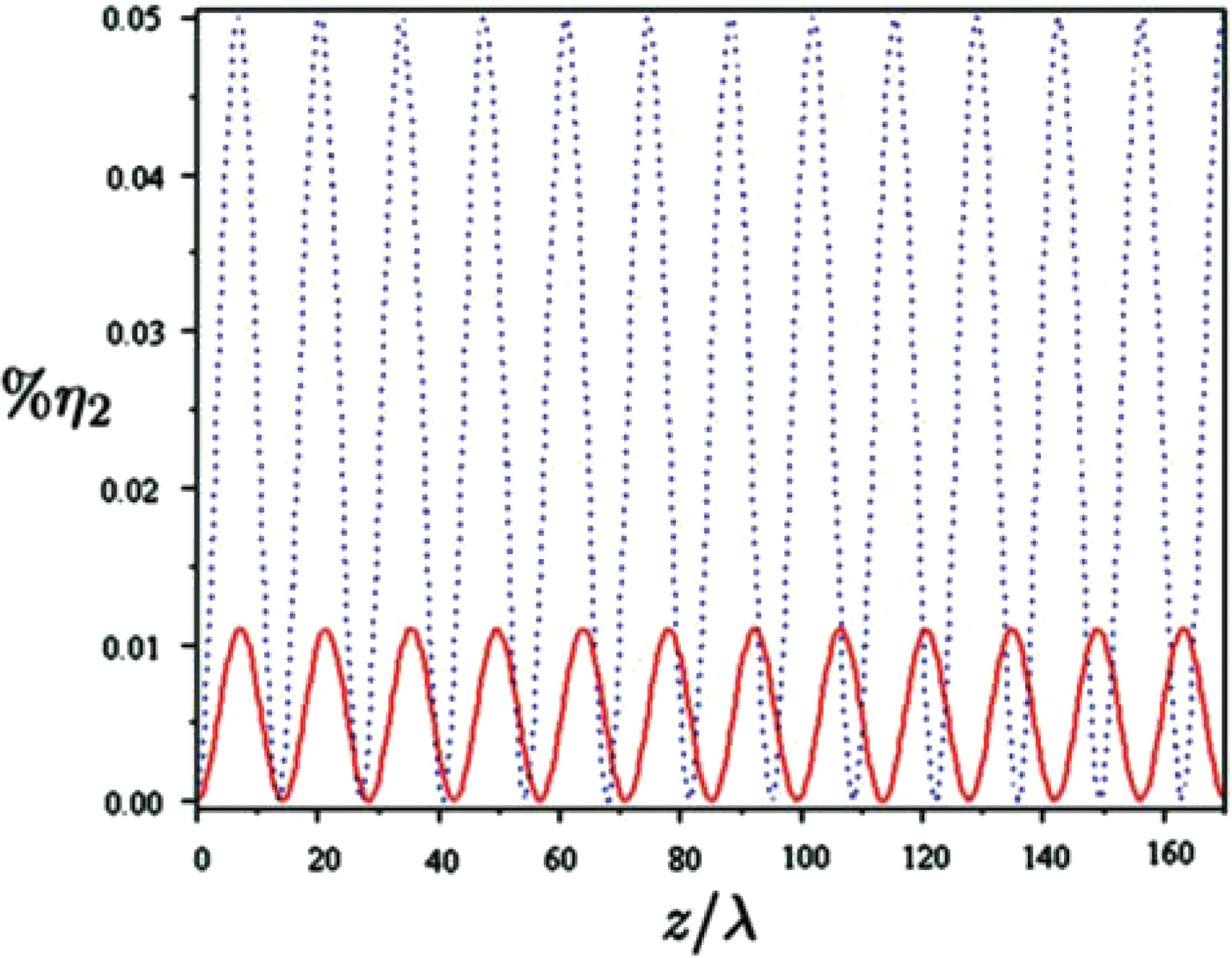
Fig. 2. (Color online) The phase-mismatch second harmonic conversion efficiency variation as a function of z/λ, for ωp/ω0 = 0.3, a 1 = 0.271. The solid line for ωc/ω0 = 0.1 and the point line for ωc/ω0 = 0.2.
Figure 3 indicates the second harmonic maximum conversion efficiency variation as a function of ωc/ω0, for various values of the plasma density. The figure reveals that the harmonic radiation is completely different for strongly magnetized plasma, in comparison to the weakly magnetized case (jha et al., Reference Jha, Mishra, Raj and Upadhyay2007). The difference arises for dense and strongly magnetized plasma, when the effect of the polarization field dominates. It is clear from Figure 3 for sufficiently strong magnetic field, the second harmonic generation scenario is changed. For example, for ωc/ω0 > 0.57, the second harmonic generation is stopped for ωp/ω0 = 0.6 and drastically increased for ωp/ω0 = 0.5, however, based on the previous report (jha et al., Reference Jha, Mishra, Raj and Upadhyay2007) the second harmonic generation increased continuously by increasing ωp/ω0 for a given magnetic field. Furthermore, the figure predicts that the harmonic radiation cuts off, when the magnetic field strength increases up until the saturation strength B sat. As the figure demonstrates, saturation strength decreases with density increasing.

Fig. 3. (Color online) The maximum conversion efficiency variation for the phase-mismatch second harmonic with respect to the ωc/ω0, for a 1 = 0.271, respectively, the solid line for ωp/ω0 = 0.6, the dash dot line for ωp/ω0 = 0.5.
In Figure 4, the maximum power efficiency variation plotted as a function of parameter ωp/ω0, for different values of magnetic field strength. The figure shows that for a constant magnetic field, the harmonic generation grows with density increasing. However, the harmonic radiation cuts-off, when the plasma density increases up until the saturation density n sat. The saturation density depends on the applied magnetic field strength and increases for the weak magnetic field.

Fig. 4. (Color online) The maximum conversion efficiency variation for the phase-mismatch second harmonic with respect to the ωp/ω0, for a 1 = 0.271, respectively, the solid line for ωc/ω0 = 0.5, the dash dot line for ωc/ω0 = 0.6.
The conversion efficiency %η3 variation is plotted as a function z/λ, for the phase-mismatch third harmonic and for a non-magnetized plasma, in Figure 5. However, the power efficiency is very small, but it is important to note that the third harmonic can be generate for the non-magnetized case. In this figure, the dot line shows the average conversion efficiency, while the dash dot line indicates the conversion efficiency for the phase-match third harmonic (Esarey et al., Reference Esarey, Ting, Sprangle, Umsladter and Liu1993; Gibbon, Reference Gibbon1997; Mori et al., Reference Mori, Decker and Leemans1993; Wilks et al., Reference Wilks, Kruer and Mori1993). Thus, the power efficiency slightly decreased for the phase-mismatch harmonic.

Fig. 5. (Color online) The phase-mismatch third harmonic conversion efficiency variation as a function of z/λ, for a non-magnetized plasma, ωp/ω0 = 0.6, a 1 = 0.271. The dot line shows the average phase-mismatch conversion efficiency and the dash dot line indicates the phase-matched conversion efficiency based on previous reports (Esarey et al., Reference Esarey, Ting, Sprangle, Umsladter and Liu1993; Gibbon, Reference Gibbon1997; Mori et al., Reference Mori, Decker and Leemans1993; Wilks et al., Reference Wilks, Kruer and Mori1993).
In Figure 6, we plot the maximum conversion efficiency variation for the third harmonic as a function of ωc/ω0, for various values of the plasma density. The figure shows that the harmonic radiation appreciably enhances by applying the external magnetic field. Like to the second harmonic, the third harmonic radiation stopped, when the magnetic field increased up to the saturation strength B sat. The saturation strength increases for the low density plasma.

Fig. 6. (Color online) The maximum conversion efficiency variation for the the phase-mismatch third harmonic with respect to the ωc/ω0, for a 1 = 0.271, respectively, the solid line for ωp/ω0 = 0.6, the dash dot line for ωp/ω0 = 0.5.
By tracking the values of the parameters ωp/ω0 and ωc/ω0, in one of the branches in Figures 3 and 6, anyone can find that the harmonics generation appreciably increase, when we get closest to the border line between ε1 < 0 and ε1 > 0, in Figure 1. For a point, which is exactly placed on the border line the harmonic generation stopped. Therefore, we can estimate the saturation magnetic field by making used of the condition ε1 = 0, as below:

where m and e, are the electron mass and charge, respectively.
Finally, the maximum conversion efficiency variation for the third harmonic is plotted as a function of ωp/ω0, for different values of magnetic field strength, in Figure 7. The figure shows that the harmonic radiation stopped, when the density increased up to the saturation density n sat, while the applied magnetic field remains constant. The saturation density varies with magnetic field strength and decreases for the stronger magnetic field. The saturation density is accessible according to the condition ε1 = 0, as:

where n cr = mε0 ω02 /e2 is the critical density.

Fig. 7. (Color online) The maximum conversion efficiency variation for the phase-mismatch third harmonic with respect to the ωp/ω0, for a 1 = 0.271, respectively, the solid line for ωc/ω0 = 0.5, the dash dot line for ωc/ω0 = 0.6.
4. SUMMARY AND CONCLUSION
In summary, we have investigated the conversion of a fraction of a laser beam to its second and third harmonics, in the interaction of intense laser field with transversely magnetized plasma. The plasma was dense and below the critical density, but the effect of the polarization field was considered. The harmonics radiation studied when there was a phase-mismatch between the phase velocities of the laser field and the generated harmonics. We proved the existence of a saturation magnetic field B sat, in which the harmonics radiation stopped for B ≥ B sat. The strength of saturation field depended on the plasma density and increased for the low density plasma. This result arose owing to the polarization field effect in strongly magnetized dense plasma, and has not been reported previously. It is shown that for B < B sat the harmonics radiation appreciably enhanced with magnetic field increasing, however, the second harmonic disappeared in the absence of the magnetic field. We have investigated the existence of saturation density n sat, where the harmonic radiation stopped for n ≥ n sat, while the applied magnetic field remained constant. In addition, we shown that for a non-magnetized plasma, the average phase-mismatch conversion efficiency was always a little below the phase-match one, for the third harmonic radiation. As a final, and important remark, it would be useful to note that, for sufficiently low density plasma we need a super strong magnetic field to get a maximum efficiency, so take into account that such strong field may be not accessible technically, we should be make a balance between the plasma density and the applied magnetic field to reach an optimum efficiency.


