


1. INTRODUCTION
Technological development in the field of laser physics has ushered a new era where highly intense lasers are available. This has opened new vistas of novel applications not only in other fields but also in plasmas such as plasma based accelerators (Esarey et al., 1996; Hartemann et al., Reference Hartemann, Van Meter, Troha, Landahl, Luhmann, Baldis, Gupta and Kerman1998; Sarkisov et al., Reference Sarkisov, Bychenkov, Novikov, Tikhonchuk, Maksimchuk, Chen, Wagner, Mourou and Umstadter1999; Hora et al., Reference Hora1988, Reference Hora, Hoeless, Scheid, Wang, Ho, Osman and Castillo2000; Hauser et al., Reference Hauser, Scheid and Hora1994), advanced laser fusion schemes (Tabak et al., Reference Tabak, Hammer, Glinsky, Kruer, Wilks, Woodworth, Campbell, Perry and Mason1994; Deutsch et al., Reference Deutsch, Furkawa, Mima, Murakami and Nishihara1996; Regan et al., Reference Regan, Bradley, Chirokikh, Craxton, Meyerhofer, Seka, Short, Simon, Town and Yaakobi1999), ionospheric radio wave propagation, X-ray lasers (Lemoff et al., Reference Lemoff, Yin, Gordon, Barty and Harris1995), harmonic generation (Sprangle et al., Reference Sprangle and Esarey1990) and new radiation sources (Benware et al., Reference Benware, Macchietto, Moreno and Rocca1998; Foldes et al., Reference Foldes, Bakos, Bakonyi, Nagy and Szatmari1999; Fedotov et al., Reference Fedotov, Naumov, Silin, Uryupin, Zheltikov, Tarasevitch and Von der Linde2000). To make these applications feasible, it is desirable that laser beam should propagate several Rayleigh lengths (R d). But in vacuum, the laser beam propagation is limited by diffraction characteristic distance R d ~ k 0 + a 02 +, where k 0+ is wavenumber and a 0+ is laser spot size in vacuum.
In a nonlinear medium like dielectrics, semiconductors and plasmas, the phenomenon of self-focusing being genuinely nonlinear optical process is induced by modification of refractive index of material to intense electromagnetic/laser beam. The electronic nonlinear response of a medium leads to nonlinear polarization that influences the propagation of beam itself. Usually for an electromagnetic radiation such as laser characterized by Gaussian intensity distribution, the refractive index of the medium increases with electric field intensity, leading to self-focusing of the beam. Historically, this phenomenon was predicted by Kerr in 1960 (Askaryan, Reference Askaryan1962; Chiao, Reference Chiao, Garmire and Townes1964) and experimentally verified. In such medium, refractive index is described by the formulae n = n 0 = n 2I, where n 0 and n 2 are linear and nonlinear coefficient of refractive index and I is intensity of radiation. Kerr induced self-focusing is relevant to many applications in laser physics (Chen & Wang, Reference Chen and Wang1991; Herrmann, Reference Herrmann1994). This phenomenon also predicted by Askaryan (Reference Askaryan1962) and named as self-focusing of radiation. The possibility of self-focusing or self-trapping of a laser beam in a solid has been further discussed by Chiao (Reference Chiao, Garmire and Townes1964). This nonlinearly generic process had been focus of attention for nearly five decades and is still being actively persued by researchers worldwide because of their relevance to a number of newly discovered processes. Hora (Reference Hora1969) treated the process of self-focusing due to the gradient of the light intensity. Basic nonlinear physical mechanisms that play crucial role in self-focusing phenomenon are collisional, ponderomotive, relativistic, heating type as reported in the research work (Sodha et al., Reference Sodha, Singh, Singh and Sharma1981, Reference Sodha, Ghatak and Tripathi1976). For example, ponderomotive nonlinearity, resulting from intensity gradient of laser beam, is operational on the time scale of ![]() , where a 0 is the dimension of the beam, and v s is the ion acoustic speed. As very high power laser beams are used in experiments, the quiver motion also reduces the local plasma frequency, resulting in relativistic self-focusing (Sprangle et al., 1987; Chessa et al., Reference Chessa, Mora and Antonsen1998; Monot et al., Reference Monot, Auguste, Gibbon, Jakober, Mainfray, Dulieu, Louis-Jacquet, Malka and Miquel1995). Relativistic and ponderomotive self-focusing has been investigated by a number of researchers (Chen et al., Reference Chen, Sarkisov, Maksimchuk, Wagner and Umstadter1998; Krushelnick et al., Reference Krushelnick, Ting, Moore, Burris, Esarey, Sprangle and Baine1997). In a variety of applications, the fundamental TEM00 mode plays a vital role on account of its specific characteristics, and such mode produces the smallest beam divergence and the highest brightness with simple Gaussian intensity profile (Soudagar et al., Reference Soudagar, Bote, Wali and Khandekar1994). Most of the theoretical investigations of self-focusing of laser beam in nonlinear medium including plasmas have been carried out for simple Gaussian beam (Kaur et al., Reference Kaur, Gill and Mahajan2010a, Reference Kaur, Gill and Mahajan2010b; Gill et al., Reference Gill, Mahajan and Kaur2010a) and cylindrically symmetric Gaussian beam (Zakharov,Reference Zakharov1972; Anderson, et al., Reference Anderson, Bonnedal and Lisak1979, 1983; Kruglov & Vlasov, Reference Kruglov and Vlasov1985; Manassah et al., Reference Manassah, Baldeck and Alfano1988; Karlsson et al., 1992; Subbarao et al., Reference Subbarao, Uma and Singh1998). Only a few investigations have been reported on self-focusing of super Gaussian (Nayyar, Reference Nayyar1986; Grow et al., Reference Grow, Ishaaya, Vuong, Gaeta, Gavish and Fibich2006; Fibich, Reference Fibich, Boyd, Lukishova and Shen2007), self trapping of degenerate modes of laser beam (Karlsson, Reference Karlsson1992), self-trapping of Bessel beam (Johannisson et al., Reference Johannisson, Anderson, Lisak and Marklund2003), elliptic Gaussian beam (Anderson et al., Reference Anderson, Bonnedal and Lisak1980; Cornolti et al., Reference Cornolti, Lunches and Zambian1990; Gill et al., Reference Gill, Saini and Kaul2000, Reference Gill, Saini, Kaul and Singh2004; Saini & Gill, Reference Saini and Gill2006; Mahajan et al., 2009), hollow elliptic Gaussian beam (Cai & Lin, Reference Cai and Lin2004), Hermite-cosh-Gaussian beam (Patil et al., Reference Patil, Takale, Navare, Fulart and Dongare2007, Reference Patil, Takale, Fulart and Dongare2008, Reference Patil, Takale and Dongare2010) and cosh Gaussian spiral field (Konar et al., Reference Konar, Mishra and Jana2007). Focusing of dark hollow Gaussian electromagnetic beams in plasma has been reported (Gill et al., Reference Gill, Mahajan and Kaur2010b; Sodha et al., Reference Sodha, Mishra and Misra2009a, Reference Sodha, Mishra and Misra2009b). Ring formation in electromagnetic beams in relativistic magnetoplasma is given (Gill et al., Reference Gill, Kaur and Mahajan2010c). Recent investigations (Casperson et al., Reference Casperson, Hall and Tovar1997; Lu et al., Reference Lu, Ma and Zhang1999; Lu & Luo, Reference Lu and Luo2000; Eyyuboglu & Baykal, Reference Eyyuboglu and Baykal2004, Reference Eyyuboglu and Baykal2005; Konar et al., Reference Konar, Mishra and Jana2007) have focused on the cosh-Gaussian spiral field and its propagation characteristics highlighting potential applications. The propagation properties of cosh-Gaussian laser beams are important technological issues since these beams possesses high power in comparison to that of a Gaussian laser beam. With the availability of superintense laser pulse, the laser plasma interactions has undergone a paradigm shift. The electron oscillatory velocity at high laser intensity approaches the velocity of light and we enter a regime when relativistic effects are of paramount importance. The situation is more relevant in the fast ignition schemes of laser driven fusion. In such case, long laser pulse converts the pellet into plasma ball, heats the coronal region, and compresses the core to a superdense plasma. Propagation of intense laser in such plasma involves the relativistic mass effect and plasma frequency is lowered falling below the laser frequency, consequently making the plasma transparent. Several models for propagation in overdense plasma have been proposed (Vshivkov et al., Reference Vshivkov, Naumova, Pegoraro and Bulanov1998; Fuchs et al., Reference Fuchs, Adam, Amiranoff, Baton, Gallant, Gremillet, Héron, Kieffer, Laval, Malka, Miquel, Mora, Ppin and Rousseaux1998; Pandey et al., 2006; Cattani et al., Reference Cattani, Kim, Anderson and Lisak2000; Yu et al., Reference Yu, Yu, Zhang and Xu1998). Intense laser beam produce self induced strong magnetic field of several megagauss.
, where a 0 is the dimension of the beam, and v s is the ion acoustic speed. As very high power laser beams are used in experiments, the quiver motion also reduces the local plasma frequency, resulting in relativistic self-focusing (Sprangle et al., 1987; Chessa et al., Reference Chessa, Mora and Antonsen1998; Monot et al., Reference Monot, Auguste, Gibbon, Jakober, Mainfray, Dulieu, Louis-Jacquet, Malka and Miquel1995). Relativistic and ponderomotive self-focusing has been investigated by a number of researchers (Chen et al., Reference Chen, Sarkisov, Maksimchuk, Wagner and Umstadter1998; Krushelnick et al., Reference Krushelnick, Ting, Moore, Burris, Esarey, Sprangle and Baine1997). In a variety of applications, the fundamental TEM00 mode plays a vital role on account of its specific characteristics, and such mode produces the smallest beam divergence and the highest brightness with simple Gaussian intensity profile (Soudagar et al., Reference Soudagar, Bote, Wali and Khandekar1994). Most of the theoretical investigations of self-focusing of laser beam in nonlinear medium including plasmas have been carried out for simple Gaussian beam (Kaur et al., Reference Kaur, Gill and Mahajan2010a, Reference Kaur, Gill and Mahajan2010b; Gill et al., Reference Gill, Mahajan and Kaur2010a) and cylindrically symmetric Gaussian beam (Zakharov,Reference Zakharov1972; Anderson, et al., Reference Anderson, Bonnedal and Lisak1979, 1983; Kruglov & Vlasov, Reference Kruglov and Vlasov1985; Manassah et al., Reference Manassah, Baldeck and Alfano1988; Karlsson et al., 1992; Subbarao et al., Reference Subbarao, Uma and Singh1998). Only a few investigations have been reported on self-focusing of super Gaussian (Nayyar, Reference Nayyar1986; Grow et al., Reference Grow, Ishaaya, Vuong, Gaeta, Gavish and Fibich2006; Fibich, Reference Fibich, Boyd, Lukishova and Shen2007), self trapping of degenerate modes of laser beam (Karlsson, Reference Karlsson1992), self-trapping of Bessel beam (Johannisson et al., Reference Johannisson, Anderson, Lisak and Marklund2003), elliptic Gaussian beam (Anderson et al., Reference Anderson, Bonnedal and Lisak1980; Cornolti et al., Reference Cornolti, Lunches and Zambian1990; Gill et al., Reference Gill, Saini and Kaul2000, Reference Gill, Saini, Kaul and Singh2004; Saini & Gill, Reference Saini and Gill2006; Mahajan et al., 2009), hollow elliptic Gaussian beam (Cai & Lin, Reference Cai and Lin2004), Hermite-cosh-Gaussian beam (Patil et al., Reference Patil, Takale, Navare, Fulart and Dongare2007, Reference Patil, Takale, Fulart and Dongare2008, Reference Patil, Takale and Dongare2010) and cosh Gaussian spiral field (Konar et al., Reference Konar, Mishra and Jana2007). Focusing of dark hollow Gaussian electromagnetic beams in plasma has been reported (Gill et al., Reference Gill, Mahajan and Kaur2010b; Sodha et al., Reference Sodha, Mishra and Misra2009a, Reference Sodha, Mishra and Misra2009b). Ring formation in electromagnetic beams in relativistic magnetoplasma is given (Gill et al., Reference Gill, Kaur and Mahajan2010c). Recent investigations (Casperson et al., Reference Casperson, Hall and Tovar1997; Lu et al., Reference Lu, Ma and Zhang1999; Lu & Luo, Reference Lu and Luo2000; Eyyuboglu & Baykal, Reference Eyyuboglu and Baykal2004, Reference Eyyuboglu and Baykal2005; Konar et al., Reference Konar, Mishra and Jana2007) have focused on the cosh-Gaussian spiral field and its propagation characteristics highlighting potential applications. The propagation properties of cosh-Gaussian laser beams are important technological issues since these beams possesses high power in comparison to that of a Gaussian laser beam. With the availability of superintense laser pulse, the laser plasma interactions has undergone a paradigm shift. The electron oscillatory velocity at high laser intensity approaches the velocity of light and we enter a regime when relativistic effects are of paramount importance. The situation is more relevant in the fast ignition schemes of laser driven fusion. In such case, long laser pulse converts the pellet into plasma ball, heats the coronal region, and compresses the core to a superdense plasma. Propagation of intense laser in such plasma involves the relativistic mass effect and plasma frequency is lowered falling below the laser frequency, consequently making the plasma transparent. Several models for propagation in overdense plasma have been proposed (Vshivkov et al., Reference Vshivkov, Naumova, Pegoraro and Bulanov1998; Fuchs et al., Reference Fuchs, Adam, Amiranoff, Baton, Gallant, Gremillet, Héron, Kieffer, Laval, Malka, Miquel, Mora, Ppin and Rousseaux1998; Pandey et al., 2006; Cattani et al., Reference Cattani, Kim, Anderson and Lisak2000; Yu et al., Reference Yu, Yu, Zhang and Xu1998). Intense laser beam produce self induced strong magnetic field of several megagauss.
Mostly used model to study self-focusing is based on Wentzel-Kramer-Brillouin (WKB) and paraxial ray approximation (PRA) through a nonlinear parabolic wave equation (Akhmanov et al., Reference Akhmanov, Schnorkel and Chekhov1968; Sodha et al., Reference Sodha, Ghatak and Tripathi1976). Liu and Tripathi (1994) used PRA and WKB approximation to study the competing physical process of self-focusing and diffraction. The main drawback of the PRA is that it overemphasizes the importance of field close to beam axis and lacks global pulse dynamics. Another global approach is variational approach, though crude to describe the singularity formation and collapse dynamics is fairly genuine in nature to study propagation and also it correctly predicts the phase. Variational approach is used in many other branches of science. In the present investigation, the attention is being paid to address the self-focusing and self-phase modulation of a beam having cosh-Gaussian field distribution. Also the present investigation extends to cover the effect of linear absorption on to self-focusing. The paper is structured as the following: In Section 2, we have given brief description of dielectric constant and derived the equation for the beam width parameter a n using Variational approach in relativistic magnetoplasma. In Section 3, we have introduced the concept of self-trapping. In Section 4, we presented a detailed discussion of numerical work carried out for the relevant parameters. Last, Section 5 is devoted to the conclusions of the present investigation.
2. BASIC FORMULATION
The wave equation governing the propagation of electromagnetic wave in extraordinary mode
where ![]() and
and ![]() . ɛ0zz is the dielectric tensor component along the z direction. ω is the wave frequency, c is the speed of light in free space,
. ɛ0zz is the dielectric tensor component along the z direction. ω is the wave frequency, c is the speed of light in free space, ![]() is the dielectric function on the axis of the beam and the effective plasma permittivity ɛ+ (r, z) (Pandey & Tripathi, Reference Pandey and Tripathi2009) is given by:
is the dielectric function on the axis of the beam and the effective plasma permittivity ɛ+ (r, z) (Pandey & Tripathi, Reference Pandey and Tripathi2009) is given by:

Here
be the nonrelativistic plasma frequency and −e and m 0 are the electronic charge and rest mass, and the relativistic factor is
![{\rm \gamma} = \left[1 +{e^2 \vert A_{0+}^2 \vert \over m_0^2 c^2 \left( {\rm \omega} - \displaystyle {{\rm \omega}_c \over {\rm \gamma}}\right) ^2 } \right]^{1 / 2}\comma \; \eqno\lpar 5\rpar](https://static.cambridge.org/binary/version/id/urn:cambridge.org:id:binary:20151021093404826-0094:S0263034611000152_eqn5.gif?pub-status=live)
![{\rm \gamma} = \left[1 + a^2 \left(1 - {{\rm \omega}_c \over {\rm \gamma} {\rm \omega}} \right)^{ - 2} \right]^{1 / 2}\comma \; \eqno\lpar 6\rpar](https://static.cambridge.org/binary/version/id/urn:cambridge.org:id:binary:20151021093404826-0094:S0263034611000152_eqn6.gif?pub-status=live)
where

For ![]() , the equation can be solved iteratively. First we choose ωc = 0, then
, the equation can be solved iteratively. First we choose ωc = 0, then ![]() ; by using this value of γ in the right hand side of Eq. (8), we obtain
; by using this value of γ in the right hand side of Eq. (8), we obtain
![{\rm \gamma} = \left[1 + a^2 \left(1 - {{\rm \omega}_c \over {\rm \omega} \lpar 1 + a^2 \rpar ^{1\ 2}} \right)^{- 2}\right]^{1 / 2}\comma \; \eqno\lpar 8\rpar](https://static.cambridge.org/binary/version/id/urn:cambridge.org:id:binary:20151021093404826-0094:S0263034611000152_eqn8.gif?pub-status=live)
![{\rm \gamma} = \left[1+ a^2 + 2a^2 {{\rm \omega}_c \over {\rm \omega}} \left({1 \over \lpar 1 + a^2 \rpar ^{1 / 2}}\right)+ 3a^2 {{\rm \omega}_c^2 \over {\rm \omega}^2}\left({1 \over \lpar 1 + a^2 \rpar } \right)\right]^{1 / 2}\comma \; \eqno\lpar 9\rpar](https://static.cambridge.org/binary/version/id/urn:cambridge.org:id:binary:20151021093404826-0094:S0263034611000152_eqn9.gif?pub-status=live)
The exact solution of Eq. (1) is not available and we therefore seek either numerical or analytical approximate method. Although several approximate methods are available, we have used a powerful variational method, which have been used in several nonlinear wave problem in many physical systems (Anderson, Reference Anderson1983). The results of this approach agree quantitatively with that of moment theory and computer simulations (Arevalo, Reference Arevalo and Becker2005). In this approach, we can reformulate Eq. (1) into a variational problem corresponding to a Lagrangian L so as to make ![]() , is equivalent to Eq. (1). Following (Anderson et al., Reference Anderson, Bonnedal and Lisak1979; Karlsson, Reference Karlsson1992; Gill et al., Reference Gill, Saini and Kaul2001), the Lagrangian L is given by:
, is equivalent to Eq. (1). Following (Anderson et al., Reference Anderson, Bonnedal and Lisak1979; Karlsson, Reference Karlsson1992; Gill et al., Reference Gill, Saini and Kaul2001), the Lagrangian L is given by:

where ![]() .
.
Thus, the solution to the variational problem:
also solves the nonlinear Schrödinger Eq. (1). We can construct the following ansatz for the field distribution of cosh-Gaussian beam A0+ in extraordinary mode propagating along the z-axis.
![\eqalign {A_{0+} \lpar r\comma \; z\rpar \, = \, & {A_{0+}^\prime \over 2} exp \left({b^2 \over 4}\right)exp\lpar\!\! -\! 2k_i z\rpar \cr &\left[exp - \left({r \over a_+} + {b \over 2}\right) ^2 + exp - \left({r \over a_+} - {b \over 2}\right)^2 \right]exp\left[\iota q_+^\prime r^2 + \iota {\rm \phi} \right]\comma \; } \fleqno\lpar 12\rpar](https://static.cambridge.org/binary/version/id/urn:cambridge.org:id:binary:20151021093404826-0094:S0263034611000152_eqn12.gif?pub-status=live)
where ki is the absorption coefficient, q′+ is spatial chirp, and a + is the beam width parameter. Particularly, we have chosen extraordinary mode for the beam propagation as ɛ0+ should be positive for plasma to act as an overdense medium (Misra & Mishra, Reference Misra and Mishra2009). Using A 0+ given by Eq. (12) into L, we integrate L to obtain:
Thus, we have arrived at reduced variational problem. We solve the above integral to give:


We obtain Euler-Lagrange equations using ![]() , where S denotes A′0+, A 0+*′, a +, q′+ etc. and following procedure of (Anderson et al., Reference Anderson, Bonnedal and Lisak1979), we get:
, where S denotes A′0+, A 0+*′, a +, q′+ etc. and following procedure of (Anderson et al., Reference Anderson, Bonnedal and Lisak1979), we get:


We usually write the above equations in the dimensionless form using ![]()


where k′i = k iR d is the normalized absorption coefficient.
3. SELF-TRAPPED MODE
For an initially plane wave front, ![]() and a +=1 at z = 0, the condition
and a +=1 at z = 0, the condition ![]() leads to the propagation of cosh-Gaussian beam in the uniform waveguide/self-trapped mode.
leads to the propagation of cosh-Gaussian beam in the uniform waveguide/self-trapped mode.
By putting ![]() in Eq. (19), we obtain a relation between equilibrium beam width parameter
in Eq. (19), we obtain a relation between equilibrium beam width parameter ![]() and intensity parameter α | A′0+ |2 taking into account relativistic type nonlinearity. The expression when simplified is given as follow:
and intensity parameter α | A′0+ |2 taking into account relativistic type nonlinearity. The expression when simplified is given as follow:
![\eqalign{\left({{\rm \omega}_0 a_e \over c} \right)^2 &= exp\left({- \lpar b\rpar ^2 \over 2} \right)\left(4 - 4b^2 + {b^2 \over 4} + b^4 \right)\left[\surd 2{\rm \alpha} \vert A_{0+}^\prime \vert ^2 \right. \cr &\quad \times\left. exp\left(b^2 /2 - 4k_i z \right)\lpar 8 + 2b^2\rpar {{\rm \omega}_p^2 \over {\rm \omega}^2 } exp\left({- \lpar b\rpar ^2 \over 2}\right) \left(1 + 5{{\rm \omega}_c \over {\rm \omega}} \right)\right. \cr &\quad\times \left.\left({1 \over 2} + {{\rm \omega}_c \over {\rm \omega}} \right)- {4 \over 3}\surd 2exp\bigg( 3{b^2 \over 2} - 8k_i z\bigg) {{\rm \omega}_p^2 \over {\rm \omega} ^2} {{\rm \omega}_c \over {\rm \omega}} \left(2 + {{\rm \omega}_c \over {\rm \omega}} \right)\right. \cr & \quad \times\left.\lpar {\rm \alpha} \vert A_{0+}^\prime \vert ^2\rpar ^2 \left({2exp\lpar {- 3b^2 / 2}\rpar \over \surd 6} + {4exp\lpar {- 3b^2 / 2}\rpar \over 3\surd 6} \right.\right. \cr & \quad \left.\left. + {15 \over 2} exp\lpar \!\!-\! b^2 \rpar + {3 \over 4}b^2 exp\lpar \!\!- \!b^2\rpar \right)\right]^{- 1}.} \eqno \lpar 23\rpar](https://static.cambridge.org/binary/version/id/urn:cambridge.org:id:binary:20151021093404826-0094:S0263034611000152_eqn23.gif?pub-status=live)
4. DISCUSSION
For an initially plane wavefront of the beam, ![]() at z = 0; hence initially beam width will decrease (focusing) or increase (divergence), when
at z = 0; hence initially beam width will decrease (focusing) or increase (divergence), when ![]() ; a does not change (a + = 1) and beam is said to propagate in the uniform waveguide. Eqs. (21) and (22) are nonlinear ordinary differential equations governing the evolution of normalized beam width of the laser beam and phase developed during the propagation in magnetoplasma. It may further be mentioned that the right-hand side of Eq. (21) contains several terms, each representing some physical mechanism responsible for the evolution of beam during its propagation in plasma. First term on the right-hand side is diffraction term which leads to divergence of beam as the beam propagate in the medium whereas second and third term is due to relativistic nonlinearity which is responsible for the convergence of the beam. This nonlinear term oppose the phenomenon of diffraction and depending on its numerical value as compared to the diffractive terms, we can observe focusing/defocusing of the beam. It is the relative competition of the various terms which ultimately determines the fate of the beam width. Eq. (22) describe associative longitudinal phase change as the beam travel through medium. Eqs. (21) and (22) are coupled nonlinear ordinary differential equations and can not solved analytically. We therefore analyse them numerically and find the solution. To highlight propagation characteristics, we have performed numerical computation of Eqs. (21) and (22) for the following set of parameters:
; a does not change (a + = 1) and beam is said to propagate in the uniform waveguide. Eqs. (21) and (22) are nonlinear ordinary differential equations governing the evolution of normalized beam width of the laser beam and phase developed during the propagation in magnetoplasma. It may further be mentioned that the right-hand side of Eq. (21) contains several terms, each representing some physical mechanism responsible for the evolution of beam during its propagation in plasma. First term on the right-hand side is diffraction term which leads to divergence of beam as the beam propagate in the medium whereas second and third term is due to relativistic nonlinearity which is responsible for the convergence of the beam. This nonlinear term oppose the phenomenon of diffraction and depending on its numerical value as compared to the diffractive terms, we can observe focusing/defocusing of the beam. It is the relative competition of the various terms which ultimately determines the fate of the beam width. Eq. (22) describe associative longitudinal phase change as the beam travel through medium. Eqs. (21) and (22) are coupled nonlinear ordinary differential equations and can not solved analytically. We therefore analyse them numerically and find the solution. To highlight propagation characteristics, we have performed numerical computation of Eqs. (21) and (22) for the following set of parameters:
In Figure 1, we have displayed the variation of the beam width parameter a n+ with normalized distance of propagation ξ for the chosen set of parameters. This figure displays the self-focusing effect for different values of absorption coefficient(k′i ). It is observed that large value of absorption coefficient weakens the self-focusing in the absence of decentred parameter (b = 0). Sharp self-focusing occurs up to k′i < 2, but beam width parameter first decreases and then increases slowly for k′i ≥ 2. If k′i increase, the minimum shift to the lower values of ξ occurs with increasing minimum dimension a n+ of the beam. However, there is substantial decrease in self-focusing length with increase in absorption coefficient (k′i). From Figure 2, it is observed that all curves are seen to exhibit sharp self-focusing for finite value of decentred parameter (b) but self-focusing length increases with absorption level (k′i). This occurs because of the decentred parameter that changes the nature of self-focusing/defocusing of the beam. Sharp self-focusing is observed in Figure 3 at finite value of decentred parameter (b), where decrease in magnetic field leads to increase in self-focusing. Eq. (22) represents the phase change with distance of propagation. As apparent from the form of this equation, beam width, magneticfield, absorption coefficient, decentred parameter, and intensity of the beam appear in this equation. Since a n+ is determined from Eq. (21), therefore even though we can fix absorption coefficient, intensity and magnetic field, the evolution of beam width parameter significantly affect the longitudinal phase delay with ξ. Figures 4 and 5 depicts such behavior where we have fixed magnetic field and intensity parameter but taken different values of absorption coefficient (k′i) for b = 0 and b = 1. It is observed that phase is positive or negative depending on the value of decentred parameter (b). In Figures 6 and 7, we have fixed k′i and intensity parameter but taken different values of magnetic field (![]() ) for b = 0 and b = 1. From Figure 6 it is observed that phase decreases with increase in magnetic field when decentred parameter, b = 0. However, the contrasting behaviour is observed when finite value of decentred parameter (b) is considered as obvious from Figure 7.
) for b = 0 and b = 1. From Figure 6 it is observed that phase decreases with increase in magnetic field when decentred parameter, b = 0. However, the contrasting behaviour is observed when finite value of decentred parameter (b) is considered as obvious from Figure 7.

Fig. 1. (Color online) Variation of normalized beam width parameter a n with dimensionless distance of propagation ξ with b = 0 (in the absence of decentred parameter) for different values of absorption coefficient k′i. The parameters used here are: ![]() Solid curve correspond to when k′i = 0, dashed curve correspond to when k′i = 1, dotted curve correspond to when k′i = 2 and dotdashed curve correspond to when k′i = 3.
Solid curve correspond to when k′i = 0, dashed curve correspond to when k′i = 1, dotted curve correspond to when k′i = 2 and dotdashed curve correspond to when k′i = 3.

Fig. 2. (Color online) Variation of normalized beam width parameter a n with dimensionless distance of propagation ξ with b = 2 (finite value of decentred parameter) for different values of absorption coefficient k′i. The parametersused here are: ![]() Solid curve correspond to when k′i = 0, dashed curve correspond to when k′i = 1, dotted curve correspond to when k′i = 2 and dotdashed curve correspond to when k′i = 3.
Solid curve correspond to when k′i = 0, dashed curve correspond to when k′i = 1, dotted curve correspond to when k′i = 2 and dotdashed curve correspond to when k′i = 3.

Fig. 3. (Color online) Dependence of normalized beam width parameter a n on the magnetic field as a function of dimensionless distance of propagation ξ in a collisionless magnetoplasma with relativistic nonlinearity for finite value of b. The parameters used here are: ![]() Solid curve correspond to when
Solid curve correspond to when ![]() , dashed curve correspond to when
, dashed curve correspond to when ![]() and dotted curve correspond to when
and dotted curve correspond to when ![]() , dotdashed curve correspond to when
, dotdashed curve correspond to when ![]() .
.

Fig. 4. (Color online) Variation of the longitudinal phase delay ϕ with dimensionless distance of propagation ξ with b = 0 (in the absence of decentred parameter) for different values of absorption coefficient k′i and with the otherparameters the same as mentioned in Figure 1. Solid curve correspond to when k′i = 0, dashed curve correspond to when k′i = 0.3, dotted curve correspond to when k′i = 0.5 and dotdashed curve correspond to when k′i = 0.7.

Fig. 5. (Color online) Variation of the longitudinal phase delay ϕ with dimensionless distance of propagation ξ with b = 1 (finite value of decentred parameter) for different values of absorption coefficient k′i and with the other parameters the same as mentioned in Figure 1. Solid curve correspond to when k′i = 0, dashed curve correspond to when k′i = 0.3, dotted curve correspond to when k′i = 0.5 and dotdashed curve correspond to when k′i = 0.7.
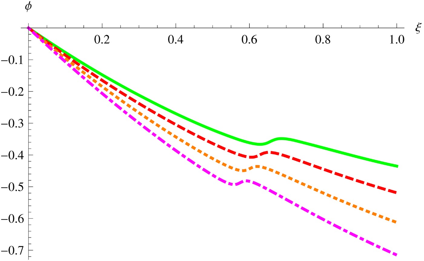
Fig. 6. (Color online) Dependence of longitudinal phase delay ϕ on the magnetic field as a function of dimensionless distance of propagation ξ in a collisionless magnetoplasma with relativistic nonlinearity for b = 0. The parameters used here are: ![]() . Solid curve correspond to when
. Solid curve correspond to when ![]() , dashed curve correspond to when
, dashed curve correspond to when ![]() and dotted curve correspond to when
and dotted curve correspond to when ![]() , dotdashed curve correspond to when
, dotdashed curve correspond to when ![]() .
.

Fig. 7. (Color online) Dependence of longitudinal phase delay ϕ on the magnetic field as a function of dimensionless distance of propagation ξ in a collisionless magnetoplasma with relativistic nonlinearity for b = 1. The parameters usedhere are: ![]() . Solid curve correspond to when
. Solid curve correspond to when ![]() , dashed curve correspond to when
, dashed curve correspond to when ![]() and dotted curve correspond to when
and dotted curve correspond to when ![]() , dotdashed curve correspond to when
, dotdashed curve correspond to when ![]() .
.
In self-trapped mode, we put d 2a +/dz 2 = 0 in Eq. (19) to highlight the features as how decentred parameter, b determines the behaviour of laser beam in magnetoplasma. Figure 8 depicts the dependence of equilibrium radii R as a function of A(=α |A′0|2) for three values of b. For low values of b, the present investigation predicts higher values of equilibrium radii with faster monotonic fall with increase in intensity. However, increase in values of b results in lower values of equilibrium radii as well as weaker dependence on intensity. The behaviour is quite similar to the earlier prediction based on variational approach (Anderson & Bonnedal, Reference Chessa, Mora and Antonsen1979; Anderson, Reference Anderson1978).

Fig. 8. (Color online) Plot of equilibrium beam width R as intensity parameter ![]() for different value of decentred parameter (b). The parameters used here are:
for different value of decentred parameter (b). The parameters used here are: ![]() . Solid curve correspond to when b = 0, dashed curve corresponds to b = 0.5 and dotted curve correspond to b = 1.
. Solid curve correspond to when b = 0, dashed curve corresponds to b = 0.5 and dotted curve correspond to b = 1.
5. CONCLUSIONS
In the present investigation, we have studied self-focusing and self-phase modulation of laser beam in relativistic magnetoplasma. Equation for beam width parameter is derived using variational approach. We find that study of cosh-Gaussian beams can be analyzed like Gaussian beam in plasma, but the decentred parameter and absorption coefficient are found to play key role on the nature of self-focusing/defocusing of the beam.
ACKNOWLEDGMENT
R. K. and R. M. gratefully acknowledge for financial support by Guru Nanak Dev University, Amritsar India.


