


1. INTRODUCTION
Large-scale, high intensity laser installations (Cook et al., Reference Cook, Kozioziemski, Nikroo, Wilkens, Bhandarkar, Forsman, Haan, Hoppe, Huang, Mapoles, Moody, Sater, Seugling, Takagi and Xu2008; Blanchot et al., Reference Blanchot, Bignon, Coïc, Cotel, Couturier, Deschaseaux and Forget2006; Delettrez et al., Reference Glezos and Raptis2005; Danson et al., Reference Danson2005; Dunne, Reference Gurevich, Lukyanov, Zybin, Roussel-Dupré, Kortshagen and Tsendin2006; Miyanaga et al., Reference Synge2003; Neumayer et al., Reference Neumayer, Bock, Borneis, Brambrink, Brand, Caird, Campbell, Gaul, Goette, Haefner, Hahn, Heuck, Hoffmann, Javorkova, Kluge, Kuel, Kunzer, Merz, Onkels, Perry, Reemts, Roth, Samek, Schaumann, Schrader, Seelig, Tauschitz, Thiel, Ursescu, Wiewior, Wittrock and Zielbauer2005) can achieve highly relativistic intensities and generate extremely high currents of relativistic electrons in interaction with solid targets. An accurate description of the transport of such high currents of relativistic electrons in dense matter is an important issue for many applications including the fast ignition of thermonuclear fusion targets, radiography of dense opaque objects, cancer therapy, lithography, etc. (Borghesi et al., Reference Borghesi, Campbell, Schiavi, illi, Galimberti, Gizzi, Mackinnon, Snavely, Patel, Hatchett, Key and Nazarov2002; Glezos & Raptis, Reference Honrubia, Antonicci and Moreno1996; Mangles et al., Reference Stewart2006). Recent proposed schemes for ignition also rely on pre-assembled overdense targets (Holmlid et al., Reference Holmlid, Hora, Miley and Yang2009) and might face such regimes.
The complexity of this problem comes from the fact that the collective and collisional processes are operating in the same time and spatial scales and they require a kinetic description of particles in a very broad energy domain ranging from thermal electrons of a few tens or hundred eV of the main plasma to several tens of MeV of the beam electrons. The dominant physical processes include the collisions of beam electrons with the electrons and ions of plasma, the electron-ion and electron-electron collisions of plasma particles, production of secondary energetic electrons in head-on electron-electron collisions, generation of self-consistent electric and magnetic fields, return currents, and plasma heating. There is a necessity to describe correctly both the energy deposition of beam electrons and their transport from the injection to the energy deposition region.
A very large difference in energies and densities between the electron beam and the plasma electrons are revealed in the time and spatial scales of the collective and collisional processes, that makes it difficult to describe all physical processes within the same kinetic equation. It was suggested to separate the plasma and beam electrons and to consider them as two different populations. A theoretical approach that is currently implemented is based on the hybrid model where the plasma electrons are described in the fluid approximation, while the beam electrons are treated kinetically (Bell et al., Reference Bell, Davies, Guerin and Ruhl1997; Davies, Reference Dubroca and Feugeas2003; Honrubia et al., Reference Mangles, Walton, Najmudin, Dangor, Krushelnick, Malka, Manclossi, Lopes, Carias, Mendes and Dorchies2004). While this approach has shown its capability to describe the major effects such as the collisional slowing down of beam electrons and the return current generation along with the self-consistent electric and magnetic fields, certain physical effects are left out of the frames of this model. In particular, the plasma electron distribution function is supposed to be close to the Maxwellian function and therefore the nonlocal effects in the plasma electric and thermal conductivities are neglected. Moreover, production of secondary fast electrons created in the head-on collisions of the beam and plasma electrons is discarded. A more advanced model of the fast electron transport would be necessary in order to evaluate the domain of validity of the hybrid model and to extend it to higher current densities, higher beam electron energies, and higher plasma densities.
The relativistic extension of the integro-differential Fokker-Planck-Landau kinetic equation (Beliaev & Budker, Reference Beliaev and Budker1956) or simplified techniques (Braams & Karney, Reference Braams and Karney1987; Robiche & Rax, Reference Robiche and Rax2004; Karney & Fisch, Reference Gurevich, Zybin and Roussel-Dupré1985; Bell et al., Reference Bell, Robinson, Sherlock, Kingham and Rozmus2006), have been proposed to incorporate the relativistic effects in the collisional process in the pitch-angle description. Several studies (Robinson et al., 2008; Sherlock et al., Reference Sherlock, Bell, Kingham, Robinson and Bingham2007) have been undertaken recently based on an electron kinetic code KALOS (Bell et al., Reference Bell, Robinson, Sherlock, Kingham and Rozmus2006) to investigate issues related to the fast electron beam energy deposition in fusion targets. There the pitch-angle electron collisions and the self-consistent fields are described relativistically, however the effect of secondary electron production, including both relativistic effects and large momentum transfers, was neglected. The objective of this paper is to consider in detail this latter process and to evaluate its importance, from a theoretical point of view, and from the point of view of numerical treatment of the kinetic equation.
The problem of secondary electron production has been addressed (Gurevich et al., Reference Gurevich, Zybin and Roussel-Dupré1998a, Reference Lefebvre, Cochet, Fritzler, Malka, Aléonard, Chemin, Darbon, Disdier, Faure, Fedotoff, Landoas, Malka, Méot, Morel, Rabec, Gloahec, Rouyer, Rubbelynck, Tikhonchuk, Wrobel, Audebert and Rousseaux1998b) that consider the effect of cosmic rays on the thunderstorm discharges in the Earth atmosphere. A kinetic modeling technique based on the relativistic Boltzmann equation, have been setup to describe large angle scattering processes and production of secondary electrons, that is often called the ionization process. Such specific models have also been derived for gas discharges, runaway breakdown (Gurevich et al., Reference Gurevich, Zybin and Roussel-Dupré1998a), and Tokamak disruptions (Eriksson & Helander, Reference Eriksson and Helander2003; Eriksson et al., 2004). However, these models describe the background electrons as a cold (Gurevich et al., Reference Gurevich, Zybin and Roussel-Dupré1998a) or a warm fluid (Eriksson & Helander, Reference Gurevich and Zybin2003), and consider them as a potential source of secondary electrons. The effect of the energy deposition in plasma was not considered there, whereas it is an important issue for the transport problem. A non-Maxwellian distribution function of plasma electrons could be responsible for the modification of the electric conductivity, return current, and other important effects (Sherlock et al., 2007).
The numerical realization of the relativistic collisional operator has been developed for the collisional particle-in-cell (PIC) or Monte Carlo (MC) codes (Sentoku & Kemp, Reference Sentoku and Kemp2008; Eriksson & Helander, Reference Gurevich and Zybin2003). However, independently of the domain of application, laser interaction with dense matter or a Tokamak plasma, the implementation cost of probabilistic methods into the kinetic models may be too high due to a large number of particles/macroparticles needed to maintain an acceptable low level of statistical fluctuations. Even PIC codes using weighted macroparticules (Sentoku & Kemp, Reference Sentoku and Kemp2008) heavily rely on the small angle scattering to do so. This has lead authors (Eriksson & Helander, Reference Gurevich and Zybin2003) to derive a more specific model that incorporates specifically the production of secondary electrons.
The deterministic numerical methods (Symbalisty et al., Reference Symbalisty, Roussel, Dupré and Yukhimuk1998) could be better suited for description of the large angle scattering effects, because they are by nature less dependent on the density, and temperature conditions. As we will show in this paper, the plasma heating process, which is due to small angle collisions, is on the same order, with a logarithmic accuracy, as the production of secondary electrons, due to large angle collisions. This rather general result will be illustrated here for simple distribution functions for the bulk and beam electrons.
A collisional interaction between the electrons in very different energy scales (from eV to MeV) justifies a need for two populations of electrons: the beam (fast) and the bulk (thermal) particles. However, a direct separation of two populations in the energy or momentum space cannot be efficient, since the bulk electron distribution function may have a long tail, and the fast particle distribution function may have an extension down to the fastest thermal particles. One has to allow for the particle to be transferred from one population to another. In this paper, we propose a model based on the electron kinetic equation, that separates the electrons in two populations operating in two different energy scales. The model is derived by using a procedure based on an operator decomposition technique, where the collision operators are interpreted in a systematic manner. This model respects the particle number, momentum and energy conservations, and introduces an artificial screening parameter in the cross sections, depending on the bulk electron temperature. A reasonable choice for this parameter is fundamental to maintain an acceptable number of particles in each population. Thus, a numerical validation of the present model is necessary to find a compromise for this parameter, and to gain confidence in the results.
The present article is structured as follows. In Section 2, the electron collision processes are described, a two population model is proposed, and its design principles are discussed. In Section 3, the collision invariant preserving property of the procedure is highlighted. Then, basic properties of the model are illustrated on a simple beam-plasma configuration in Section 4. Finally, a reduced model suitable for numerical computations is presented in Section 5. A quantitative analysis is performed for the case of a mono-energetic electron beam propagation in a warm plasma. The importance of large angle scattering for the energy deposition and angular scattering of the beam is demonstrated.
2. RELATIVISTIC MODEL OF ELECTRON KINETICS
2.1. Collision Processes of Importance for Plasma Physics
Let us consider a plasma made of electrons and immobile ionsFootnote 1 of a charge Ze and a density n i. The electrons are described by a relativistic kinetic equation
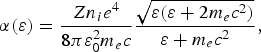
Here, q e = −e is the charge of electron, the velocity and momentum v = p/m eγ are related by the relativistic factor ![]() , c is the speed of light, and m e is the mass of electron. The electric and magnetic fields are described by the Maxwell's equations, where the electric charge and current densities, ρ = e(Zn i − n e) and j are defined by the electron distribution function: n e(t, x) = ∫f e(t, x, p)d p and j(t, x) = q e ∫ f e(t, x, p)vd p. In what follows, we concentrate our discussion on the collisional effects leaving apart the convective terms in the left-hand side of Eq. (1). Our main objective is to separate this kinetic equation into the fast and slow components and to describe the coupling between them.
, c is the speed of light, and m e is the mass of electron. The electric and magnetic fields are described by the Maxwell's equations, where the electric charge and current densities, ρ = e(Zn i − n e) and j are defined by the electron distribution function: n e(t, x) = ∫f e(t, x, p)d p and j(t, x) = q e ∫ f e(t, x, p)vd p. In what follows, we concentrate our discussion on the collisional effects leaving apart the convective terms in the left-hand side of Eq. (1). Our main objective is to separate this kinetic equation into the fast and slow components and to describe the coupling between them.
The standard approach in the physics of Coulomb collisions consists in developing the collision integrals in series assuming a small momentum transfer in each collision. That reduces the general Boltzmann-like collision integral in the Landau-Fokker-Planck differential form containing the friction and diffusion terms in the phase space:
In the non-relativistic limit and neglecting small ion mass corrections, m e/m i ≪ 1, the electron-ion collision integral has only a diffusion term, F Di ≃ 0, that is
where Φ(u) = (|u|2I − u ⊗ u)/|u|3 is the tensor describing the pitch angle scattering, u = v − v′ is the relative velocity, I is the unitary matrix, and lnΛ = ln(Δp max/Δp min) is the Coulomb logarithm, with Δp max ~ p being the maximum momentum transfer in a collision between particles, Δp min ≃ ħ/λD is the minimum momentum transfer at the Debye cut-off, λD, and ħ is the Planck constant. The expressions for the electron-electron friction force and the diffusion coefficient, in the relativistic case, are as follows
In plasmas with highly charged ions, Z ≫ 1, the electron-ion collisions dominate the diffusion, while the friction is related to the electron-electron collisions.
An usual approximation of classical plasmas, where ln Λ ≫ 1, justifies the possibility to neglect the head-on collisions, which makes usually a small contribution on the order of 1/ln Λ. However, this statement of unimportance of large angle scattering events is not general, and there are conditions where the hard collisions could produce qualitatively new effects that do not exist in the Landau-Fokker-Planck approximation. One well-known example is the ionization of atoms or molecules by free electrons in partially-ionized plasmas. Another example is the electron-ion collisions in a strong laser field. The hard collisions dominate the electron heating rate if the electron quiver velocity is larger than the electron thermal velocity multiplied by the Coulomb logarithm (Brantov et al., Reference Brantov, Rozmus, Sydora, Capjack, Bychenkov and Tikhonchuk2003).
In what follows, we are considering a problem of an electron beam propagation through plasma. The characteristic beam electron energy, ɛb, is supposed to be much larger than the mean energy, k BT e, of the bulk electron population. In that case, the hard collisions of the beam and bulk electrons, similarly as in the ionization process, produce energetic electrons, and thus increase the fast electron population. Moreover, the collisions of beam and bulk electrons at small angles produce a fast electron tail in the bulk of electron distribution, which might affect the transport coefficients in such a plasma.
We develop a system of kinetic equations for the beam (fast) electrons described by the distribution function f b, and the bulk (thermal) electrons described by the distribution function f th, assuming that ɛb ≫ k BT e and that density of beam is small, n b ≪ n e. We just suppose that the beam electrons could be relativistic, while the plasma electrons are non-relativistic, k BT e ≪ m ec 2.
2.2. Kinetic Equations for Two Electron Populations
The master equation that incorporates the hard collision processes is the relativistic Boltzmann equation (De Groot et al., Reference Eriksson, Helander, Andersson, Anderson and Lisak1980; Stewart 1971; Synge, 1957)
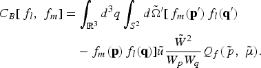
The notations for the momenta p, q, and energies W p, W q are applied to the outgoing particles, that is, after a collision event, whereas the momenta p′, q′, and energies W p′, W q′ refer to the ingoing particles, that is, before the same collision event. The conservation of the momentum and the energy in the collision implies that p + q = p′ + q′ and W p + W q = W p′ + W q′. The quantities marked with tilde (respectively without tilde) refer to quantities in the center of mass frame (respectively, in the laboratory frame) for a collision event, except for the scattering angle in the center of mass frame, denoted by θ. In particular, ![]() is the energy of colliding particles in the center of mass,
is the energy of colliding particles in the center of mass, ![]() is the cosine of the interaction angle.
is the cosine of the interaction angle. ![]() is the relative velocity.
is the relative velocity. ![]() is the Møller velocity, and Q is the total relativistic Rutherford cross section (7), that takes into account both relativistic and spin (including Pauli statistical principle) effects
is the Møller velocity, and Q is the total relativistic Rutherford cross section (7), that takes into account both relativistic and spin (including Pauli statistical principle) effects
where ![]() and the momentum-dependent functions are
and the momentum-dependent functions are ![]() ,
, ![]() ,
, ![]() .
.
The stiffness of the Boltmann operator is due to the long range Coulomb interaction. The complexity of its tensorial form, acting on the general distribution function f (gathering both thermal and fast particules), makes a numerical treatment very difficult. We develop a simplification procedure of the Boltzmann operator, that captures the essential processes and associated collision frequencies with good accuracy. This procedure is relying on appropriate assumptions that respect the original collision invariants.
The first step is folding of the total cross section (7) Q → Q f. Owing to the fact that electrons have to be considered identical, the cross section can be folded, that is, the electrons in the outgoing channel can be exchanged, and the singularities be concentrated at small angles. This step is necessary for development of the small angle scattering approach, and for derivation of the Landau type formulation presented in Eqs. (16)–(18).
As a second step, an intermediate—in momentum exchange—screening is introduced in the Rutherford cross-section, that makes it possible to discriminate between the smaller and larger angles (equivalently energy exchanges) for scattering, and thus to introduce a cut-off volume in the momentum space. This strategy is equivalent to the decomposition, at a finer level though, of the screened Coulomb potential V(r) (Cohen-Tannoudji et al., Reference Cohen-Tannoudji, Diu and Lalöe1986)
![V\lpar r\rpar = \left[\displaystyle{{e^{-r/\lambda_D} \over r}} - {\open S}\lpar r\rpar \right]_{``smaller\; angles''} + \left[{\open S}\lpar r\rpar \right]_{``larger\; angles''}\comma \;](https://static.cambridge.org/binary/version/id/urn:cambridge.org:id:binary:20151021110251605-0723:S0263034610000042_eqnU1.gif?pub-status=live)
where ![]() is a smoothing function, which introduces an upper screening, and
is a smoothing function, which introduces an upper screening, and ![]() .
.
This Debye-like screening procedure of the Coulomb singularity allows a re-interpretation of the above bracketed collisional processes. A rough, but sufficient condition, for such an interpretation to be safe, reads (Gurevich et al., Reference Gurevich, Zybin and Roussel-Dupré1998a)
which reduces, for the model, the admissible configurations of the plasma. Here the subscripts b′ and th′ refer, respectively, to the beam and thermal plasma populations. After a standard folding procedure of the cross-section of like particle collisions, it is decomposed, based on the intermediate screening, in two—or more than two—daughter cross sections. Each of these sub-cross sections is interpreted as a specific collisional process—either the smaller or larger angle scattering—which offers the possibility for a discrimination between two sets of particles, based on the momentum cut-off, and leads to the subsequent operators. Such a decomposition preserves a generality of the description, but is not unique. The positivity of the daughter cross sections is preserved during the decomposition. In the limit defined by the angle ![]() , the smaller angle scattering processes are selected. The larger angle ones shall be discarded by a Fokker-Planck-Landau procedure. On the other hand, the uppper cut-off θa > θD, above the Debye screening, defines the frontier between the smaller and larger scattering angles, and could be chosen such as to respect a robustness criteria, that is, crucial for the numerical implementation of the model. The possiblity remains open to select an anisotropic cut-off in the momentum phase space.
, the smaller angle scattering processes are selected. The larger angle ones shall be discarded by a Fokker-Planck-Landau procedure. On the other hand, the uppper cut-off θa > θD, above the Debye screening, defines the frontier between the smaller and larger scattering angles, and could be chosen such as to respect a robustness criteria, that is, crucial for the numerical implementation of the model. The possiblity remains open to select an anisotropic cut-off in the momentum phase space.
The folded, screened cross section, reads ![]() , where a possible choice for the daughter cross sections is as follows
, where a possible choice for the daughter cross sections is as follows
![Q_f^{\lpar sa\rpar } \lpar \tilde{\,p}\comma \; \tilde{\mu}\rpar = {2Q_0 A\lpar \tilde{\,p}\rpar \over \left(\sin^2 \lpar \theta/2\rpar + \left[\textstyle{{\theta_D \over 2}}\right]^2\right)^2} - {2Q_0 A\lpar \tilde{\,p}\rpar \over \left(\sin^2 \lpar \theta/2\rpar + \left[\textstyle{{\theta_a \over 2}}\right]^2\right)^2}\comma \;](https://static.cambridge.org/binary/version/id/urn:cambridge.org:id:binary:20151021110251605-0723:S0263034610000042_eqn8.gif?pub-status=live)
![\eqalign{Q_f^{\lpar la\rpar } \lpar \tilde{\,p}\comma \; \tilde{\mu}\rpar &= {2Q_0 A\lpar \tilde{\,p}\rpar \over \left(\sin^2 \lpar \theta/2\rpar + \left[\textstyle{{\theta_a \over 2}}\right]^2\right)^2} \cr &\quad - {2Q_0 B\lpar \tilde{\,p}\rpar \over \sin^2 \lpar \theta/2\rpar + \left[\textstyle{{\theta_a \over 2}}\right]^2} + Q_0 C\lpar \tilde{\,p}\rpar . \cr}](https://static.cambridge.org/binary/version/id/urn:cambridge.org:id:binary:20151021110251605-0723:S0263034610000042_eqn9.gif?pub-status=live)
Both functions are positively defined. The inclusion of screening terms in the nonlogarithmic terms is allowed because the relevent range for the parameter θa satisfies the multi-scale criteria θD ≪ θa ≪ 1, which involves ![]() . It does not affect the accuracy of the cross section, since the contributing, singular part remains physically screened. Rather than the decomposition (8)–(9), we prefer the screening and decomposition such as
. It does not affect the accuracy of the cross section, since the contributing, singular part remains physically screened. Rather than the decomposition (8)–(9), we prefer the screening and decomposition such as
![\eqalign{Q_f^{\lpar sa\rpar } \lpar \tilde{\,p}\comma \; \tilde{\mu}\rpar &= {2Q_0 A\lpar \tilde{\,p}\rpar \over \left(\sin^2 \lpar \theta/2\rpar + \left[\textstyle{{\theta_D \over 2}}\right]^2\right)^2}\cr &\quad - {2Q_0 A\lpar \tilde{\,p}\rpar \cos^2 \left(\textstyle{{\theta \over 2}}\right)\over \left(1 + \left[\textstyle{{\theta_a \over 2}}\right]^2\right)\left(\sin^2 \lpar \theta/2\rpar + \left[\textstyle{{\theta_a \over 2}}\right]^2\right)^2}\comma \; \cr}](https://static.cambridge.org/binary/version/id/urn:cambridge.org:id:binary:20151021110251605-0723:S0263034610000042_eqn10.gif?pub-status=live)
![\eqalign{Q_f^{\lpar la\rpar } \lpar \tilde{\,p}\comma \; \tilde{\mu}\rpar &= {2Q_0 A\lpar \tilde{\,p}\rpar \cos^2 \left(\textstyle{{\theta \over 2}}\right)\over \left(1 + \left[\textstyle{{\theta_a \over 2}}\right]^2\right)\left(\sin^2 \lpar \theta/2\rpar + \left[\textstyle{{\theta_a \over 2}}\right]^2\right)^2} \cr &\quad - \left[{\cos^2 \left(\textstyle{{\theta_a \over 2}}\right)\over 1 + \left[\textstyle{{\theta_a \over 2}}\right]^2}\right]{2Q_0 B\lpar \tilde{\,p}\rpar \over \left(\sin^2 \lpar \theta/2\rpar + \left[\textstyle{{\theta_a \over 2}}\right]^2\right)} + Q_0 C\lpar \tilde{\,p}\rpar . \cr}](https://static.cambridge.org/binary/version/id/urn:cambridge.org:id:binary:20151021110251605-0723:S0263034610000042_eqn11.gif?pub-status=live)
These daughter cross sections are positive. This form allows us to simplify forthcoming analytical computations and to postpone crucial hypothesis at the end of the computation.
The distinction between thermal f thθa and beam f bθa distribution functions is the consequence of the discrimination of the collisional processes. As a matter of fact, the two populations present two different resolutions for the phase-space discretization. In the remainder of the paper, we drop the superscripts θa on the distribution functions.
The processes associated with each of the two energy scales are listed in Table 1. The two electron populations, thermal and fast, are allowed to share energy ranges, provided distinct energy exchange scales can be identified among the collision processes at stake. This leads to a simplification of the Bolzmann operator to a set of bilinear operators. The modeling choice for these operators and the attribution procedure to each of the populations, are also given in Table 1.
Table 1. List of collisional processes considered for the beam and plasma electrons

Concerning the thermal population, only pitch angle scattering between the thermal particles is taken into account (process ST(sa)). The large angle scattering of the thermal particle (process ST(la)) is neglected assuming 1/ln Λ as a small parameter. The collisions of the thermal particles with the beam particles give raise to three processes. The small angle scattering (H) increases the energy of the thermal particle, while leaving it in its own population. The large angle scattering (IO) has two manifestations: the thermal particle gains energy and joins the beam population (IO+) — this is the ionization term — and, at the same time, the thermal population looses this particle (IO−).
Concerning the beam population, the process SD(sa) is identified as the small angle scattering on the thermal particles. It is the standard Fokker-Planck-Landau process producing the diffusion and friction of the beam in the phase space. The process SD(la) can be interpreted as large angle scattering of beam particles on the thermal particles, where particles of each population are maintained, in the outgoing channel (at the end of the collision process), in their original populations. This appears paradoxal, since the large angle scattering statement should be responsible for a thermal particle to become member of the beam population. We solve this by choosing a Fokker-Planck approach (see Section 3) for the process SD(la), that maintains the collision invariants of the bilinear Boltzmann form. Doing so, makes the large energy exchanges discarded for thermal particles, as non-physical in this process. This is possible because we considered folded cross sections around small angles, and thus all scattering angles are gathered (considering the forward peakness of the Coulomb cross section) around zero. This Fokker-Planck treatment is valid for the beam particles as well, since the large energy exchanges can still be considered small with respect to the variation of the beam distribution function. Finally, all collisions between the beam particles are neglected because of a relatively small number of beam electrons.
The final model, that presents two energy exchange scales, reduces to
where the explicit forms of the collision operators are presented in Eqs. (14)–(18). In particular, the operators that describe hard collisions, where the two populations exchange particles, read
where the delta function accounts for the property of energy conservation for a collision between a fast and a thermal particle, in the center of mass frame. The last two forms on the right-hand side of Eq. (12) are merged in C SD[f b, f th] = C SD (sa) [f b, f th] + C SD (la) [f b, f th]. The other processes can be described in the pitch angle limit
The friction force F De and diffusion coefficient De are given in Eqs. (4) and (5), because only small angle deviations in the non-relativistic regime are considered, with a logarithmic accuracy, for the scattering of thermal particles.
Finally, the bilinear forms C H[f th, f b] (Heating, with the cross section Q f(sa)), and C SD[f b, f th] (slowing down, with the cross section Q f), of the Bethe type, are derived following the Landau method. The resulting expressions for the coefficients F D[f] and D[f] are given in Eqs. (20)–(21) and (27)–(29). They are respecting the collision invariants — the conservation of the total mass, momentum, and energy — for the complete distribution function f th + f b, for the model (12)–(13). The derivation presented in the next section is based on a decomposition of the collision operator in moments of the cross section. Compared to the original Landau derivation, the present approach differs only in non-logarithmic terms, but has the advantage of exactly preserving the collision invariants of the model, thus contributing to gain a confidence into it.
3. AN INVARIANT PRESERVING FOKKER-PLANCK PROCEDURE
We propose here a Fokker-Planck procedure of derivation of the model (12) – (13) from the original Boltzmann operator (7). Its particularity lies in the preservation of the collision invariants — total mass, momentum and energy — for each process of the model, independently. The derivation of Fokker-Planck type operators starts from the weak form of the Boltzmann operator, operating on a arbitrary, forward-peaked folded cross section Q f. Let us consider an arbitrary smooth test function ![]() , and calculate the following integral
, and calculate the following integral
The right-hand side of this equation can be rewritten, exchanging the incoming {p′, q′} and outgoing particles {p, q}, as
Then a Taylor expansion is performed on the functions ![]() and f, assuming small angle deviations, Δp ≪ p (small energy exchanges), and using the momentum conservation p′ + q′ = p + q
and f, assuming small angle deviations, Δp ≪ p (small energy exchanges), and using the momentum conservation p′ + q′ = p + q
Only the terms being less than first order are retained, in these developments. Then we obtain the differential Landau form of the operator
where the drag force F D and the matrix D are
These coefficients only depend on the matrix 〈ΔpΔp〉, whose components are defined by
where the integration is conducted in the center of mass frame over the polar and azimuthal angles ![]() and
and ![]() . If two distinct populations, f l and f m are introduced (l and m referring either to the thermal or beam population), the following Boltzmann bilinear form is considered,
. If two distinct populations, f l and f m are introduced (l and m referring either to the thermal or beam population), the following Boltzmann bilinear form is considered,
A first order Taylor expansion leads to the corresponding Landau bilinear form
The coefficients of this operator are written explicitly by using a decomposition with moments of the cross section. This avoids logarithmic approximations of this cross section Q f, which remains the same for the Fokker-Planck and the Boltzmann operators. In the next section, we develop this procedure and justify formally that the Landau operator (19) (respectively the Landau bilinear form (24)) reproduces the conservation properties of the initial Boltzmann equation (6) (respectively the Boltzmann bilinear forms (23)).
3.1. A Fokker-Planck Procedure Based on Moment Decomposition
Let the cross section Q f be arbitrary in this section, though forward-peaked. The analysis we propose here is based on the decomposition of the momentum exchange Δp = Δp ||n + Δp⊥ in one parallel and two perpendicular components, with respect to the velocity V = V n of the center of mass frame in the laboratory frame. If a Taylor expansion is performed on the weak form of Botzmann Eq. (6), with infinite order, the so-obtained operator C[f, f](Q f) involves the coefficients
where the subscripts ⊥1 and ⊥2 refer to each perpendicular directions, and the brackets are defined by the Eq. (22).
The parallel component does not depend on the azimuthal angle ![]() . Then if k + l is odd, the coefficient
. Then if k + l is odd, the coefficient ![]() is equal to zero, after integration in
is equal to zero, after integration in ![]() . In the case where k + l is even, we obtain
. In the case where k + l is even, we obtain
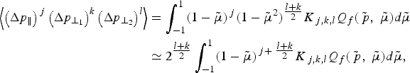
where the coefficients K j,k,l only depend on the variables ![]() , V, Wp, Wq, but not on the variable
, V, Wp, Wq, but not on the variable ![]() . At this point we have made the logarithmic approximation
. At this point we have made the logarithmic approximation ![]() for the coefficient
for the coefficient ![]() , in the case k + l is even, assuming that the dominant contribution comes from the small angles, because of the divergence of the cross section. This allows to rearrange formally the operator as the infinite sum
, in the case k + l is even, assuming that the dominant contribution comes from the small angles, because of the divergence of the cross section. This allows to rearrange formally the operator as the infinite sum

whatever the expression of the cross section is. In this decomposition, the contribution of the m th moment of the cross section ![]() is assigned to the formal operator C (m)(Q f). Since this decomposition does not assume the explicit knowledge of the cross section, all the properties of the operator C(Q f) hold for each operator C (m)(Q f). In particular, dropping terms with m > 1, the collision invariants are preserved for the operator C (1)(Q f). This procedure remains valid when bilinear forms are considered for two distinct populations. Then we obtain the conservation properties on these bilinear forms
is assigned to the formal operator C (m)(Q f). Since this decomposition does not assume the explicit knowledge of the cross section, all the properties of the operator C(Q f) hold for each operator C (m)(Q f). In particular, dropping terms with m > 1, the collision invariants are preserved for the operator C (1)(Q f). This procedure remains valid when bilinear forms are considered for two distinct populations. Then we obtain the conservation properties on these bilinear forms
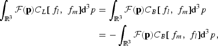
where ![]() can be either p, or W p. Moreover the only equilibrium states of this operator are the Maxwellian distribution functions f l and f m whose temperature and mean velocity are the same. These conservation properties can be rigourously proved for the operators (16)–(17), with the explicit expressions of the Fokker-Planck components (27)–(29), given in the next section. The energy conservation will be illustrated in the case of a model issued from (Gurevich et al., Reference Gurevich, Zybin and Roussel-Dupré1998a), that has been modified following this procedure, in Section 4.1.
can be either p, or W p. Moreover the only equilibrium states of this operator are the Maxwellian distribution functions f l and f m whose temperature and mean velocity are the same. These conservation properties can be rigourously proved for the operators (16)–(17), with the explicit expressions of the Fokker-Planck components (27)–(29), given in the next section. The energy conservation will be illustrated in the case of a model issued from (Gurevich et al., Reference Gurevich, Zybin and Roussel-Dupré1998a), that has been modified following this procedure, in Section 4.1.
This approach only differs from the original Landau-Fokker-Planck development in non-logarithmic terms. However, these additional non-logarithmic contribution prove to be essential to maintain the correct conservation properties (26) all through the model derivation.
3.2. Explicit expression of the Fokker-Planck coefficients
In this section, we choose the cross section Q f, defined by the sum of Eqs. (10) and (11), and derive the Fokker-Planck coefficients from the above presented Fokker-Planck procedure. The cross section shows a singularity at ![]() , that corresponds to small angle scattering. Then the operator C (1)(Q f) contains both logarithmic and non-logarithmic terms; the non-logarithmic contribution being located inside the cross section. The other operators C (m)(Q f), m > 1, only contain non-logarithmic terms, and are dropped in the rest of the paper.
, that corresponds to small angle scattering. Then the operator C (1)(Q f) contains both logarithmic and non-logarithmic terms; the non-logarithmic contribution being located inside the cross section. The other operators C (m)(Q f), m > 1, only contain non-logarithmic terms, and are dropped in the rest of the paper.
The coefficient 〈ΔpΔp〉 is no more a pure diffusion matrix if the Landau derivation of Section 3.1 is applied. In this context, the quantities 〈ΔpΔp〉 and ∇q · 〈ΔpΔp〉 are written as
where the matrix M is defined as
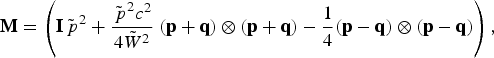
and thus
With this approximation, the coefficients satisfy the relation −∇q·〈ΔpΔp〉 = 2〈Δp〉 − ∇p·〈ΔpΔp〉. Therefore, we obtain the equivalence between the Landau operator of Eq. (19) and the Fokker-Planck form
The equivalence between the Landau and Fokker-Planck forms remains true for the bilinear operators.
3.3. Coulomb Logarithms and Cross Sections
The collision integral C SD describes the scattering of beam on plasma electrons. Its Coulomb logarithm is defined with the Debye cut-off parameter θD. It is contained in the coefficient ![]() . The contribution of the collisions between beam electrons and ions can be directly incorporated, substituting Z → Z + 1.
. The contribution of the collisions between beam electrons and ions can be directly incorporated, substituting Z → Z + 1.
The plasma heating (process H in Table 1) is defined by the energy deposition of fast particles, while they are scattered on small angles on the plasma electrons. The Coulomb logarithm is contained in the coefficient ![]() .
.
The Boltzmann operators that exchange particles (processes IO ± in Table 1), have an integral form that presents a logarithmic singularity. The analogy with the Coulomb logarithm will be illustrated in the case of a beam electron population in Section 4.
4. ENERGY EXCHANGE OF BEAM ELECTRONS IN A COLD PLASMA
4.1. Kinetic Equation for Beam Electrons
Relativistic electron-ion and electron-electron collision operators for a low density electron beam propagating through a cold and dense plasma were derived in (Gurevich et al., Reference Gurevich, Zybin and Roussel-Dupré1998a). It was shown that under the conditions n b ≪ n e and εb ≫ k BT e, they can be presented as a sum of three terms. The first two terms correspond to the small angle collisions (process E in Table 1), and they have a Fokker-Planck differential form (2):
The drag force F D is due to the electron-electron collisions, while the diffusion term D describes the elastic scattering accounts for the electron-electron and electron-ion collisions. If only logarithmic terms are retained
These expressions are similar to Eqs. (4) and (5) in the non-relativistic case, with the same expression for the Coulomb logarithm. In addition, the large angle collisions (process F in Table 1) are responsible for production of secondary high energy electrons. This term, so-called, ionization integral (Gurevich et al., Reference Gurevich, Zybin and Roussel-Dupré1998a), reads
Here, the collision rate, α, the kernel, K, and the Delta function accounting for the energy conservation δE, are defined as
where ɛ′ = m ec 2(γ′ − 1) and ɛ = m ec 2(γ − 1) are the kinetic energies of the incoming and outgoing particles, associated to the Lorentz factors γ′ and γ. The momentum p is written in spherical coordinates in terms of the variables (ɛ, μ, φ). Here the ionization integral (32) involves the cross section ![]() folded around the large angles. It is defined as
folded around the large angles. It is defined as ![]() .
.
The integral (32) does not contain the Coulomb logarithm, contrary to the friction and diffusion terms. However it contains a logarithmic dependence on the low energy limit, and that makes it on the same order as the diffusion and friction terms. This is illustrated in the next section for the case of a mono-energetic electron beam.
4.2. Energy Losses of a Mono-Energetic Electron Beam on a Cold Plasma
Let us consider a mono-energetic electron beam with energy ɛb = m ec 2(γb − 1) propagating in a direction defined by the polar axis z. The beam distribution function writes

The beam energy loss is defined as
The beam energy loss due to pitch-angle collisions with plasma electrons is described by the friction term in Eq. (30), which gives
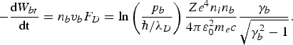
Here, for a background plasma of 0.1 keV, with a density of 1021 cm−3, the minimum kinetic energy ɛmin, related to the momentum ![]() , is of the order of 10 meV.
, is of the order of 10 meV.
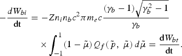
The energy loss due to hard collisions with plasma electrons is obtained from the ionization integral in Eq. (32)
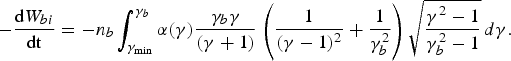
The integral over the energy has a logarithmic divergence at the lower limit γmin ≃ 1, corresponding to small angle collisions.
Further, turning to the Fokker-Planck procedure described in Section 3, we demonstrate an energy conservation property (40), similar to Eq. (26), in the model (with cold plasma) of Gurevich et al. (Reference Gurevich, Zybin and Roussel-Dupré1998a). This model is modified here in two aspects: first, the complete cross sections are retained, and second, the Fokker-Planck derivation procedure described in Section 3 is applied. These modifications lead to the following expression for the energy loss in Eq. (38)
5. REDUCED MODEL FOR FAST ELECTRON DISTRIBUTION FUNCTIONS
5.1. Assumptions Concerning the Electron Distribution Function
In order to simplify the ionization operator (IO), we assume that the thermal electron population, with the density ![]() , has an isotropic energy distribution
, has an isotropic energy distribution
with the normalization ∫1∞ γ(γ2 − 1)1/2F th(γ)dγ = 1. Also, in order to simplify the calculations, we only retain the dominant part of the cross sections, that contains the Coulomb logarithm. The cross sections in the IO can be further simplified, owing to the fact that all the quantities that do not contribute to the logarithmic divergence can be approximated with the assumption of weak dependence with respect to the temperature of the thermal population.
We describe the beam distribution function within the M1 model (Berthon et al., Reference Berthon, Charrier and Dubroca2007; Dubroca & Feugeas Reference Gremillet, Bonnaud and Amiranoff1998; Turpault et al., Reference Turpault2002), that relies on the angular moment closure in the phase space. Its angular dependence is defined from the minimum entropy principle (Levermore, Reference Levermore1996; Minerbo et al., Reference Minerbo1978)
where Ωp is the unit vector in the p momentum direction, ρ0 is a non-negative scalar (ρ0 ≥ 0), and a1 is a three component real valued vector. The functions a1 and ρ0 only depend on the fast electron energy. An important parameter is the anisotropy of beam distribution ![]() , where
, where
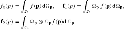
The anisotropy parameter is by construction less or equal than one ![]() . The ansatz (42) ensures the analytical computation of moment f2 as a function of f0 and f1, based on a tabulated Eddington factor (Duclous et al., Reference Duclous, Dubroca and Frank2010), which defines the relation between
. The ansatz (42) ensures the analytical computation of moment f2 as a function of f0 and f1, based on a tabulated Eddington factor (Duclous et al., Reference Duclous, Dubroca and Frank2010), which defines the relation between ![]() and a1.
and a1.
An important feature of the M1 model, consists of the fact that it reproduces exactly both beam-like and isotropic distribution functions. Moreover, the form (42) is convenient for the calculation of the ionization operator that presents a very narrow domain of integration over the angular variable.
Under the assumptions formulated above, the IO operator takes the following form
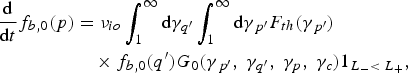
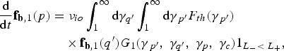
where we have introduced an effective collision frequency νio ≡ e 4n th/4πɛ02m e2c 3, the dimensionless kernels G 0 and G 1, which are regular kernels, 1L −< L + is an indicative function, valued 1, if L − < L +, and 0 otherwise, with ![]() . This indicative function can be narrow, as the energies on the outgoing channel may present a very narrow divergence in angles. However, a fine energy discretization of the thermal population allows to capture this feature. This is an imporatnt aspect of the model. The integrals (43) and (44) depend on the parameter γc that separates the fast and slow electron populations.
. This indicative function can be narrow, as the energies on the outgoing channel may present a very narrow divergence in angles. However, a fine energy discretization of the thermal population allows to capture this feature. This is an imporatnt aspect of the model. The integrals (43) and (44) depend on the parameter γc that separates the fast and slow electron populations.
5.2 Relaxation of a Mono-Energetic Electron Beam in a Thermal Maxwellian Plasma
Let us consider a mono-energetic beam with the distribution function (37) propagating through a homogeneous Maxwellian plasma with a non-relativistic temperature Θth = k BT th/m ec 2 ≪ 1. The finite value of Θth is needed for the calculation of the ionization integral. However, it may be set to zero in the calculations of the slowing down operator (SD), as the particles affected by this process do not move from one population to another. This choice makes it appear an explicit logarithmic divergence of the singularity.
First, we analyse the value of the ionization integral by evaluating the ionization rate, that is, the evolution of the number of beam electrons with time. This provides also with a hint for choosing the separation parameter γc, as it should not lead to a significant leakage of the thermal population.
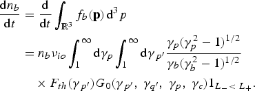
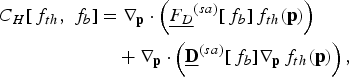
The dependence of the secondary electron production rate on the beam electron energy and on the cut-off parameter is shown in Figure 1 for the representative case of a 5 keV thermal plasma. The ionization rate presents a strong dependence with respect to γc if the cut-off energy is chosen very close to the thermal energy of plasma electrons. This dependence becomes weaker as soon as the cut-off energy goes far in the tail of the plasma distribution function. The production of secondary electrons increases also with the energy of fast electrons. Both these effects can be easily understood if one accounts for the fact that, even in the pitch angle scattering event, the secondary electron gains a significant energy. Indeed, assuming the scattering angle θ ≪ 1 and the large energy of the beam electrons, γb ≫ 1, one finds from the energy and momentum conservation relations that the energy of secondary electron is

Fig. 1. (Color online) Production rate (νion b)−1dn b/dt of secondary electrons by a beam electrons propagating in a 5 keV Maxwellian thermal plasma as a function of the beam energy and the energy cut-off parameter. Isolines 1, 100, 500, 1000, 5000 for the production rates are labelled with respective letters (a)–(e).
The secondary electron energy would be 700 keV if the 5 MeV is scattered to a small angle of 10°. Therefore too small energy cut-off corresponds to accounting for the pitch angle scattered electrons as the secondary beam electrons. For this reason, the choice of the cut-off energy is problem dependent. It must be chosen in such a domain where the dependence of the secondary electron production with respect to the cut-off energy is weak. Figure 1 proves the existence of such a domain for the beam-plasma configuration. Moreover, this figure illustrates two more points: first, the model respects the positivity of G 0, second, the ionization rate profile is peaked for a low energy cut-off.
One can also analyse the relative contribution of the ionization and slowing down mechanisms to the total momentum. In the limit of low plasma temperature and retaining only the logarithmic terms, one finds the following expression for the slowing down rate of the fast electron momentum:
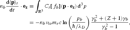
where the Bethe operator (30), with friction and diffusion coefficients (31) was taken into account. The averaged contribution of this process to the total beam momentum is negative.
The contribution to the total beam momentum due to the ionization operator is
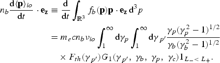
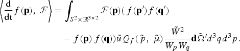
The ratio of the momentum evolution rates (46) over (45) is shown Figure 2. The dependence with respect to the energy cut-off parameter is found to be strong as well, even if the momentum tends to weaken the singularity, compared to Figure 1. Moreover, this ratio exhibits a negative sign, which implies a positive contribution of the secondary electrons into the beam momentum. Large values of this ratio is the signature of the importance of the secondary electron production, under these conditions.

Fig. 2. (Color online) Relative contribution (large over small angle scattering) to the momentum transfer rate of beam particles in a 5 keV Maxwellian thermal plasma as a function of the beam energy and the energy cut-off parameter. Isolines −1, −10, −100, −200, −300, −400 for this ratio are labelled with respective letters (a)–(f).
The conservation of the total momentum in the plasma-beam system implies that the fast electron beam cannot gain energy from plasma. This fact provides another hint for the choice of the cut-off parameter. We are now in position to prescribe a choice for the energy cut-off parameter, that could be defined at an apropriate isosurface in Figure 2, that is, where we can ensure a weak dependence with respect to that parameter.
5.3. Influence of the Energy-Scale Cut-Off Parameter on the Propagation of Oscillations
In Alexandre and Villani (Reference Alexandre and Villani2002), the authors are proposing a sophisticated renormalization procedure upon the non-homogeneous, non-relativistic Boltzmann equation. They show that oscillations are immediately damped by a singular cross section. Conversely, the oscillations, if a cut-off is applied, propagate. The question that arises is: what is the effect of the energy exchange cut-off parameter on the propagation of these oscillations? For instance, one may expect a transfer of these oscillations, at fixed energy, from one population to another. This could be possible because the two populations are allowed to share energy ranges, and also because the Boltzmann gain and loss terms are split between the populations.
6. CONCLUSION
We have shown that the large angle scattering in electron-electron collisions (Shoub Reference Shoub1987), and resulting production of secondary fast electrons (Gurevich et al., Reference Gurevich, Zybin and Roussel-Dupré1998a), is of great importance for the overall dynamics of the electron beam and plasma populations, at relativistic energies. We proposed a robust reduced model to deal with such a mechanism. This model is based on a decomposition of the relativistic Boltzmann collision operator, relying itself on a decomposition over the relativistic Rutherford cross section, instead of a partition of the phase-space between populations, as done usually. This model proposes a natural definition for the thermal and beam populations, according to the collision process they are issued from. The two populations are allowed to share energy ranges in the model. Further quantitative evaluation are foreseen to check the accuracy of the model and quantify the influence of the large angle scattering on the fast electron transport. This can be achieved using Monte-Carlo codes, such as Geant or Penelope. Such comparison could also be profitable contribution for specifications to the HiPER project (J.R. Davies. Fast Electron Transport Calculation for HiPER Benchmarking Collision Routines, Unpublished manuscript). Beyond 10 – 20 MeV beam energies, Bremsstrahlung, density effects, photon production, and creation of electron-positron pairs, should complete this model (Landau & Lifshitz, Reference Robinson, Kingham, Ridgers and Sherlock1973; Lefebvre et al., 1996).


