1. INTRODUCTION
It is well-known that the two-stream instability (TSI) occurs in a conservative system and from this point of view this instability is a general class of reactive instabilities (Hasegawa, Reference Hasegawa1968) that arise due to the interaction between cold electron beams.
TSI is a very common instability in plasma physics (Krall & Trivelpiece, Reference Krall and Trivelpiece1973; Chen, Reference Chen1994). An examination of this instability was investigated by means of a graphical solution of the dispersion relation (Jackson, Reference Jackson1960) and also behavior of opposing streams using numerical simulations (Dawson, Reference Dawson1962). This instability can be generated by two counterstreaming beams, by an energetic particle stream injected into a plasma, or setting a current along the plasma where different species (ions and electrons) can have different drift velocities. In all of the aforementioned examples, the energy of particles can be transferred into the plasma wave excitation. However the TSI has been first studied by a macroscopic moment equation (Haeff, Reference Haeff1949; Pierce, Reference Pierce1948), the complete analytical and numerical investigations have already been detailed in the past decade (Lapenta et al., Reference Lapenta, Markidis, Marocchino and Kaniadakis2007; Dieckmann et al., Reference Dieckmann, Drury and Shukla2006). According to that this instability is relevant to different areas of science, the subject has been constantly studied in a variety of situations (Startsev & Davidson, Reference Startsev and Davidson2006; Silin et al., Reference Silin, Sydora and Sauer2007; Haas et al., Reference Haas, Bret and Shukla2009; Zeba et al., Reference Zeba, Yahia, Shukla and Moslem2012; Startsev et al., Reference Startsev, Kaganovich and Davidson2014).
We know that in the standard assumption of statistical mechanic with Boltzmann-Gibbs (BG) statistics the thermodynamic quantities like energy are “extensive,” meaning that these quantities are proportional to their size V or to the number of particles N. Actually, in the short-range nature of the interactions which hold matter together, this is justified. But if anyone deals with systems with long-range interactions, most prominently gravity and Coulomb electric forces, it is clear that energy is not extensive. This makes hard the life of statistical mechanic.
The necessity of modification of the BG statistics, to achieve a successful model valid for long-range interaction, had been an important challenge among the scientists. A first suitable non-extensive generalization of the BG entropy for statistical equilibrium was reorganized by Renyi (Reference Renyi1955), and Tsallis (Reference Tsallis1988) proposed it subsequently. In Tsallis statistics, correlations between particles play an important role in the fluctuations of the energy whose magnitude is much smaller than that in Boltzmann statistics (Feng & Liu, Reference Feng and Liu2010). Tsallis (Reference Tsallis2002) formulated a non-extensive entropy with an entropic index q. In Tsallis formulation, the standard statistical mechanics is recovered for q → 1 and the super-extensivity, extensivity or sub-extensivity correspond to q < 1, q = 1 or q > 1, respectively.
In the last few years, an increasing attention has been paid to Tsallis statistics. For instance, non-extensive statistics has been used to analyze the subjects such as energy fluctuations (Liyan & Jiulin, Reference Liyan and Jiulin2008) Landau damping of dust acoustic waves (Liu et al., Reference Liu, Qiu and Li2012) and longitudinal oscillation in relativistic plasmas (Liu & Chen, Reference Liu and Chen2011). Furthermore, the effect of the non-extensive parameter q on the nonlinear Landau damping is detailed (Valentini, Reference Valentini2005). The non-extensive statistics is also applied to investigate the instability phenomena, such as the plasma oscillations (Chen & Li, Reference Chen and Li2012) dust ion acoustic instability (Dai et al., Reference Dai, Chen and Li2013) and arbitrary amplitude kinetic Alfven solitons (Liu et al., Reference Liu, Liu and Dai2011).
The particle-in-cell (PIC) method is one of the most popular numerical methods which approximate the plasma by a finite number of particles. The first particle models of an electrostatic plasma were introduced by Buneman (Reference Buneman1959). These models were one-dimensional and did not use a mesh for the calculation of the fields. Dawson at Princeton and Eldridge and Feix in 1962 worked on similar models. The first particle-mesh (PM) algorithm in one dimension was introduced by Burger and in two dimension by Hockney (Hockney & Eastwood, Reference Hockney and Eastwood1988). They used the nearest grid point (NGP) charge model and field interpolation in the PM algorithm. In fact, a PM algorithm is a plasma model that uses finite-size particles or clouds. However, algorithms using such finite-size particles were developed by Birdsall and Langdon (Reference Birdsall and Langdon1985). In recent years, PIC simulations are also used in different areas, such as laser-plasma interaction (Benedetti et al., Reference Benedetti, Londrillo, Petrillo, Serafini, Sgattoni, Tomassini and Turchetti2009) and nonlinear beam plasma interaction (Yoo et al., Reference Yoo, Rhee and Ryu2007).
The first-order weighting in PIC simulation smoothes the density and field fluctuations compared to zero-order weighting or NGP model. Consequently, the PIC weighting scheme produces far less noise than the NGP scheme and tend to reduce nonphysical effects. Therefore, in this paper, we seek estimates for growth of the electrostatic wave driven by TSI by making use of extensive PIC simulations. The electrostatic wave is produced by interpenetration of two counterstreaming electron beams with equal density and opposite bulk velocity in the presence of neutralizing background of the static ions. In the context of the Tsallis statistics, we will assume that the electron beams are described by the non-extensive q-distributions, and so influence of entropic index q on the growth of the TSI will be discussed in the next section.
This paper is organized as five sections. In Section 2, we briefly discuss the initial electron distribution in the context of the Tsallis statistics. In Section 3, the simulation approach and results are presented and the approach is followed to compare the instability generation by initially electron distribution with different q values. In Section 4, the summary and conclusion are presented.
2. INITIALLY ELECTRON DISTRIBUTION AND TSALLIS STATISTICS
As we mentioned previously, the BG statistics may not be proper to describe the long-range natural interactions like a plasma system. The parameter q in the Tsallis statistics represent the degree of non-extensivity of the distribution. This continuous real parameter can be used to adjust the distributions so that distributions can have properties near or far from a Maxwellian distribution. For example, to define the two-streams of energetic beams with particles velocities around the drift velocity, we use the Tsallis statistics with q ≫ 1 and for beams widely spread around the drift velocity, the q ≪ 1 is the best choice (Fig. 1). Therefore, the Tsallis statistics is a generalization of the BG statistics in the same way that Tsallis entropy is a generalization of standard BG entropy. Therefore, in this section we are going to analyze the TSI based on the Tsallis statistics which is very suitable to describe a system with long-range interactions such as a plasma. To do this, we focus our attention to a system described initially by distribution function
 $$\,f\lpar v\rpar = \displaystyle{1 \over 2} \left[\,f_q \lpar v - v_0\comma \; v_{th}\rpar + f_q \lpar v + v_0\comma \; v_{th}\rpar \right]\comma$$
where f q (v) is the so-called Tsallis distribution function define as
 $$\,f_q \lpar v\rpar = \displaystyle{n_0 A_q \over \sqrt{2{\rm \pi}} v_{th}} \left[1 - \lpar q - 1\rpar \displaystyle{v^2 \over 2v_{th}^2} \right]^{\displaystyle{1 \over q - 1}}.$$
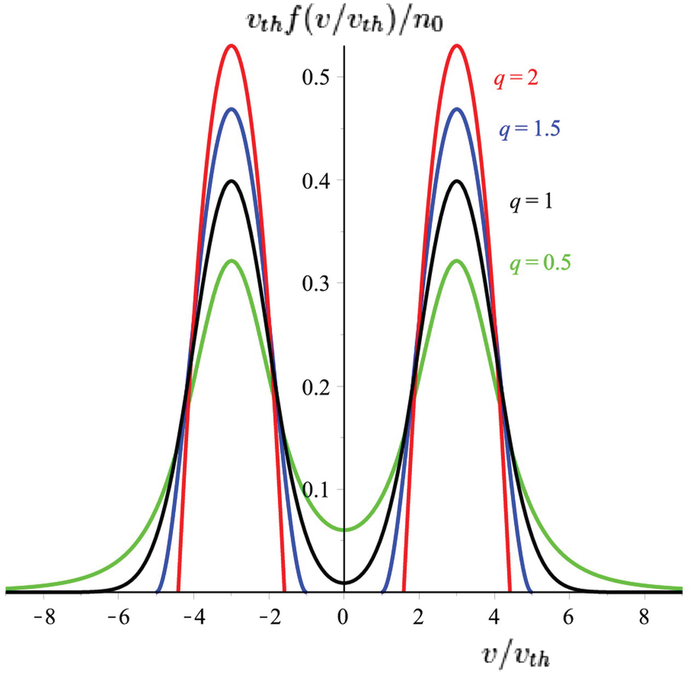
Fig. 1. (Color online) Normalized initial particles distribution function Eq. (1) for various q values and v 0 = 3.
Here  $v_{th} = \sqrt{k_B T \over m} $ is the particle thermal velocity (k B, T, m, are Boltzmann constant, particle temperature, and density, respectively) and the normalization constant A q is given by
 $$\matrix{A_q = \sqrt{1 - q} \left(\displaystyle{\Gamma \lpar {1 \over 1 - q}\rpar \over \Gamma \lpar {1 \over 1 - q} - {1 \over 2}\rpar } \right) &for &0 \lt q \le 1\comma \; \hfill \cr A_q = \displaystyle{1 + q \over 2} \sqrt{q - 1} \left(\displaystyle{\Gamma \lpar {1 \over q - 1} + {1 \over 2}\rpar \over \Gamma \lpar {1 \over q - 1}\rpar } \right) &for &q \ge 1. \hfill}$$
 The distribution function in Eq. (2) for q > 1 restricts the particles velocity to a maximum cut-off value define as  $v_{max} = \sqrt{{2v_{th}^2 \over q - 1}}$. In the limit, q → 1 Tsallis distribution is reduced to the well-known Maxwellian distribution. The system defines as Eq. (1), introduces the two beams with equal density and thermal spread around two equal but opposite beam velocity v 0. Clearly, we assume the instability respond on such fast scale as to allow us to treat the ions as a motionless positive background.
The two different classes of instabilities are plausible for a system described by Eq. (1). The longitudinal mode with wave number k parallel to the beams and the transverse mode with wave number perpendicular to the beams. The former mode is purely electrostatic (no magnetic fluctuations are generated) and is refereed to as TSI. The next mode is purely transverse and is often called to as Weibel instability (Weibel, Reference Weibel1959). The Weibel instability is generated due to the anisotropic structure of distribution function and in contrast to the TSI the strongly magnetic field fluctuations are generated in this case (Tautz et al., Reference Tautz, Schlickeiser and Lerche2007). Although we expect the all instabilities can be excited in a real plasma system, so the complete description need to be a three-dimension simulation. However, the main goal of the present paper is focused on the longitudinal, or TSI.
3. SIMULATION APPROACH AND RESULTS
When two-streams of electron beams move through each other, a density perturbation is created because of the reinforcing of the charge particles of one beam by the forces due to bunching of other beam and vice versa. The density perturbation generates a electric field which can grow exponentially. The linear stability analysis for TSI has been computed by Thode and Sudan (Reference Thode and Sudan1973). The dispersion relation for electron beams which are distributed monochromatically at the velocities ± v 0 is given by
 $$D\lpar {\rm \omega} \comma \; k\rpar = 1 - {\rm \omega}_p^2 \left[\displaystyle{1 \over \lpar {\rm \omega} - kv_0\rpar ^2} + \displaystyle{1 \over \lpar {\rm \omega} + kv_0\rpar ^2} \right]\comma$$
where  ${\rm \omega}_p = \lpar e^2 n/m {\rm \epsilon}_0\rpar ^{1/2}$ is the electron plasma frequency and e, n, are electron charge and density. Obviously, the instability condition require the existence of complex roots for dispersion relation (4) as follow (Krall & Trivelpiece, Reference Krall and Trivelpiece1973)
 $$kv_0 \lt \lpar e^2 n/m {\rm \epsilon}_0\rpar ^{1/2}.$$
The equations which governed the electron motion are simply given by
 $$\eqalign{\displaystyle{dx \over dt} &= v_x\comma \; \cr \displaystyle{dv_x \over dt} &= - eE\comma \; \cr E &= - \nabla_x {\rm \varphi}\comma \; \cr {\rm \epsilon}_0 \nabla_x^2 {\rm \varphi} &= - e\lpar n_0 - n\rpar \comma \; }$$
where x and v x represent the position and velocity of electron, e, n are charge and density of electron, E, ϕ, and n 0 define the electric field and potential of excited wave and density of background neutralizing heavy ions, respectively. To begin simulation, we have to normalize the equations. It is convenient to normalize time to ωp−1, distances to λD (where  ${\rm \lambda}_D = \displaystyle{v_{th} \over {\rm \omega}_p}$ is the Debye length), the velocity to v th and the electric field to ωp−1v th−1. According to this normalized units, we distribute the electrons initially with distribution function (1) by using a random program. In this units, we consider two beams velocity with arbitrary values v 0 = ±3. During the simulation, the initial configuration is perturbed by a wave with wave number k = 2π/L with sufficiently large box length L = 100λD to satisfy the instability condition (5). The simulation box is divided in 512 grid points with periodic boundary condition and the time step is chosen as Δt = 0.1ωp−1. Here, we discretized the first and second relation in Eq. (6) explicitly in time by making use of the leap-frog scheme (Birdsall & Langdon, Reference Birdsall and Langdon1985), while the Poisson equation is solved by fast-Fourier-transform (FFT) method.
In real plasma, the number of particles is extremely large in which the maximum number of particles can be handled just by the best supercomputers. Therefore, in a PIC simulation, we usually assume one simulation particle consists of many physical particles. According this fact that the ratio of charge/mass is invariant during transformation, so this superparticle and corresponding plasma particle followes the same trajectory. However, the number of this superparticle is chosen arbitrary, the number of simulated particles is defined by a set of physical and numerical restrictions, and usually it is chosen extremely large (>105) (Fehske et al., Reference Fehske, Schneider and Wei Be2008). In this simulation, the one million superparticle equally loaded in two beams propagating in opposite direction. In this simulation, we track the superparticles in continuous phase space in which these individual particles mimic the behavior of the distribution function. The four main steps must execute in every time step: (1) The charge density is interpolated on the grid from the particles position (x p → ρg). (2) The Poisson equation is solved by FFT to compute the electrostatic potential on the grid and from this the electric field easily accessible on the grid points (ρg → E g). (3) The electric field is interpolated from the grid to the particles position (E g → E p). (4) The particles positions and velocities are advanced in time with equations of motions knowing the electric field at the particle positions.
To start the simulation we distribute the particles in one dimension by using a random program. If we assume that the position of pth electron  $\tilde{x}_p$ lies between the gth and (g + 1)th grid points, i.e.,
  $\tilde{x}_g \lt \tilde{x}_p \lt \tilde{x}_{g + 1}$, so the particles densities on the grid points are given by
 $$n_g = \displaystyle{\tilde{x}_{g + 1} - \tilde{x}_p \over \triangle \tilde{x}}\comma \; n_{g + 1} = \displaystyle{\tilde{x}_p - \tilde{x}_g \over \triangle \tilde{x}}\comma$$
where the tildes are used to show the normalized quantities and  $\tilde{x}_g = g \triangle \tilde{x}$ is the coordinate of the grid points. In this stage, we can solve the Poisson equation by FFT method in order to obtain the potential and electric field on the grid points
  $\lpar \tilde{E}_g\rpar $. Finally, the electric fields on the particle positions are obtained by interpolating as below
 $$\tilde{E}_p = \left(\displaystyle{\tilde{x}_{g + 1} - \tilde{x}_p \over \triangle \tilde{x}} \right)\tilde{E}_g + \left(\displaystyle{\tilde{x}_p - \tilde{x}_g \over \triangle \tilde{x}} \right)\tilde{E}_{g + 1}.$$
 Now it is possible to update the particles position and velocity for every time step. In PIC simulation, the time is divided into discreet time moment, in fact the time is grided. In this case, the physical quantities are calculated only at given time moments, which, usually, the time step  $\triangle t$ is constant. Making use of the leap-frog algorithm, Eq. (6) is differenced explicitly in time for time step n as
 $$\eqalign{\tilde{x}_p^{n + 1} &= \tilde{x}_p^n + \triangle t \tilde{v}_p^{n + {1 \over 2}}\comma \; \cr \tilde{v}_p^{n + {3 \over 2}} &= \tilde{v}_p^{n + {1 \over 2}} - \displaystyle{e \over m} \triangle t \tilde{E}_p \lpar \tilde{x}_p^n\rpar .}$$
In Figure 1, we plotted the initial normalized particle distribution function based on Eq. (1), for different values of entropic index q. we find from the figure that the thermal spreading decreases with increasing of index q. For example, for q = 2, the particles velocity are peaked around v 0 = ±3, while for q = 0.5 velocities spread widely.
Figure 2 shows the snapshot of the phase space for beams initially distributed by distribution function (1) with different q values at ωpt = 10. However, the particles widely spread on velocity axis for q = 0.5, distribution width is very thin for q = 2. It is clear that the electron holes structures are different between the figures. The electron holes are the region of phase space resembling holes where indicate of local depletion of electron and intensification of localized electric field in this area. The structure of all vortexes holes are similar, like the well-known round-eye structure. More important difference is the degree of cavitation between the figures. Clearly, the cavitation is more perceptible for q = 2 and q = 1.5 and consequently localized electric fields are stronger. The snapshot of normalized excited electric field  $\tilde{E}$ in real space is plotted right on the top of phase space diagrams. It is found from the figure that the electric field is vanished right on the center of holes.

Fig. 2. (Color online) Snapshots of particles evolution in phase space and excited fields in real space at ωpt = 10 for various values of entropic index q.
The particles evolution in phase space at ωpt = 20 is shown in Figure 3. The figure indicates growth of the weak fields for q = 0.5, while the electron holes are not so distinguishable. On the other hand, the longitudinal fields driven by TSI, and the position of holes are changed for structures corresponding to q = 1, q = 1.5, q = 2, respectively. The formation of three electron holes is lucid for all cases, however the size and cavitation degree are different for them. To analyze the processes of holes formation, we display the snapshot of particles phase space at ωpt = 60 in Figure 4. The figure shows that the electron holes move while turning around and keeping their integrity and shape. The small initial holes at earlier time interact together and form new holes, but continue at later time the smaller holes collapse to a large electron hole.

Fig. 3. (Color online) Snapshots of particles evolution in phase space and excited fields in real space at ωpt = 20 for various values of entropic index q.

Fig. 4. (Color online) Snapshots of particles evolution in phase space and excited fields in real space at ωpt = 60 for various values of entropic index q.
It is intuitively understood that the cavity formation can be developed due to the interaction of the cool electrons of one beam to the electrostatic waves carried by another one. However, the thermal spread of the electrons (thermal noise) may affect this formation. The results show that for small q values (q < 1) which the thermal noise are sufficiently large the hole cavitation is not complete, while for the large q values (q > 1) the thermal noise is very small and the cavity formation is complete. The electrons can be trapped by the excited fields and accelerate up to the large velocities.
We tried to show the electron evolution in phase space and the cavity formation for two different values q = 0.5 and q = 5 by a short video. The normalized excited electrostatic fields evolution which driven by TSI are shown right on the top of the phase space for any case. The video clearly reveals that the strength of excited field is significantly large for q = 5. The red point indicates a electron in phase space which randomly chosen in the macroscopic scale for tracking of electron motion. It seems that electron is very effectively trapped by strong field in the case q = 5. Furthermore, the cavity formation and round-eye structures are shown in this video.
Figure 5 depicted the ratio of the kinetic energy of the electrons to the initial kinetic energy in terms of ωpt. As the figure shows reduction is found for q = 2 is maximum around ωpt = 10 (Fig. 2). In addition, the figure shows that the minimum reduction is found for q = 0.5. Therefore, the kinetic energy reduces significantly during interpenetration of two beams with large entropic index q≫1, while energy slightly decreases for beams with small index q≪1.
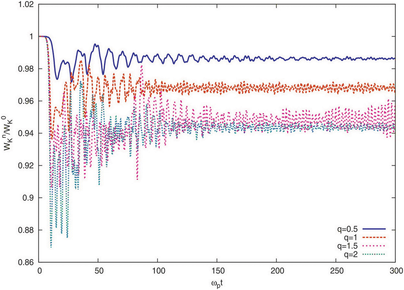
Fig. 5. (Color online) The ratio of kinetic energy of particles to the initial kinetic energy as a function of ωpt for different values of q.
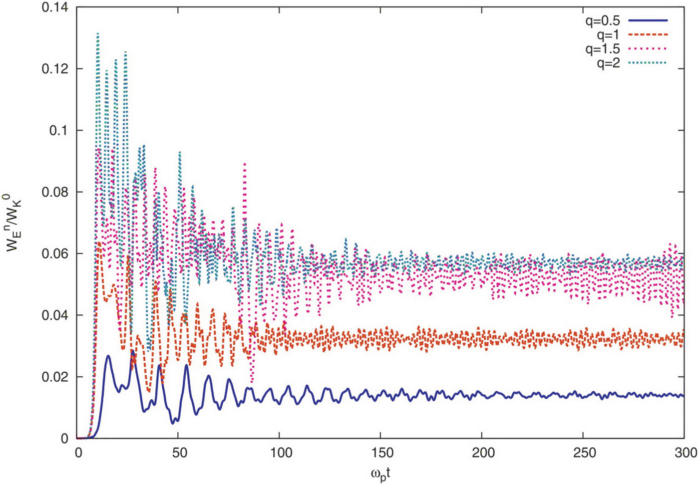
Figure 6 displayed the ratio of electrostatic energy to the initial electrons kinetic energy as a function of ωpt. We see that the electrostatic energy is zero initially, but after a short time around t ≈ 10ωp−1 the system reaches a dynamic equilibrium. After that energy splits between kinetic and electrostatic energies unequally with a continues exchange between two. The energy fluctuations is large when the instabilitystarts, but fluctuations decrease and remain merely constant for sufficiently long time. The maximum energy conversion is related to q = 2 around 15% for time scale around t ≈ 10ωp−1, which in comparison to the Maxwellian distribution the maximum conversion increased by more than twice.

Fig. 6. (Color online) The ratio of electrostatic energy to the particles initial kinetic energy as a function of ωpt for different values of q.
To analyze more the energy conversion process and instability generation, the time development of the electrons velocity-root-mean-square (VRMS) is displayed in Figure 7. We note that the electrons VRMS define as
 $$v_{rms} = \sqrt{\displaystyle{1 \over N_p}\sum\limits_{\,p = 1}^{N_p} \, \lpar \tilde{v}_p^n - \tilde{v}_p^0\rpar ^2}\comma$$
where  $\tilde{v}_p^n$ and
  $\tilde{v}_p^0$ indicate the normalized pth electron velocity at nth time step and t = 0, respectively. The figure shows that the electrons velocity rise rapidly in the time scale that TSI grows (t ≈ 10ωp−1). It is clear that the maximum growth for electrons velocity are belong to the case with entropic indexes q = 2, while the minimum correspond to q = 0.5. The figure approve that the TSI excites strongly when the entropic index q becomes large (q > 1), so electrons are trapped by the field and accelerated quickly up to the large velocities. In addition, it is understood from the Figure 7 that the energy conversion enhances with increasing the entropic index q, which is in agreement of the previous results obtained from simulation. Therefore, the thermal noise can be decrease the electrons VRMS and as the result the energy conversion efficiency and the TSI growth rate.
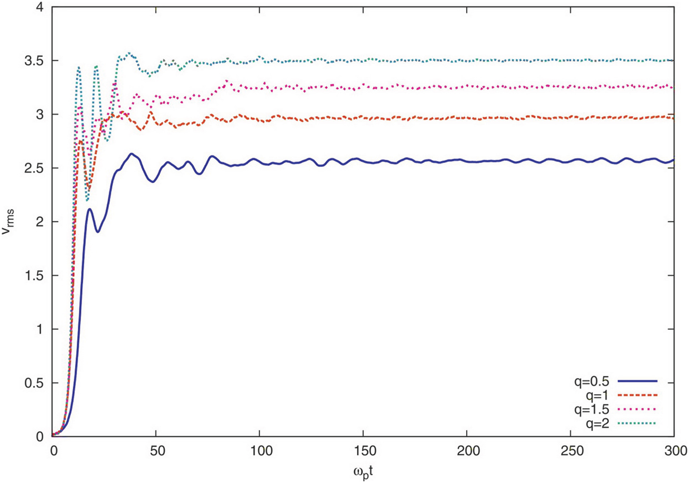
Fig. 7. (Color online) Particles velocity-root-mean-square variation as a function of ωpt for different values of q.
In Figure 8, we display the ratio of electrons total energy to the initial total energy in terms of ωpt for q = 1.5. The energy history clearly approves the energy conserving in our PIC simulation.
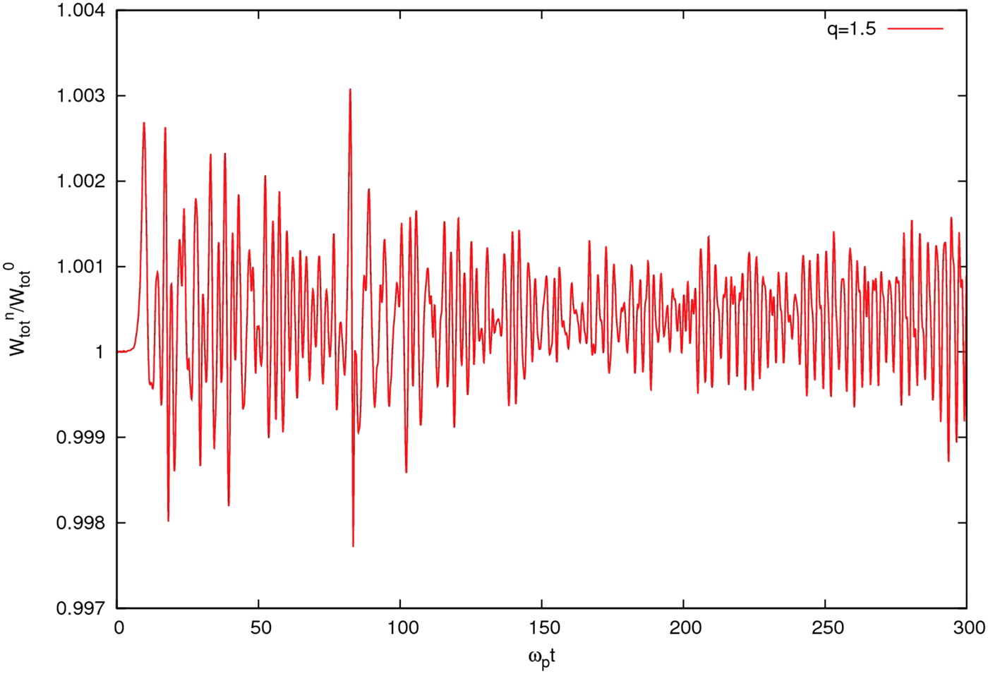
Fig. 8. (Color online) Normalized total energy history for q = 1:5.
4. SUMMARY AND CONCLUSION
In the present, we have performed extensive one-dimensional PIC simulations to investigate TSI driven by two counter streaming symmetric electron beams. We have interpreted our results by a non-extensive q-distributions of Tsallis statistics. The simulation consist one million superparticle equally loaded in two beams propagating in opposite direction. The results indicate that the generation of TSI and cavity formation are dominated by the entropic index q. While for the large values of q > 1 the cavitation was complete, for small q ≪ 1 the cavity formation was not perceptible. The snapshots of excited electric fields in real space clearly show that the strength of the fields are enhanced by increasing the entropic index q. The ratio of electrostatic energy to the electrons initial kinetic energy reveals that the energy conversion and the instability generation are sufficiently predominated by increasing the entropic index up to the values q > 1. Our results suggest that the cavity formation and instability generation can be affected by particle thermal spreading. For example, for a system with entropic index q < 1 the particle velocities speared widely around the drift velocity v 0 = ±3 and the excited fields strength were very weak compared to the cases q > 1, which the velocities spreading were very thin. The normalized total energy history for a arbitrary entropic index q = 1.5, approves the energy conserving in our PIC simulation