


1. INTRODUCTION
Conditions for the development of the Rayleigh-Taylor (RT) instability arise in the Laboratory of Planetary Sciences (LAPLAS) experiment (Tahir et al., 2005) that will be performed at Gesellschaft für Schwerionenforschung (GSI), Darmstadt, Germany, in the frame of the Facility for Antiproton and Ion Research (FAIR) facility (Henning, 2004; Hoffmann et al., 2005). A typical experiment (Fig. 1) considers a cylindrical target in which the sample material (for example, hydrogen) is surrounded by a thick shell of heavy material (typically gold or lead). One face of the target is irradiated with an intense ion beam that has an annular focal spot. When the annular region is heated by the ion beam, it expands, pushing the inner layers of the target (the pusher), and compressing the material sample in the axial region. The external layer around the beam-heated zone acts as a tamper that confines the implosion for a longer time.

LAPLAS (Laboratory of Planetary Sciences) experimental scheme.
By means of numerical simulations and analytical models (Tahir et al., 2001, 2003, 2004; Piriz et al., 2002a, 2002b; Temporal et al., 2005, 2003; Breil et al., 2005), we have shown that this configuration is very suitable for an experiment dedicated to the study of the hydrogen metallization problem (Wigner & Huntigton, 1935; Weir et al., 1996). Such studies include the problem of the generation of the annular focal spot (Arnold et al., 1982; Piriz et al., 2003a, 2003b).
The stability of the pusher during the implosion still remains an issue of possible concern. The RT instability will arise at the pusher/absorber interface during the acceleration phase, and later at the pusher/hydrogen interface during the stagnation phase. Under the conditions of the LAPLAS experiment, the pusher will be accelerated by a driving pressure of few megabars achieving accelerations of the order of 1013 cm/s2. During the implosion, the pusher remains mainly solid although its internal layers are melted during the deceleration phase, so that it retains the elastic and plastic properties during most of the implosion process. On the other hand, the absorber region is melted during the phase of heating and then it remains in a liquid state the rest of the implosion time. Similar situations can be found in magnetically accelerated shells (Bowers et al., 1998; Keinigs et al., 1999; Reinovsky et al., 2002) and in plates accelerated by gaseous detonations products (Barnes et al., 1974, 1980; Bakharakh et al., 1997). Recently, a method based on measuring the RT instability in solids has been proposed to study the material strength of metals at extreme pressures (Colvin et al., 2003; Lorenz et al., 2005).
Some analytical works have been presented to deal with the RT instability in solids (Miles, 1966; White, 1973; Dienes, 1978; Drucker, 1980; Robinson & Swegle, 1989; Nizovtsev & Raevskii, 1991; Bakharakh et al., 1997; Plohr & Sharp, 1998, Colvin et al., 2003; Terrones, 2005; Piriz et al., 2005). Among these works we will focus on a few of them. The first one is the work by Plohr and Sharp (1998). They consider the instability that is developed on a solid/vacuum interface, so that it is limited to the case in which the Atwood number AT = (ρ2 − ρ1)/(ρ2 + ρ1) is equal to 1. The behavior of the solid is modeled as a perfectly elastic solid and, by means of the Laplace transform method, an exact solution is obtained in which the growth rate is given by an implicit formula. Although this model is exact and describes the initial transient phase and the asymptotic regime it is so involved from a mathematical point of view that it seems very difficult to extend it to more realistic situations, for example, the inclusion of plastic behavior. The second one is the work by Terrones (2005). He has obtained an exact solution for arbitrary Atwood numbers that applies to solid/solid and solid/viscous fluid interfaces. In both cases, the solid is considered perfectly elastic. This model is based on a normal mode linear analysis, so that it yields a growth rate that coincides with the results by Plohr and Sharp (1998) (for AT = 1) once the asymptotic regime has been reached. However, this model cannot describe the initial transient phase determined by the initial conditions. The third work is by Piriz et al. (2005). This approximated model can describe the complete time evolution of the perturbation. It is based on the second law of Newton and produces explicit analytical results that are in excellent agreement with the two previous models that are exact but more restrictive in their applications. Moreover, as we will show in this paper, the initial conditions are very important in the further development of the instability. The RT instability can be preceded in practice by the Ritchmyer-Meshkov (Wouchuk, 2001) unstable phase and/or by a ramp in the driving pressure. So a relatively simple model, although approximate, is of great importance in order to include more realistic phenomena like elastoplastic behavior of the solid or finite thickness effects. It is important to highlight that the model by Plohr and Sharp (1998) is valid for any thickness of the solid layer while the one by Terrones (2005) applies only to infinite semi-spaces.
Some efforts have been made in the past for simulating the RT instability in accelerated solids. Two of the most relevant are those by Swegle and Robinson (1989) and Bakharakh et al. (1997). In the first one, an elastoplastic solid slab that is accelerated by means of an external driving pressure is studied. So, the study is restricted to the case of AT = 1. The work consists in an exhaustive parametric study in which the influence of many factors like the wavelength, the initial amplitude, the material properties, the rise time of the driving pressure, etc. are analyzed. One shortcoming of this work is that these researchers dealt with many parameters at the same time and they did not have an adequate analytical model to check and interpret their results. The work by Bakharakh et al. (1997) is the compilation of the Russian papers until 1997 on RT in solids. They performed numerical simulations on semi-spaces with Atwood numbers very close to one, and they also presented some numerical simulations to support the model of Nizovtsev and Raevskii (1991) for a thin elastoplastic shell. The Nizovtsev and Raevskii (1991) model predicts, within the elastic limit, a value of the critical wavelength λc that is in good agreement with the exact model by Plohr and Sharp (1998), and if the plastic flow is taken into account, the stability boundaries seem to agree with some experiments (Dimonte et al., 1998).
In our work, we present a systematic set of numerical simulations on the RT instability in semi-spaces covering the following general cases: elastic solid/elastic solid and elastic solid/viscous fluid interfaces. To simulate semi-infinite media, we consider thick layers of thickness h, so that kh >> 1, where k = 2π/λ is the wave number, and λ is the wavelength of the perturbation of the interface. We compare the results, in terms of the growth rates, with the exact results by Terrones (2005) and with the approximate results (within a 15% of error) by Piriz et al. (2005). In addition, we can incorporate the initial conditions imposed by the simulations in the model by Piriz et al. (2005) and check the excellent performance of this model. Finally we present a few examples showing the importance of taking into account such initial conditions specially if more realistic material models (for example, elastoplastic models) are considered.
2. NUMERICAL MODEL
The numerical calculations have been performed with version 6.5 of the ABAQUS finite element code (Hibbit, Karlsson and Sorensen Inc. Pawtucket, RI) which is suitable for modeling fast transient phenomena. It is based on a central difference scheme for the time integration of the equations of motion of the body. The algorithm has second-order accuracy and is conditionally stable. This means that the time step size is fixed according to stability requirements resulting from the Courant criteria.
The behavior of the material is composed of a volumetric and a deviatoric part. The hydrostatic behavior is governed by an equation of state while the deviatoric behavior is governed by a constitutive law, assuming that these two responses are uncoupled. The material hydrostatic behavior is defined by the Mie-Grüneisen equation of state:

where P and E are the pressure and specific internal energy and Ph and Eh are the Hugoniot pressure, and Hugoniot specific internal energy, respectively. The latter are functions of the material density ρ only. Also Γ is the Grüneisen ratio defined as:

where Γ0 is a constant characteristic of the material and ρ0 is the reference density. On the other hand, the momentum and energy conservation equations are:

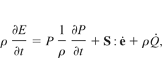
where v is the velocity,

is the rate of change of the deviatoric strain tensor, S is the deviatoric stress tensor, and

is the heat rate per unit of mass.
The equation of state and the equation of energy conservation are coupled through the pressure and the internal energy. The Hugoniot equations relate the pressure, internal energy, and density behind the shock waves to the corresponding quantities in front of them in terms of the shock velocity us, and the particle velocity up. The Hugoniots of many materials can be adequately represented by the following linear relationship (McQueen et al., 1970):

where c0 and s are fitting parameters that depend on the considered material and are experimentally measured.
Three different constitutive laws are considered in this work for the deviatoric part of the model. For a viscous fluid, the deviatoric stresses Sij are related to the deviatoric strain rates

through the viscosity μ

To model a solid that behaves elastically the constitutive law is given by the following linear relationship between the deviatoric stress rates

and the deviatoric elastic strain rates


where G is the shear modulus and dots indicate the time derivatives.
Finally, the deviatoric part of the material can be modeled by using a perfectly elastoplastic model (i.e., the yielding plastic surface does not change with the plastic deformation) with a von Mises yield surface and an associative plastic flow. This model needs two parameters, namely the shear modulus G and the yield strength Y that defines the onset of the plastic range. The algorithm to calculate the stresses checks if the material has reached the plastic regime or if it is within the elastic one. In this last case, the elastic relationship is used and if plasticization occurs, the classical radial return algorithm (Hughes, 1984) for the updating of stresses is applied. Of course, much more realistic models like the Steinberg-Guinan constitutive model (Steinberg et al., 1980), that accounts for the hardening due to increasing pressure, and the softening due to increasing temperature can be used, but for the purpose of this paper, the simple elastoplastic model is sufficient.
The medium to be modeled is shown in Figure 2. It is spatially discretized with four-node plane strain elements. It consists of two thick layers separated by a surface which has a sinusoidal perturbation characterized by the wavelength λ and the initial amplitude ξ0. Both, the upper and lower surfaces are flat and the position of the internal nodes is linearly interpolated between these surfaces and the perturbed interface. The thickness of the layers is h, so that kh >> 1 in order to simulate the instability of semi-infinite media. Moreover, the lateral surfaces have symmetry conditions to model an infinite lateral layer. In order to accelerate the medium an external driving pressure Pext is applied to the top surface; so the acceleration that the medium experiments is

where ρ1 and ρ2 are the densities of the layers, respectively. The driving pressure is applied from 0 to the maximum value Pext in a certain time and then is kept constant. In Figure 2, the time history of the load as well as a typical mesh used in the study are also represented. The particularization to solid/vacuum interface is immediate simply eliminating the upper layer.

Configuration used in the study, showing the layer thickness h, the initial perturbation amplitude ξ, the perturbation wavelength λ and the applied driving pressure P. Also, the finite element mesh is shown.
3. NUMERICAL STUDY
Once the medium is accelerated, the perturbation of the interface can follow one of the following patterns: an unbounded growth that asymptotically becomes exponential (unstable case) or an oscillatory motion after a transient phase (stable case) as shown in Figures 3 and 4. Obviously, in an unstable situation the asymptotic growth rate γ+ is the slope of the time evolution of the perturbation ξ(t) in a semi-logarithmic scale. On the other hand, the frequency of the oscillatory stable pattern is given by γ− = 2π/T with T the period of such an oscillation.

Time evolution of the perturbation amplitude ξ(t) of typical numerical simulations. For an unstable situation the perturbation amplitude experiments an unbounded growth that asymptotically becomes exponential.

Time evolution of the perturbation amplitude ξ(t) of typical numerical simulations. For a stable situation the perturbation amplitude experiments an oscillatory motion after a transient phase.
To perform the numerical simulations, the following data have been used. The wavelength of the perturbation is λ = 2.5 mm, the thickness of both layers is h = λ = 2.5 mm, and the initial amplitude is ξ0 = 5 μm. The quantity kh = 2π is sufficient to simulate an infinite semi-space while such a small value of the initial amplitude assures a linear behavior during a sufficiently long time of computation. The spatial discrimination consists in a grid of 40 × 40 finite elements for each of the two layers.
In all the simulations, the heaviest media is simulated by an elastic material defined by the shear modulus G2. To describe the hydrostatic part we have taken the properties of Aluminum: ρ2 = 2700 kg/m3, c0 = 5380 m/s, Γ0 = 2.16, and s = 1.337 (Swegle & Robinson, 1989). For the lightest medium we need to define the shear modulus G1 (elastic solid) or the viscosity μ1 (viscous fluid). To cover different Atwood numbers some values of the density of the lightest medium ρ1 have been used. The parameters c0, Γ0, and s are the same for both materials. In all the simulations, the acceleration of the gravity g is defined by means of an external pressure Pext with a rise time of trise = 5μs.
The comparisons between the numerical simulations and the analytical results are shown in the following sections. It is important to remark that the comparisons have been made in terms of dimensionless numbers; therefore there are several combinations of material parameters that produce the same results. We have used different values of the shear module G1 and G2 as well as the acceleration of gravity g to define the dimensionless wave number k(G1 + G2)/ρ2 g, and we have verified that the obtained dimensionless growth rate γ+ [(G1 + G2)/ρ2 g2]1/2 does not depend on the particular value of the parameters.
3.1. Asymptotic growth rate
We have calculated the asymptotic instability growth rate by considering two thick media separated by an interface for the case in which both media are perfectly elastic solids and for the case in which one of them is an elastic solid and the other one is a viscous fluid. The results for elastic solid/elastic solid interfaces are shown in Figure 5. We have represented the asymptotic dimensionless growth rate γ+ [(G1 + G2)/ρ2 g2]1/2 as a function of the dimensionless wave number k(G1 + G2)/ρ2 g for two different Atwood numbers, namely AT = 1 and AT = 0.6.

Asymptotic dimensionless growth rate γ+ [(G1 + G2)/ρ2 g2]1/2 as a function of the dimensionless wave number k(G1 + G2)/ρ2 g for two different Atwood numbers, namely AT = 1 and AT = 0.6. Elastic solid/elastic solid interfaces. Solid lines are the model by Terrones (2005), dashed lines are the model by Piriz et al. (2005) and circles are the numerical simulations.
The results for elastic solid/viscous fluid interfaces are shown in Figure 6. We have represented the asymptotic dimensionless growth rate γ+(G2 /ρ2 g2)1/2 as a function of the dimensionless wave number kG2 /ρ2 g for AT = 0.8 and two different values of the dimensionless viscosity parameter m = [μ1 g(ρ2 /G23)1/2]1/2, namely m = 0.1 and m = 2. The results of the numerical simulations (circles) are compared with the exact analytical results by Terrones (2005) and to the approximate analytical results by Piriz et al. (2005) (dashed lines). For both interfaces, it is possible to see that the results of the simulations fit perfectly with the exact results by Terrones (2005) while the approximate results by Piriz et al. (2005) are within a 15% of error.

Asymptotic dimensionless growth rate γ+(G2 /ρ2 g2)1/2 as a function of the dimensionless wave number kG2 /ρ2 g for AT = 0.6 and two different values of the dimensionless viscosity parameter m = [μ1 g(ρ2 /G23)1/2]1/2, namely m = 0.1 and m = 2. Elastic solid/viscous fluid interfaces. Dots are the model by Terrones (2005), dashed lines are the model by Piriz et al. (2005) and circles are the numerical simulations.
3.2. Effective initial amplitude (initial conditions)
The asymptotic regime in which the perturbation grows exponentially with a growth rate γ+ is achieved after a transient phase that lasts for a time of the order γ+−1. Although this growth rate is independent of the initial conditions, the perturbation amplitude will be affected, in general, by the initial velocity

and the initial acceleration

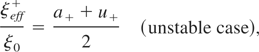
. These initial conditions are important because the RT phase may start from a surface at rest in a stress-free material or, instead it may arise after a transient phase in which the driving pressure increases before reaching a constant value. Therefore, the description of the transient phase between the initial conditions and the asymptotic regime is essential in order to determine the perturbation amplitude at any time. In particular, the effective initial amplitude ξeff from which the perturbation seems to growth when the asymptotic regime is reached may be very different from the real initial perturbation ξ0. The meaning of the effective initial amplitude is clearly shown in Figures 7 and 8. For an unstable case, the effective initial amplitude ξeff+ is the apparent amplitude for which the time evolution of the perturbation would start if it were asymptotic from the beginning. For a stable case, the effective initial amplitude ξeff− is the amplitude of the oscillation.

Graphical representation of the dimensionless effective initial amplitude. For an unstable case, the effective initial amplitude ξeff+ is the apparent amplitude for which the time evolution of the perturbation would start if it were asymptotic from the beginning. This case has been computed according to the model by Piriz et al. (2005) for the particular values of u+ = 5 and a+ = 5.

Graphical representation of the effective initial amplitude. For a stable case, the effective initial amplitude ξeff− is the amplitude of the oscillation. This case has been computed according to the model by Piriz et al. (2005) for the particular values u− = 5 and a− = 5.
In Piriz et al. (2005) the dimensionless effective initial amplitude ξeff±/ξ0 was compared to the exact results by Plohr and Sharp (1998) with an excellent agreement. It is important to highlight here that the results by Plohr and Sharp (1998) apply to a stress free plate initially at rest, so that

. This is not the case of our simulations in which the rise time of the driving force imposes different initial conditions (initial conditions are taken at the end of the ramp of the load). We have measured in the computations the velocity

and the acceleration

at the end of the rise time of the pressure, and then we used them to obtain the dimensionless effective initial amplitude ξeff±/ξ0 that is given according to the model by Piriz et al. (2005) by the following expressions:

where

. In Figures 7 and 8, the time evolution of the perturbation is calculated according to the model by Piriz et al. (2005) for the particular cases of u± = 5 and a± = 5.
In Figures 9 and 10, the dimensionless effective initial amplitude ξeff±/ξ0 versus the dimensionless wave number 2kG2 /ρ2 g is represented for the unstable and stable cases respectively. In these cases, we have considered a solid/vacuum interface that is AT = 1. We can see that the numerical simulations (circles) fit quite well with the approximate analytical results by Piriz et al. (2005) (crosses).

Dimensionless effective initial amplitude ξeff+/ξ0 versus the dimensionless wave number 2kG2 /ρ2 g for an unstable case. Solid/vacuum interface. Circles are the numerical simulations and crosses are the analytical results by Piriz et al. (2005).

Dimensionless effective initial amplitude ξeff−/ξ0 versus the dimensionless wave number 2kG2 /ρ2 g for a stable case. Solid/vacuum interface. Circles are the numerical simulations and crosses are the analytical results by Piriz et al. (2005).
It is important to note that this effective amplitude goes to infinity when the perturbation wave number approaches the cutoff value (k → kc = ρ2 g/2G2), where the growth rate γ goes to zero. In this kind of situations, the instability could enter in the nonlinear phase or in the plastic flow before the asymptotic regime is reached.
3.3. Importance of the initial transient phase with an elastoplastic behaviour for the solid layer
In this section, we show the importance of the initial phase when we consider a more realistic constitutive law to model the solid behavior, for example, a perfectly elastoplastic law.
We have simulated a solid/vacuum interface (AT = 1) with material and geometric parameters that lead to a stable, oscillatory pattern if the solid is considered to behave elastically. Two different rise time of the driving pressure have been taken into account. As Figure 11 shows, the amplitude of the oscillation is larger for the shorter rise time. We fix the elastic limit in such a way that only this evolution enters in the plastic regime. The case of the longer rise time will continue behaving elastically (so it will remain stable) but the case of the shorter rise time will plastify and will develop an unstable growth.

Time evolution of the perturbation ξ(t) for two different rise time of the driving pressure. For elastic materials both evolutions follow a stable pattern but if an elastoplastic material law is taken into account, the case of the longer rise time is stable while the case of the shorter rise time is unstable.
The same situation can be observed in Figure 12. Now the difference is the initial amplitude of the perturbation. The case in which the initial amplitude is larger will oscillate with larger values and therefore it can reach the plastic regime (and it becomes unstable) while the other case will remain elastic and stable.

Time evolution of the perturbation ξ(t) for two different initial perturbation amplitudes. For elastic materials both evolutions follow a stable pattern but if an elastoplastic material law is taken into account, the case of the smaller initial amplitude is stable while the case of the larger initial amplitude is unstable
In both cases the RT instability has entered in the plastic regime before the elastic asymptotic regime has been reached.
4. SUMMARY AND CONCLUSIONS
In this paper, numerical simulations of the RT instability in infinite semi-spaces (kh >> 1) considering elastic solid/elastic solid and elastic solid/viscous fluid interfaces have been done. The results of the simulations fit quite well with previously published analytical models. In particular, the asymptotic growth rate has been compared with the exact model by Terrones (2005) and with the approximated model by Piriz et al. (2005). The initial transient phase before reaching the asymptotic regime has been compared, with excellent agreement, with the model by Piriz et al. (2005). The initial phase is of great importance because the instability can enter in the non-linear phase or in the plastic flow before the asymptotic regime is reached. We have presented some few examples showing this effect. Therefore, to fix the stability boundaries with an elastoplastic model, the actual values of the perturbation at any time (not only in the asymptotic regime) are needed.
ACKNOWLEDGMENTS
This work has been partially supported by the Ministerio de Ciencia y Tecnologìa (DPI2005-02278; FTN2003-00721), by the Consejerìa de CYT-JCCLM (PAI-05-071) of Spain and by the BMBF of Germany.


