1. INTRODUCTION
Since Read (1984) and Youngs (1984) published the first experimental study of
Rayleigh–Taylor instability with a randomly perturbed fluid
interface, attention has been drawn to the nondimensional acceleration
rate of the bubble envelope. Assume that two fluids are separated by a
randomly perturbed interface and that the gravitational field points
from the heavy fluid ρH to the light fluid
ρL. Read and Youngs confirmed the
Sharp–Wheeler theoretical prediction (1961,
unpublished technical report, Institute of Defense Analyses) that the
average bubble front moves with acceleration scaling
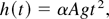
where h is the height of the bubble envelope, A =
(ρH −
ρL)/(ρH +
ρL) is the Atwood number, g is the
gravity, and t is time. Read (1984)
and Youngs (1984) show that the acceleration
rate α is almost a constant, with α ≈ 0.063 − 0.077 in
three-dimensional (3D) experiments. The experiments have been repeated
by various authors with different apparatus, and similar values of
α have been obtained; we mention the experiments of Dimonte and
Schneider (1996, 2000
and Dimonte (1999)), giving α = 0.05 ±
0.01. The theoretically determined value, α ≈ 0.05–0.06, is
obtained from a bubble merger renormalization group model. See B. Cheng, J.
Glimm, and D.H. Sharp (in press), and references
cited there. Computation of the center of mass of the mixing zone introduces
a coupling between its two edges. Therefore, a characterization of the center
of mass (nearly stationary for A ≤ 0.8, e.g.) determines the total
mixing zone size in terms of α alone (Cheng, et al., 1999, 2000).
The coefficient α is thus important. It characterizes the size of
the mixing zone, and thus largely determines the amount of material
that is mixed. It has been reported by experimentalists as being
approximately universal, in the sense that it is nearly independent of
the random initial conditions of an experiment.
Researchers in several laboratories have tried to reproduce the
Sharp–Wheeler theoretical scaling law with the experimental value
for α through numerical simulation. Most researchers report a
time-dependent, decreasing value for α, ranging from 0.015 to
0.03.
These simulations are from computational codes using numerical
schemes with interfacial mass diffusion. We have compared numerical
simulations using a high resolution front tracking code
FronTier with zero interfacial mass diffusion to our own
simulations using an untracked total variation diminishing (TVD)-level
set code with interfacial mass diffusion similar to the others. We also
introduce an analytic study of the effects of mass diffusion on
buoyancy reduction and we predict the numerically observed reduction in
α for untracked simulations. Our main result is that all values of
α (theory, experiment, simulation) are consistent if the diffusive
calculation of α is renormalized to account for mass diffusion.
We also performed simulations of the Richtmyer–Meshkov
instability in spherical geometry using a two-dimensional (2D)
cylindrical code.
2. DIFFUSIVE AND NONDIFFUSIVE SIMULATIONS
An earlier comparison shows that FronTier simulations
produce values for α close to agreement with experiment while
untracked TVD simulations produce low values for α (see Glimm et al., 2001). These comparisons
were limited in the simulation time and in the penetration depth of
mixing achieved. Here we extend the comparison to a later time,
comparable to most other simulations. Figure
1 shows the evolution of the fluid interface in the
FronTier simulation. The color coding displays the height
through the mixing zone, and the cut plane near the bubble surface at
the top of the right frame shows the location of the 5% volume fraction
contour for the light fluid. Note that there are a number of light
fluid bubbles at the later time. The dynamics is multimode, not
dominated by a single large space filling bubble up to this time. Such
a large bubble would indicate the end of any possible self-similar flow
regime, as the acceleration scaling depends upon a continued growth in
the transverse scale of the mixing structures. We expand on this idea.
The dynamics of continued acceleration of the mixing zone edge, as
expressed in the t2 scaling in Eq. (1), depends on
a continued growth of the large scale structures (the bubbles). See,
for example, Sharp (1984). Bubbles grow
through a process of bubble competition and merger. Thus the
t2 scaling and the determination of α requires
a simulation that is still in the multimode regime, where bubble
competition and merger can occur.
Front plot for a FronTier simulation of
Rayleigh–Taylor mixing, with A = 0.5. Left frame: early
time. Right frame: late time. Color coding represents vertical height.
The initial mean height of the interface is 4, and the height scale on
the color bar applies only to the later time.
The t = 0 interface is constructed out of Fourier modes with
random amplitudes and frequencies in the range of 8 to 16 modes per
computational domain width. See Glimm et al. (2000) for further information concerning these
simulations. The 2 × 2 × 8 computational domain used here
allows computationally efficient late time, deep penetration
simulations.
Within this computational aspect ratio, the Fourier mode numbers
represent a balance between the conflicting requirements of spatial
resolution, favoring low numbers of modes, and late time statistical
validity, favoring large numbers of modes. Except as noted, the
simulations used a 1282 × 512 grid. Our simulations,
thus balanced, have about 122 = 144 initial bubbles and a
grid resolution of about 10 cells in each dimension per initial bubble.
The final time considered here has about five bubbles (see Fig. 1).
A comparison of the mixing rates for the two simulations is shown in
Figure 2 (left), plotting bubble height
h versus Agt2. FronTier has a
distinctly higher growth rate than does the interface mass diffusive
TVD simulation. The value of h(t) is the difference
between the t = 0 bubble height and the time t bubble
height. The latter quantity is defined in terms of a 1% volume
fraction, that is, the greatest height at which the fluid is 99% heavy
and 1% light according to the front tracking front or the TVD level
set. This definition is somewhat unstable statistically, and a few
spurious oscillations associated with the definition were removed in
the plots of Figure 2.
Mixing growth comparison of a FronTier (nondiffusive) with a
TVD (diffusive) simulation. For the TVD simulation, two grid levels are
shown, the coarser being 642 × 128. In all cases,
h is the height of the 1% volume fraction contour, and the
initial mean height of the interface is 4. Left: h versus
A(t = 0)gt2 for FronTier
and TVD. Right: h versus
for FronTier and TVD. The solid line represents the
FronTier simulation, the dashed line is the finer grid TVD
simulation, and the dotted line is the coarser grid TVD simulation.
Mass diffusion is a common feature of most untracked simulation
codes. Due to the interpolation constraint, numerical schemes (finite
difference, finite volume) can have only first order accuracy in their
spatial derivatives near a discontinuity. For a contact discontinuity,
the corresponding characteristic is linear for the wave equation of the
Riemann invariant
and so the truncation error will spread to the interior region.
Assuming that a finite difference scheme is second order in time and
first order in space at a contact discontinuity, we have the equivalent
equation
so that the width ΔL of the numerically diffused density
profile satisfies
.
To understand the difference between the two simulations, we compare the
cross-sectional density plots in a series of horizontal slices from the
bubble (upper) portion of the mixing region. Figure
3 shows the cross-sectional density plots in these simulations.
Observe that there is a substantial smearing out of the density across
the boundary between the two fluids in the untracked TVD simulation,
whereas the FronTier simulation maintains a sharp boundary
with a discontinuous density profile throughout the simulation. As a
further difference, we note the fine-scale structure size in the
FronTier simulation in comparison to the TVD simulation.
Cross-sectional plots showing density on a common rainbow color
scale. The pure light fluid is colored blue and the pure heavy fluid is
red. Yellow and green represent various levels of microscopic mixing.
The ratio of extreme density values is 3.3:1. The right frames show a
higher slice in the z direction. Top: FronTier,
bottom: TVD. The simulations are shown at comparable penetration
distances, but at different times (Agt2 = 23 for
FronTier, Agt2 = 66 for TVD). It is
evident that the density contrast for the TVD simulation has been
reduced by about 50% due to mass diffusion. See also Figure 4.
We compute an effective Atwood number A(t) as a
function of time for the TVD simulations. This is determined from the
highest and lowest densities in a horizontal slice, with the resulting
time- and space-dependent Atwood number averaged over heights in the
upper third of the mixing zone at a fixed time to get an Atwood number
dependent on time alone.
Time-dependent A (Atwood number) for fine grid
FronTier, fine grid TVD, and coarse grid 642
× 128 TVD. At time t = 0, all three simulations have
A(t = 0) = 0.5. This plot displays the reduced
buoyancy of the diffusive TVD simulations as a function of time.
In Figure 4, we plot A(t)
versus t for three simulations (fine and coarse grid TVD and
fine grid FronTier). The time dependence of
A(t) in the FronTier simulation is caused
purely by (small) compressibility effects. For the mass diffusive TVD
simulation, the initial density contrast, A(t = 0) =
0.5, is almost completely washed out; the earliest time displayed shows
A(t = 2) ≈ 0.15. As new pure (heavy and light)
fluid is injected into the mixing region, the effective Atwood number
increases, but it is still reduced to about A ≈ 0.3 on a
time averaged basis, or nearly a 50% reduction relative to its initial
value.
To compensate for the time-dependent Atwood number
A(t), we define an effective alpha,
αeff ≈ h/2 ∫∫
A(s)g ds dt (see Fig. 2, right). Specifically, α or
αeff is defined here as the slope of the
straight line joining the beginning and end of the
h(t) curve in Figure 2.
This definition, although somewhat arbitrary, is conventional, and thus
allows comparison to the results of others. We observe an improved
comparison between FronTier and TVD and between TVD and
experiment. Note that αeff lies within the
range of experimental values; see Table 1. On
this basis, we can state that the diffusive buoyancy renormalization of
α is capable of resolving existing discrepancies among simulations,
between diffusive simulations and nondiffusive experiments, and with
theory.
Values of α determined from experiment, theory, and
simulation
3. DIFFUSION INDUCED BUOYANCY REDUCTION
The reduced mixing rate due to unphysical numerical diffusion can be
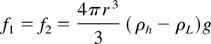
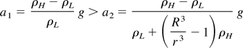
understood from Figure 5. The left frame
represents an immiscible bubble of radius r. The central and
the right frame assume that this bubble is smeared out numerically to a
radius R whereas the total mass inside the sphere of radius
R is conserved. The buoyancy forces
Left: Unmixed bubble of light fluid. Center: Unmixed bubble and heavy
fluid mass that will be mixed with it. Right: Mixed bubble.
for the bubbles in frames (a) and (c) are the same. However, due to
the difference between the mass in the nondiffused bubble (a) and the
diffused bubble (c), the two acceleration rates
are different.
As a result of the mass diffusion, the buoyancy force is distributed
to a larger amount of mass, thus reducing the acceleration of the
bubble.
4. RICHTMYER–MESHKOV INSTABILITY
We have performed verification and validation studies for
axisymmetric simulations using Fon Tier. The validation was
through comparison to laser driven hemispherical targets (Cheng et al., 2000), and will not be
repeated here. In Figure 6, we present the results of a mesh refinement
study for an axisymmetrically perturbed spherical Richtmyer-Meshkov
problem, comparing the growth rates as a function of time for a 200 ×
200 and a 400 × 400 mesh. The influence of the symmetry axis (the
“North Pole” effect on the statistical characterization of the
instability evolution was studied (Glimm et al.,
2000; in press a; in press b), with the main conclusions that: (1)
the effect was a real consequence of axisymmetrically perturbed flows, i.e.,
it was not due to numerical effects, (2) it was independent of spherical flow
geometry, and arises in cylindrically shaped flows, (3) that the effect occurs
late in time and for spherical flows, is pronounced after reshock, and (4)
that the effect is not eliminated through use of spherical harmonic (Legendre
polynomial) perturbations.
We present in Figure 7 the results of a strong shock scaling law analysis
of the mixing zone growth rate for a spherically perturbed Richtmyer-Meshkov
problem. The perturbed spherical surface separates a heavy gas (on the
interior) from a light gas (on the exterior), with the initial shock location
in the heavy fluid, facing outward (explosion). Following Zhang and Graham
(1997), where a similar scaling law was introduced
for cylindrical implosions, we scale the velocity and times by the
incident shock Mach number, introducing a scaled velocity
v′ = v/M and time
t′ = Mt. The results of the scaling show a near
identity of growth rate curves, which is remarkable in view of the
large amount of structure in the curves themselves. Again the
configuration is heavy exploding light.
5. CONCLUSION
We present a FronTier simulation run to late time and deep
penetration. The simulation is terminated while still in a multimode
regime. It has no interfacial mass diffusion, and the overall bubble
mixing rate lies within the experimental range. We recalibrate the
buoyancy force for mass diffusive TVD simulations, and obtain a
renormalized αeff that is also in agreement
with experiment. On this basis, the nondiffusive simulation and the
theory of mass diffused buoyancy reduction presented here are capable
of resolving the principal differences between simulation and
experiment for Rayleigh–Taylor mixing. Our results confirm the
earlier agreement between theory and experiment (see B.
Cheng, J. Glimm, and D. H. Sharp, in press). Finally, we observe
that our results open a door to further research, and do not close inquiry
related to the determination of the mixing rate, as the uncertainties in
the experimental, theoretical, and simulation determination of α
deserve further investigation. Concerning simulation, which is the main
thrust of this article, we mention the importance of improved
resolution. The needs for resolution are numerical accuracy, governed
by mesh cells per bubble, statistical accuracy, governed by the number
of bubbles, especially at the end of the simulation, and convergence to
self-similar flow, governed by the length of time of the simulation.