


INTRODUCTION
Electron heat conduction plays a major role in inertial fusion physics, because it carries the deposited laser energy from the critical surface to the ablation front (Lindl, Reference Lindl1995; Lindl et al., Reference Lindl, Amendt, Berger, Glendinning, Glenzer, Haan, Sunahara, Delletrez, Stoeckl, Short and Skupsky2003; Atzeni & Meyer-ter-Vehn, Reference Atzeni and Meyer-Ter-Vehn2004; Gupta & Godwal, Reference Gupta and Godwal2001). The calculation of the electron transport influences the laser deposition and plasma status inside the hohlraum, it further influences the plasma emission, the laser plasma interaction and the radiation uniformity of the capsule placed in the center of the hohlraum, and finally, it significantly influences the ignition. Therefore, worldwide experimental and theoretical efforts on electron transport in plasmas are in progress (Sunahara et al., 2003; Colombant et al., Reference Colombant, Manheimer and Busquet2005; Shurtz et al., Reference Shurtz, Nicolai and Busquet2000), especially in recent initial ignition campaign at the National Ignition Facility (Lindl & Moses, Reference Lindl and Moses2011; Haan et al., Reference Haan, Lindl, Callahan, Clark, Salmonson, Hammel, Atherton, Cook, Edwards, Glenzer, Hamza, Hatchett, Herrmann, Hinkel, Ho, Huang, Jones, Kline, Kyrala, Landen, MacGowan, Marinak, Meyerhofer, Milovich, Moreno, Moses, Munro, Nikroo, Olson, Peterson, Pollaine, Ralph, Robey, Spears, Springer, Suter, Thomas, Town, Vesey, Weber, Wilkens and Wilson2011; Rosen et al., Reference Rosen, Scott, Hinkel, Williams, Callahan, Town, Divol, Michel, Kruer, Suter, London, Harte and Zimmerman2011). Up to now, various theoretical models have been developed for electron transport, such as the classical electron transport model of Spitzer-Härm (Reference Spitzer and Härm1953; Cohen et al., Reference Cohen, Spizer and Routly1950), the flux limit model (FL model) (Malone et al., Reference Malone, McCrory and Morse1975), the nonlocal electron transport model (Luciani et al., Reference Luciani, Mora and Virmont1983), and the non-Maxwellian model (Huo et al., Reference Huo, Lan, Gu, Yong and Zeng2012). Among all these models, the FL model is the most widely used one in calculating the electron heat flux in hohlraum simulations codes, like LASNEX (Zimmerman & Kruer, Reference Zimmerman and Kruer1975), HYDRA (Marinak et al., Reference Marinak, Tipton, Landen, Murphy, Amendt, Haan, Hatchett, Keane, McEachern and Wallace1996), FCI2 (Buresi et al., Reference Buresi, Coutant, Dautray, Decroisette, Duborgel, Guillaneux, Launspach, Nelson, Patou, Reisse and Watteau1986), and LARED-H (Pei, Reference Pei2007). In the last decades, numerical experiments are designed with FL model (flux limiter) and good results were obtained (Li et al., Reference Li, Lan, Meng, He, Lai and Feng2010; Lan et al., Reference Lan, Gu, Ren, Li, Wu, Huo, Lai and He2010, Reference Lan, Fill and Meyer-ter-Vehn2004; Cook et al., Reference Cook, Kozioziemski, Nikroo, Wilkens, Bhandarkar, Forsman, Haan, Hoppe, Huang, Mapoles, Moody, Sater, Seugling, Stephens, Takagi and Xu2008; Seifter et al., Reference Seifter, Kyrala, Goldman, Hoffman, Kline and Batha2009; Orlov et al., Reference Orlov, Denisov, Rosmej, Schaefer, Nisius, Wilhein, Zhidkov, Kunin, Suslov, Pinegin, Vatulin and Zhao2011). In the FL model, a flux limiter f e is taken to make sure that the flux does not exceed the limit of the free streaming heat flux Q f, and the heat flux is often computed either as min(Q SH, f eQ f) or in a “parallel connection” formulation [Q SH−1 + (f eQ f)−1]−1, where f e is often chosen from 0.05 to 0.15 (Atzeni & Meyer-ter-Vehn, Reference Atzeni and Meyer-Ter-Vehn2004; Rosen & Nuckolls, Reference Rosen and Nuckolls1979; Kline et al., Reference Kline, Glenzer, Olson, Suter, Widmann, Callahan, Dixit, Thomas, Hinkel, Williams, Moore, Celeste, Dewald, Hsing, Warrick, Atherton, Azevedo, Beeler, Berger, Conder, Divol, Haynam, Kalantar, Kauffman, Kyrala, Kilkenny, Liebman, Le Pape, Larson, Meezan, Michel, Moody, Rosen, Schneider, Van Wonterghem, Wallace, Young, Landen and MacGowan2011). In recent theoretical work done for the National Ignition Campaign (Rosen et al., Reference Rosen, Scott, Hinkel, Williams, Callahan, Town, Divol, Michel, Kruer, Suter, London, Harte and Zimmerman2011), a flux limiter of 0.15 was finally taken in the ignition design after comparing with the nonlocal model. However, the choice of f e depends on the hohlraum and the laser parameters used in the study. Hence, it is necessary to find a way to determine f e experimentally for different designs.
In fact, the heat flux may be dominated by the limited free-stream flux in the regions with a steep temperature gradient, including the laser deposition region, the flux-heated overcritical region, and the laser channel boundary between the hot laser plasmas and the surrounding radiation ablated plasmas, while these are important X-ray emission regions. As a result, the choice of f e may influence the laser spot motion and the wall plasma expansion, and therefore influence the motion of the emission regions. Therefore, it is possible to determine f e via the diagnostics of the X-ray emissions. In this paper, we will study the influence of the electron flux limiter f e on hohlraum plasmas by using a two-dimensional (2D) radiation hydrodynamics code LARED-H, and we will propose a method to experimentally determine f e via the motion of the M-band (>1.5 keV) emission region in Au hohlraum.
The hohlraum and laser parameters used in this study are taken from the experiments done by Huser et al. (Reference Huser, Courtois and Monteil2009). In their experiments, the authors measured the wall and laser spot motion in the empty, propane filled, and CH-lined Au hohlraums on the Omega laser facility, and compared the experimental results with their simulations with the 2D radiation hydrodynamics code FCI2. Huser et al. (Reference Huser, Courtois and Monteil2009) observed the wall motion by using axial 2D X-ray imaging and observed the laser spot motion perpendicularly through a thinned wall using streaked hard X-ray imaging. Their experiments gave valuable quantitative results, which are worthy to be compared with the 2D simulations. We will mainly simulate the empty hohlraum used in the experiments (Huser et al., Reference Huser, Courtois and Monteil2009) with different f e and choose a suitable f e by comparing our simulations with the observed motion of the X-ray emission regions. Using the chosen f e, we will also simulate the gas-filled hohlraum used in the experiments of Huser et al. (Reference Huser, Courtois and Monteil2009) and study the effect of gas filling on the wall plasma expansions.
The paper is organized as follows. In Section 2, we will introduce the code and model used in our study. In Section 3, we will use the LARED-H to simulate the empty hohlraum used in Huser's et al. (Reference Huser, Courtois and Monteil2009) experiments with different f e and study the influence of f e on plasma status. In Section 4, we will study the influence of f e on the X-ray emission region in the overcritical plasmas. In Section 5, we will study the influence of f e on the X-ray emission from the plasma corona. In above simulations and discussions, we mainly focus on the empty hohlraum. In Section 6, we study the effect of gas filling on the wall plasma expansion in the gas-filled hohlraum used in Huser's et al. (Reference Huser, Courtois and Monteil2009) experiments. Finally, we will present a summary in Section 7.
2. CODE AND MODEL
The LARED-H is a 2D radiation hydrodynamics code for laser target coupling and hohlraum physics study, which is one of the main simulation codes in designing and analyzing the hohlraum experiments on SGII and SGIII Prototype laser facilities (Li et al., Reference Li, Huo and Lan2011; Huo et al., Reference Huo, Ren, Lan, Li, Wu, Li, Zhai, Qiao, Meng, Lai, Zheng, Gu, Pei, Li, Yi, Song, Jiang, Yang, Jiang and Ding2010). The three-temperature hydrodynamic equations in LARED-H are:
Here, the subscripts e, I, and r indicate electron, ion, and radiation, respectively; the symbol ρ denotes the mass density, u is the flow velocity; T is the temperature; P is the pressure, and q is the artificial viscosity; C ve and C vi are the specific heats of free electron and ion, respectively; W p is the work term due to pressure; W f is the thermal conduction term; W er is the electron-radiation energy exchange term; W ei is the electron-ion energy exchange term; and E r is the radiation energy density; W l is the laser energy deposition via inverse bremsstrahlung and is calculated with a three-dimensional ray-tracing package. An average-atom atomic physics model is included in the code, and the following atomic processes are involved: (1) collisional excitation and de-excitation, (2) spontaneous emission, (3) collisional ionization and three-body recombination, (4) photon ionization and radiative recombination, (5) dielectron capture and auto-ionization.
The expressions of the above energy terms are:

Here, m e is the electron mass; m i is the ion mass; e is the electron charge; ln Λei is the Coulomb logarithm for collisions between electrons and ions; k B is the Boltzmann constant; z is the average ionization degree; N i is the ion density, and N e is the electron density; W bf, W bb, and W ff represent the energy exchanges due to free-bound, bound-bound and free-free transitions of atomic processes, respectively. The electron heat flux Fe taken in our code is the minimum of the S-H flux11F SH and the limited free-stream heat flux f eF l, here F l is the free-stream heat flux.
In LARED-H, the thermodynamic quantities are derived either from the ideal gas model or from data of realistic equation of state. The mean opacity is calculated with relativistic F SH self-consistent average-atom-model OPINCH (Serduke et al., Reference Serduke, Minguez, Davidson and Iglesias2000) where the contributions from free-free, free-bound, and bound-bound transitions are taken into account.
We had used LARED-H to simulate the laser spot moving experiment on NOVA2. In the experiment, a 1 ns flat-top laser pulse was used to drive a hohlraum of 2500 µm in length and 1600 µm in diameter with one laser entrance hole of 800 µm diameter at each end. From LARED-H, the relationship between the laser power P L and the angular velocity dθ/dt of the emission center seen by capsule is ![]() , which is obtained by using the least square method.
, which is obtained by using the least square method.
In this work, the hohlraum and laser parameters used are taken from the experiments done by Huser et al. (Reference Huser, Courtois and Monteil2009). Both empty and propane-filled hohlraums are considered. The cylindrical Au hohlraum is 1.5 mm long with 1.6 mm diameter, with a full-open laser entrance hole at each end. The hohlraum wall thickness is taken as 25 µm. The laser pulse of about 9.5 kJ in total has the shape of Omega PS26N01A with 1 ns pre-pulse followed by 1.5 ns main-pulse with 5:1 contrast. The thirty laser beams simultaneously irradiate the hohlraum from two ends, with respectively, 10 beams at an incidence cone of 42° angle and 20 beams at 59° angle. In our 2D simulations, the widths of both laser rings at 42° and 59° are taken as 400 µm on the inner wall of hohlraum. The laser rings at 42° from two sides not only overlap each other at the hohlraum center, but also overlap the rings at 59° from the same side at about z = 200 µm. Here, z is the axial position from hohlraum center. Thus, the middle part of the hohlraum wall, around 600 µm in length, is fully under the irradiation of the laser. In addition, the initial width of the first Lagrangian cell on the inner surface of wall is taken as 10 nm and the initial temperature of the hohlraum is taken as 300 K. For the empty hohlraum, a pseudo-gas of Au with 8 × 10⁻⁴ g/cm3 initial density is used, and it is assumed that there is no laser deposited in the pseudo-gas. For the X-ray emissions, same as in the experiments (Huser et al., Reference Huser, Courtois and Monteil2009), we also focus on O-band (about 450 eV), N-band (about 800 eV) and M-band (>1.5 keV) and use the same spectral responses for these three bands.
3. HOHLRAUM PLASMA STATUS UNDER DIFFERENT FLUX LIMITERS
The electron conduction carries the deposited laser energy from the critical surface to the over-critical plasma and the plasma corona, so the calculation of the heat conduction influences the plasma status and the X-ray emissions inside hohlraum. In this section, we study the 2D simulation results of the empty hohlraum model and compare the hohlraum plasma status under different f e. From our simulations, the results are sensitive to f e when f e is smaller than 0.1, but insensitive when f e > 0.1. Therefore, we mainly present below the results with f e = 0.05 and 0.1.
First, one should know in which regions the heat conduction is limited by the flux limiters inside hohlraum. In Figure 1, we present the 2D maps of the laser energy deposition term W l and the areas in which the heat flux is dominated by the limited free-stream flux f eF l with respective to f e of 0.05 and 0.1, at 1 ns when the pre-pulse ends while the main pulse starts. The pulse shape of drive laser is also presented in Figure 1a. As shown, the heat flux is dominated by f eF l in the regions with steep temperature gradient, including the laser deposition region, over-critical plasma region and the laser channel boundary between the hot laser plasmas and the surrounding radiation ablated plasmas, which are important regions for the X-ray emissions. However, the limited regions are narrower at a higher f e. When f e is taken as 0.2, from our simulations, the heat conduction is mainly dominated by the S-H flux almost in the whole hohlraum. Notice that f eF l dominates the heat conduction also in the pseudo-gas and at the boundary between the pseudo-gas and the laser channel, but we do not concern these regions that are related to the pseudo-gas in this paper. From our simulation, the plasma-filling is not serious even at the peak laser time. Thus, the laser is mainly deposited near wall for this model.
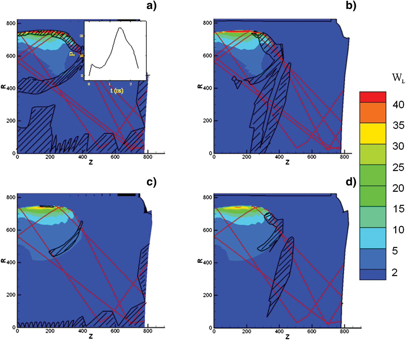
Fig. 1. (Color online) 2D maps of the laser energy deposition term W l (1015 W/m3) and the areas in which the heat flux is dominated by f LF l along, respectively, the ![]() direction (left images) and the
direction (left images) and the ![]() direction (right images), at 1 ns with f e = 0.05 (upper images) and 0.1 (lower images), in which the red lines represent the laser pass. The directions of
direction (right images), at 1 ns with f e = 0.05 (upper images) and 0.1 (lower images), in which the red lines represent the laser pass. The directions of ![]() and
and ![]() are defined for 2D simulation, which are time-dependent and related to cells. The initial directions of
are defined for 2D simulation, which are time-dependent and related to cells. The initial directions of ![]() and
and ![]() are in
are in ![]() and
and ![]() , respectively. The inner plot in (a) is the pulse shape of drive laser.
, respectively. The inner plot in (a) is the pulse shape of drive laser.
Now, we study and compare the plasma status along the laser channel under different f e. Because the laser energy at the 59° angle is two times as large as that at the 42°, so we mainly focus on the laser channel at 59°. In Figures 2 and 3, we present the distributions of T e, n e, and ionization degree Z eff along the laser channel at 59° at 1.7 ns, just after the laser begins to fall and the radiation temperature T r in the hohlraum reaches its peak. As shown, the maximum T e at f e = 0.05 is about 400 eV higher than at f e = 0.1, Z eff at R c is about 1.5 higher, and both R c and the ionization front are around 10 µm closer to wall. Here, R c is defined as the critical position at n e/n c = 1. The reason for a higher maximum T e at a smaller f e is that less energy is conducted to the overcritical region and less mass ablated from wall when the heat conduction is more limited. As a result, at a smaller f e, the laser ablated plasmas are hotter and expand faster along the radial direction, resulting in a lower n e in the plasma corona. Obviously, the critical position and the ionization front move slower towards the hohlraum axis at a smaller f e.

Fig. 2. (Color online) The distributions of T e along the laser pass of the 59° beams at 1.7 ns with f e of 0.05 (black), 0.1 (red) and 0.2 (blue).

Fig. 3. (Color online) The distributions of n e (solid) and Z eff (dashed) along the laser pass of the 59° beams at 1.7 ns with f e of 0.05 (black), 0.1 (red) and 0.2 (blue).
In Figure 4, we present the temporal n e of the Lagrangian cells that produce respective maximum emissions of the three bands at f e = 0.05 and 0.1. As shown, for both flux limiters, during the whole laser driving, the maximum emissions of N-band and O-band are generated at the same positions in the overcritical region, n e ≈ 2–4 during the main laser pulse, while the maximum emissions of M-band are generated in the laser deposited region with n e <1. From our simulations, the value of f e influences not only the peaks of the O-band, N-band, and M-band emissions, but also the positions of the emission regions. As shown in Figure 5, compared to the results at f e = 0.1, the peaks of O-band, N-band, and M-band are about, respectively, 50%, 100%, and 200% higher at f e = 0.05 and the peak positions for all three bands are around 10 µm closer to wall. Therefore, we can determine f e for a hohlraum design via the X-ray emissions from experiments.

Fig. 4. (Color online) The temporal n e of the Lagrangian cells which produce, respectively, the maximum M-band (black), N-band (red) and O-band (blue) emissions inside hohlraum, with f e = 0.05 (thick lines) and f e = 0.1 (thin lines). The curve of N-band almost overlaps with O-band during whole time.

Fig. 5. (Color online) The distributions of M-band (black), N-band (red) and O-band (blue) emissions along the laser pass of the 59° beams at 1.7 ns with f e of 0.05 (thick) and 0.1 (thin).
We also study the influence of f e on the hohlraum T r, the laser absorption efficiency ηL and the laser X-ray conversion efficiency ηX. Shown in Figure 6 are variations of ηL, ηX, and the post-processed T r along the line 40° from hohlraum axis through LEH as f e at the peak laser time 1.7 ns. For ηL, it is about 1 at f e≥ 0.05, while it decreases to 94% at f e= 0.03. The reason is that the laser deposition is lower in a hotter hohlraum generated with a smaller f e, thus more laser energy escapes from the two LEHs. For ηX, it increases as f e, because more mass is ablated and emits at a larger f e. As shown, ηX is 70% at f e = 0.03 and increases to 80% after f e ≥ 0.07. For T r, it increases as f e because of higher ηL and ηX at a larger f e. Nevertheless, the variation of T r is small, just within 3 eV when f e ≥ 0.05. As shown, T r is about 188 eV from LARED-H with f e = 0.07, which agrees with the experimental observations (Huser et al., Reference Huser, Courtois and Monteil2009).

Fig. 6. (Color online) Variations of T r (red star), ηL (blue triangle) and ηX (dark circle) as f e at 1.7 ns.
4. INFLUENCE OF F E ON THE X-RAY EMISSION REGION IN OVERCRITIAL PLASMAS
In this section, we study the influence of f e on the motion of the X-ray emission region in the overcritical plasmas, which is often observed through a thinned wall hohlraum by a camera in experiments. Same as Huser et al. (Reference Huser, Courtois and Monteil2009) we also define the axial centroid position of emission intensity as:
where I(z) is the post-processed emission intensity for whole spectrum observed from the hohlraum axis along the radial direction. Moreover, we define the axial centroid velocity as ![]() . In Figure 7, we present the simulated temporal relative displacements of z I under different f e for the empty hohlraum and compare them with the experimental observations. As shown, the emission region moves slower with a smaller f e, which reason will be discussed below. From 1 ns to 2 ns, the experimental results are between the simulations with flux limiter of 0.05 and 0.07, with v I being about 55 µm/ns. However, after 2.0 ns when the main laser pulse falls rapidly, v I is about 205 µm/ns from our simulations, much higher than the experimental observations of 55 µm/ns. We still cannot understand this big difference between the simulations and the observations.
. In Figure 7, we present the simulated temporal relative displacements of z I under different f e for the empty hohlraum and compare them with the experimental observations. As shown, the emission region moves slower with a smaller f e, which reason will be discussed below. From 1 ns to 2 ns, the experimental results are between the simulations with flux limiter of 0.05 and 0.07, with v I being about 55 µm/ns. However, after 2.0 ns when the main laser pulse falls rapidly, v I is about 205 µm/ns from our simulations, much higher than the experimental observations of 55 µm/ns. We still cannot understand this big difference between the simulations and the observations.

Fig. 7. (Color online) Comparisons of the simulated temporal relative displacements of z I under different f e with the experimental observations (Huser et al., Reference Huser, Courtois and Monteil2009) for the empty hohlraum. Here, v I in blue is obtained from simulations, in black is observed from experiments for the laser beams injected at 59°. Notice that the comparisons start from 1 ns in this figure and the following figures, because there is no experimental data before 1 ns.
In order to understand why the emission region moves slower with a smaller f e, we present in Figure 8 the electron pressure P e along the center line of the laser channel. As shown, there are two peaks of P e, at about 760 µm and at about 810 µm. The first peak at 760 µm is caused by the laser ablation. As is known from Figure 2, T e in the laser ablation region is higher at a smaller f e, which therefore drives a higher laser ablation P e. The second peak at about 810 µm is caused by the radiation ablation. The radiation ablation P e is mainly decided by T r, while T r changes little as f e when f e ≥ 0.05, as discussed above. Hence, the radiation ablation P e is also changes little as f e when f e ≥ 0.05. The motion of the X-ray emission region in over-critical region is decided by the difference between the radiation ablation pressure and the laser ablation pressure. Because the pressure difference is smaller at a smaller f e, so the motion of the X-ray emission region is slower. Nevertheless, we can see that the motion of the X-ray emission region in overcritical region is somewhat insensitive to f e for this model.

Fig. 8. (Color online) The distributions of P e at 1.7ns along the laser channel with f e of 0.05 (black), 0.1 (red) and 0.2 (blue).
5. INFLUENCE OF F E ON THE X-RAY EMISSION REGION IN PLASMA CORONA
As the laser ablating, the plasma corona inside hohlraum expands toward to the axis. The on-axis imaging of the different X-ray bands were diagnosed by Huser et al. (Reference Huser, Courtois and Monteil2009). In their work, a free radius r free = r (I = I center + (I max − I center )/2) is defined to describe the plasma expansion, where I center is the residual intensity at the axis of the hohlraum and I max is the maximum intensity along the radial direction. In order to compare with their observations, we also define such free radii, denoted as r freeO-band, r freeN-band and r freeM-band for O-band, N-band and M-band, respectively. The corresponding velocities are denoted as ![]() , and
, and ![]() .
.
We compare our simulations of the temporal r freeO-band, r freeN-band, and r freeM-band at different f e with those from the experimental observations in Figure 9. The simulation results from FCI2 (Huser et al., Reference Huser, Courtois and Monteil2009) are also presented for comparison.

Fig. 9. (Color online) Comparisons of the temporal r freeO-band(a), r freeN-band(b) and r freeM-band(c) in the empty hohlraum at different f e with those from the experimental observations (with black square) and the simulations from FCI2 (with red circle) (Huser et al., Reference Huser, Courtois and Monteil2009). The free radii are postprocessed results from LARED-H simulations along the hohlraum axis.
For O-band, as shown, all simulations from LARED-H with different f e are located within the experimental error bars. For the N-band, however, the simulated expansion velocity from both LARED-H and FC12 are obviously faster than the experimental results. We cannot explain this disagreement, but we will check our simulations through a laser spot motion experiment to be done on SGIII-prototype in near future. As shown, the influence of f e on r freeO-band and r N-bandfree are not remarkable, because they are very near to R c and R c changes little as f e from Figure 3. In other words, it is hard to decide f e from r freeO-band and r freeN-band experimentally.
For M-band, however, the influence of f e on r freeM-band is more remarkable than for other two bands, and v freeM-band is faster at a smaller f e, as shown in Figure 9c. The reason is that the M-band is mainly emitted from the hot plasmas ablated by laser, while T e of the hot plasmas is higher at a smaller f e, as discussed in the last section. As a result, the expansion velocity of the M-band emission region is faster at a smaller f e. As shown, the simulation results with f e = 0.03 and 0.05 are beyond the experimental error bars, and the best agreement generates at f e = 0.07.
The variation of v free as f e is presented in Figure 10 for the three bands. As discussed above, v freeO-band and v freeN-band changes little with f e while v freeM-band obviously decreases as f e. As presented, v freeM-band drops from 390 to 150 µm/ns when f e is changed from 0.03 to 0.2, and v freeM-band is 230 µm/ns at f e = 0.07. Moreover, v freeO-band and v freeN-band are much smaller than v M-bandfree, and the best agreement between the LARED-H simulations and the experimental observation is at f e = 0.07. Due to the sensitivity of the motion of the M-band emission region to f e, we therefore propose a method to experimentally determine f e via the diagnostics of the temporal evolutions of the M-band emission region in plasma corona inside a Au hohlraum which has strong M-band emissions under drive conditions concerned in indirect-drive inertial fusion study.

Fig. 10. (Color online) Variations of v free as f e for O-band (black), N-band (red) and M-band (blue).
It is also possible to measure the X-ray emission region in plasma corona from LEH, but a suitable angle should be chosen for observation. Presented in Figure 11 is the X-ray emission intensity map and the contour line of ρ = 0.05 g/cm3 at the laser power peak time 1.7 ns. In the region above the yellow line, there is ρ > 0.05 g/cm3. As shown, the maximum X-ray emission area is located at r ≈ 770 µm and z ≈ 200 µm. Between the X-ray emission region and the LEH, it is the radiation ablated plasmas, which are about 400 µm in length with ρ = 0.05 g/cm3 and T r ≈ 200 eV. From our opacity model, the Rosseland mean free paths at T r ≈ 200 eV and ρe = 0.05 are 56.55 µm × 6.23 µm and 46.50 µm, respectively, hν = 400 eV, 800 eV, and 1.5 keV, which are much shorter than 400 µm. Hence, the radiation ablated plasmas are optically thick. Presented in Figure 12 is the postprocessed X-ray flux spectrum along the line 0°and 20° from the Hohlraum axis through LEH. As shown, the spectrum observed at 0° through the optically thick plasmas is very near to the Planckian distribution, while at 20° the structures of O-band, N-band and M-band from the X-ray emission region near the laser deposited region can be clearly observed from the spectrum. Therefore, an observation angle should be carefully chosen to measure the emissions near the laser spot region through LEH. Together with the measurement of the X-ray emissions along the axial direction, it is possible to obtain the motion of the X-ray emission region along the radial direction.
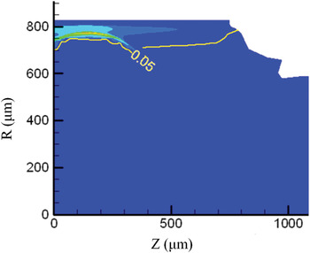
Fig. 11. (Color online) The X-ray emission intensity map and the contour line of ρ = 0.05 g/cm3 at 1.7 ns, with f e = 0.05.

Fig. 12. (Color online) The postprocessed x-ray flux spectrum along the lines at 0°and 20° from the Hohlraum axis through LEH at 1.7 ns, with f e = 0.05.
6. THE EFFECT OF GAS FILLING ON THE WALL PLASMA EXPANSION
To hold back the wall plasma expansion and to ensure that the laser beams propagate to positions near the hohlraum wall, a gas-filled hohlraum is usually used in inertial fusion study. In the experiments done by Huser et al. (Reference Huser, Courtois and Monteil2009) the authors also measured the wall and laser spot motion in a propane-filled hohlraum. In this section, we take f e as 0.07 and compare our simulations with the observations (Huser et al., Reference Huser, Courtois and Monteil2009).
In Figure 13, we present the LARED-H simulations of the temporal r freeO-band, r freeN-band, and r freeM-band in the gas-filled hohlraum and compare them with the experimental results and the FCI2 simulations. For comparison, the simulations of the empty hohlraum are also presented. As shown, from the LARED-H simulations, the wall plasma expansion in the gas-filled hohlraum is much slower than that in the empty hohlraum. Obviously, the LARED-H simulations agree well with the experiments for all three bands when it is shorter than 2 ns, at which the main laser pulse falls around to its half maximum. However, there is some disagreement after 2.3 ns when the main pulse falls rapidly, especially for the N-band and the M-band. From Figure 13, compared to the experimental results and the FCI2 simulations, the N-band emission region after 2.3 ns moves much slower while the M-band moves much faster from the LARED-H.

Fig. 13. (Color online) Comparisons of the temporal r freeO-band (a), r freeN-band (b), and r freeM-band (c) in the gas-filled hohlraum at f e = 0.07 with those from the experimental observations (with black square) and the simulations from FCI2 (with red circle). The LARED-H results for the empty hohlraum are also presented for comparison.
In Figure 14, we compare the simulated temporal relative displacements z 1 at f e = 0.07 with the experimental observations for the gas-filled hohlraum. As shown, the simulations from LARED-H agree with the observations in general, but there are some differences in detail. From the experiments, v I is almost the same, around 40 µm/ns, for whole observation time. However, from the LARED-H simulations, z I has little change within the first 1.5 ns before the main laser pulse reaches its peak, then z I moves with 43 µm/ns between 1.5 ns and 1.8 ns, and with 98 µm/ns after 1.8 ns when the laser pulse falls rapidly.

Fig. 14. (Color online) Comparisons of the simulated temporal relative displacements z I at f e = 0.07 with the experimental observations for the gas-filled hohlraum. Here, v I in blue is obtained from simulations, in black are observed from experiments (Huser et al., Reference Huser, Courtois and Monteil2009) for the laser beams injected at 59°.
SUMMARY
We have studied the influence of f e on hohlraum plasmas by using the LARED-H simulations and proposed a method to experimentally determine f e via the motion of the M-band emission region in Au hohlraum. We have simulated the wall and laser spot motion experiments done by Huser et al. (Reference Huser, Courtois and Monteil2009) by taking different f e. From our simulations, the limited free streaming flux may dominate the heat conduction in the regions with steep temperature gradient, which are important X-ray emission regions. As a result of our study, the motion of the M-band emission region is sensitive to the f e when the limited free streaming flux dominates the heat conduction of the wall plasma expansion region, and one can determine f e via the motion of the M-band emission region.
In general, the LARED-H simulations agree well with the experimental results when f e is taken as 0.07 for both empty hohlraum and gas-filled hohlraum used in Huser's (Reference Huser, Courtois and Monteil2009) experiments. However, there are also some remarkable deviations from the observations, such as the motion of the N-band emissions in the overcritical region and the emission behaviors after 2.3 ns in both empty and gas-filled hohlraums. It is possible that we may have some problems in simulating the hohlraums when laser pulse falls rapidly and hohlraum becomes cold. To understand the disagreements between the simulations and the observations, we will have an experiment for measuring the motion of X-ray emissions on the SG-III prototype laser facility in near future.
ACKNOWLEDGMENT
This work was supported by the National Natural Science Foundation of China, Grant No. 11105014.


