


Introduction
In the last few years, laser-driven proton acceleration (LDPA) has become a growing field of research. The advent of high-power lasers (Dunne, Reference Dunne2006), which can produce accelerated bunches of particles (mainly protons and electrons), has attracted a strong interest in both the conventional and laser-plasma accelerator community. Compared to conventional accelerator machines, laser-driven particle accelerators have the advantage of potentially allowing more compact facilities due to the possibility of reaching accelerating fields in the order of TV/m, up to three orders of magnitude higher than what is typically obtained with radio frequency (RF)-based technology. In the case of LDPA, the target normal sheath acceleration (TNSA) is considered to be one of the most employed and reliable acceleration techniques (Wilks et al., Reference Wilks, Kruer, Tabak and Langdon1992). This scheme implements thin solid foils (with a thickness ranging from a few tens of nm up to a few tens of μm) that are irradiated with an ultra-intense (I > 1018 W/cm2), short laser pulse (i.e., with a duration from a fs to ps), allowing to accelerate proton beams to energies of up to tens of MeV (Macchi, Reference Macchi2017).
These laser-generated proton beams have unique characteristics, such as high charge (1013 particles/shot), high laminarity at the source, short bunch duration (ps at the source), and a high peak current (kA at the source). These characteristics make them desirable candidates for several applications that require one or more of the mentioned properties, such as biomedicine (tumor treatment, PET, radiography) (Bulanov et al., Reference Bulanov, Esirkepov, Khoroshkov, Kuznetsov and Pegoraro2002; Malka et al., Reference Malka, Fritzler, Lefebvre, d'Humières, Régis, Grillon, Albaret, Meyroneinc, Chambaret, Antonetti and Hulin2004), warm dense matter (Patel et al., Reference Patel, Mackinnon, Key, Cowan, Foord, Allen, Price, Ruhl, Springer and Stephens2003; Antici et al., Reference Antici, Fuchs, Atzeni, Benuzzi, Brambrink, Esposito, Koenig, Ravasio, Schreiber, Schiavi and Audebert2006; Bulanov et al., Reference Bulanov, Bychenkov, Chvykov, Kalinchenko, Litzenberg, Matsuoka, Thomas, Willingale, Yanovsky, Krushelnick and Maksimchuk2010; Mancic et al., Reference Mancic, Robiche, Antici, Audebert, Blancard, Combis, Dorchies, Faussurier, Fourmaux, Harmande, Kodama, Lancia, Mazevet, Nakatsutsumi, Peyrussee, Recoules, Renaudin, Shepherd and Fuchs2010), hybrid acceleration schemes (Antici et al., Reference Antici, Fazi, Lombardi, Migliorati, Palumbo, Audebert and Fuchs2008; Scisciò et al., Reference Scisciò, Migliorati, Palumbo and Antici2018) and material science (Dromey et al., Reference Dromey, Coughlan, Senje, Taylor, Kuschel, Villagomez-Bernabe, Stefanuik, Nersisyan, Stella, Kohanoff, Borghesi, Currell, Riley, Jung, Wahlström, Lewis and Zepf2016; Barberio et al., Reference Barberio, Scisciò, Vallières, Veltri, Morabito and Antici2017a, Reference Barberio, Scisciò, Vallières, Cardelli, Chen, Famulari, Gangolf, Revet, Schiavi, Senzacqua and Antici2018a, Reference Barberio, Vallières, Scisciò, Kolhatkar, Ruediger and Antici2018b). Recently, the use of laser-accelerated proton beams as diagnostic for chemical analysis of cultural heritage (CH) artifacts has been investigated (Barberio et al., Reference Barberio, Veltri, Scisciò and Antici2017b; Barberio and Antici, Reference Barberio and Antici2019; Passoni et al., Reference Passoni, Fedeli and Mirani2019). The main challenge in this field is to collect as much information as possible regarding the chemical (Bertrand et al., Reference Bertrand, Schöeder, Anglos, Breese, Janssens, Moini and Simon2015; Santos et al., Reference Santos, Pappalardo, Catalano, Orlando and Romano2016) and morphological (Schreiner et al., Reference Schreiner, Melcher and Uhlir2007) state of the surface and the bulk of the samples (ceramics, paintings, bronze, etc.) while preventing any possible damage (Zucchiatti and Agulló-Lopez, Reference Zucchiatti and Agulló-Lopez2012; Calligaro et al., Reference Calligaro, Gonzalez and Pichon2015; Lazic et al., Reference Lazic, Vadrucci, Fantoni, Chiari, Mazzinghi and Gorghinian2018) as well as find the best way for their conservation and restoration without any esthetical aspect modification. The particle-induced X-ray emission (PIXE) technique, using protons as source, is performed in facilities such as the Accélérateur Grand Louvre d'analyse élémentaire (AGLAE) (Menu et al., Reference Menu, Calligaro, Salomon, Amsel and Moulin1990; Radepont et al., Reference Radepont, Lemasson, Pichon, Moignard and Pacheco2018), located at the French Louvre laboratory – (C2RMF) (Zucchiatti and Redondo-Cubero, Reference Zucchiatti and Redondo-Cubero2014), the AIFIRA facility at Centre d'Etudes Nucléaires Bordeaux-Gradignan (CENBG) (Barberet et al., Reference Barberet, Incerti, Andersson, Delalee, Serani and Moretto2009; Sorieul et al., Reference Sorieul, Alfaurt, Daudin, Serani and Moretto2014) and Instituto Nazionale di Fisica Nucleare–LAboratorio di tecniche nucleari per i BEni Culturali (INFN–LABEC) laboratory in Florence (Italy) (Giuntini et al., Reference Giuntini, Massi and Calusi2007; Ezeh et al., Reference Ezeh, Obioh, Asubiojo, Chiari, Nava, Calzolai, Lucarelli and Nuviadenu2015; Re et al., Reference Re, Angelici, Giudice, Corsi, Allegretti, Biondi, Gariani, Calusi, Gelli, Giuntini, Massi, Taccetti, La Torre, Rigato and Pratesi2015). In these laboratories, conventional electrostatic accelerators (such as Van der Graff tandems or Pellatron types) (Mandò et al., Reference Mandò, Fedi and Grassi2011) generate proton bunches with energies that range from 1 to 5 MeV, a beam current from few pA to nA (Chiari et al., Reference Chiari, Migliori and Mandò2002), a beam charge of the order of nC (Pichon et al., Reference Pichon, Calligaro, Lemasson, Moignard and Pacheco2015). These proton beams irradiate the material samples (ceramics, paintings, bronze, etc.) and excite the emission of X-ray photons. The generated X-ray radiation can be measured with energy-dispersive devices (Bertrand et al., Reference Bertrand, Schöeder, Anglos, Breese, Janssens, Moini and Simon2015) and the retrieved energy spectrum provides information about the chemical components and their quantity present in the bulk of the analyzed samples.
The results reported in Barberio et al. (Reference Barberio, Veltri, Scisciò and Antici2017b) catalyzed the possibility of using a laser-driven proton source for PIXE spectroscopy as an alternative to conventional machines, implementing a “laser-driven PIXE”. Barberio et al. irradiated a silver sample with a laser-accelerated proton beam and were able to retrieve the chemical composition of the target with a single shot. They were able to demonstrate that the damage induced by the laser-accelerated protons was the same (if not lower) than what induced using conventional PIXE. That the short, but intense proton beam achievable using laser-driven PIXE could potentially have a positive impact on the damage induced on the artifact during the time of analysis is still under investigation.
Using a laser-driven proton source also has the advantage of an improved compactness of the acceleration section, compared to large conventional facilities such as NEW AGLAE (2 × 30 m2) (Pichon et al., Reference Pichon, Calligaro, Lemasson, Moignard and Pacheco2015) and INFN-LABEC (40 × 15 m2) (Grassi et al., Reference Grassi, Migliori, Mandò and Calvo del Castillo2005). Using laser-PIXE, it is possible to scan larger volumes of the artworks with a single shot covering surfaces up to cm2, while the final spot sizes that are typical of conventional accelerators go from a few μm (~1–2 µm) up to 500 µm. The broad energy range of laser-driven proton sources permits the “tuning” of the beam energy in a broad range from few KeV to tens of MeV, potentially allowing a “layer by layer” analysis of the irradiated bulk material.
The total time for performing a full PIXE analysis depending on the allowable current on the sample and the required photons for having a reliable Signal-to-Noise ratio on the X-ray detector. Our technique is able to scan a larger surface and – depending on the energy spread – perform volumetric analysis, compared to conventional accelerators. In applications where this is useful, our technique can be quicker than conventional accelerators; however, when the useable current is limited, the energy spread needs to be low and the spot size is the same, the analysis time stays the same since this depends on the global flux.
Currently, the high beam divergence (few tens of degrees at the source) and the high energy spread (up to 100%) of laser-generated protons limit the efficiency of energy-selected beams for applications, including laser-PIXE. To overcome these issues, novel alternative acceleration techniques/regimes (Antici et al., Reference Antici, Boella, Chen, Andrews, Barberio, Böker, Cardelli, Feugeas, Glesser, Nicolaï, Romagnani, Scisciò, Starodubtsev, Willi, Kieffer, Tikhonchuk, Pépin, Silva, d’ Humières and Fuchs2017; Macchi, Reference Macchi2017; Sharma, Reference Sharma2018) and the use of sophisticated targets (Barberio et al., Reference Barberio, Scisciò, Veltri and Antici2016; Sharma et al., Reference Sharma, Tibai, Hebling and Fülöp2018) have been studied theoretically and experimentally (Kraft et al., Reference Kraft, Obst, Metzkes-Ng, Schlenvoigt, Zeil, Michaux, Chatain, Perin, Chen and Fuchs2018; Morrison et al., Reference Morrison, Feister, Frische, Austin, Ngirmang, Murphy, Orban, Chowdhury and Roquemore2018) with the aim of better controlling the acceleration mechanism and improving the proton beam yield.
Alternatively, to optimizing directly the laser-driven proton source, there have been different proposals manipulating the TNSA-generated proton beams downstream the laser–plasma interaction point using conventional accelerator devices, implementing so-called hybrid beamlines or post acceleration schemes. Numerous research groups have studied these schemes, in view of potential applications: using a RF cavity (Nakamura et al., Reference Nakamura, Ikegami, Iwashita, Shirai, Tongu, Souda, Daido, Mori, Kado, Sagisaka, Ogura, Nishiuchi, Orimo, Hayashi, Yogo, Pirozhkov, Bulanov, Esirkepov, Nagashima, Kimura, Tajima, Takeuchi, Fukumi, Li and Noda2007), permanent quadrupoles magnets (PMQ) (Schollmeier et al., Reference Schollmeier, Becker, Geißel, Flippo, Blažević, Gaillard, Gautier, Grüner, Harres, Kimmel, Nürnberg, Rambo, Schramm, Schreiber, Schütrumpf, Schwarz, Tahir, Atherton, Habs, Hegelich and Roth2008; Ter-Avetisyan et al., Reference Ter-Avetisyan, Schnürer, Polster, Nickles and Sandner2008; Nishiuchi et al., Reference Nishiuchi, Daito, Ikegami, Daido, Mori, Orimo, Ogura, Sagisaka, Yogo, Pirozhkov, Sugiyama, Kiriyama, Okada, Kanazawa, Kondo, Shimomura, Tanoue, Nakai, Sasao, Wakai, Sakaki, Bolton, Choi, Sung, Lee, Oishi, Fujii, Nemoto, Souda, Noda, Iseki and Yoshiyuki2009) a compact travelling wave accelerator (Kar et al., Reference Kar, Ahmed, Prasad, Cerchez, Brauckmann, Aurand, Cantono, Hadjisolomou, Lewis, Macchi, Nersisyan, Robinson, Schroer, Swantusch, Zepf, Willi and Borghesi2016), and adapting the beamlines to more specific applications, for example, the medical field (Busold et al., Reference Busold, Schumacher, Deppert, Brabetz, Frydrych, Kroll, Joost, Al-Omari, Blažević, Zielbauer, Hofmann, Bagnoud, Cowan and Roth2013, Reference Busold, Schumacher, Deppert, Brabetz, Kroll, Blažević, Bagnoud and Roth2014; Masood et al., Reference Masood, Bussmann, Cowan, Enghardt, Karsch, Kroll, Schramm and Pawelke2014; Romano et al., Reference Romano, Schillaci, Cirrone, Cuttone, Scuderi, Allegra, Amato, Amico, Candiano, De Luca, Gallo, Giordanengo, Fanola Guarachi, Korn, Larosa, Leanza, Manna, Marchese, Marchetto, Margarone, Milluzzo, Petringa, Pipek, Pulvirenti, Rizzo, Sacchi, Salamone, Sedita and Vignati2016). In particular, between 2008 and 2011, several groups used a set of PQMs (Ter-Avetisyan et al., Reference Ter-Avetisyan, Schnürer, Polster, Nickles and Sandner2008; Nishiuchi et al., Reference Nishiuchi, Daito, Ikegami, Daido, Mori, Orimo, Ogura, Sagisaka, Yogo, Pirozhkov, Sugiyama, Kiriyama, Okada, Kanazawa, Kondo, Shimomura, Tanoue, Nakai, Sasao, Wakai, Sakaki, Bolton, Choi, Sung, Lee, Oishi, Fujii, Nemoto, Souda, Noda, Iseki and Yoshiyuki2009), that, respectively, focused proton beams in the range of (3.7 ± 0.3) MeV, collected a final bunch of ~108 particles and (2.4 ± 0.1) MeV with ~106 particles. For reducing the energy spread of the protons, passive magnetic chicanes (Chen et al., Reference Chen, Gauthier, Higginson, Dorard, Mangia, Riquier, Atzeni, Marquès and Fuchs2014; Scuderi et al., Reference Scuderi, Bijan Jia, Carpinelli, Cirrone, Cuttone, Korn, Licciardello, Maggiore, Margarone, Pisciotta, Romanob, Schillaci, Stancampiano and Tramontana2014; Scisciò et al., Reference Scisciò, Migliorati, Palumbo and Antici2018) have been employed as energy selectors (ES).
In this work, we aim at optimizing the performance of a laser-driven hybrid beamline and compare it to typical parameters of conventional facilities dedicated to PIXE spectroscopy. The proposed beamline design includes an ES, with similar features as reported in Scisciò et al. (Reference Scisciò, Migliorati, Palumbo and Antici2018), followed by magnetic focusing devices [i.e., Permanent Magnet Quadrupoles (PQM)] in order to vary the final transverse dimensions of the energy-selected beam on the CH sample. The used ES provides the possibility of tuning the beam energy in the range that is typical for the PIXE analysis, that is, 1–5 MeV, reducing the initial energy spread to a final value of ≤10%. The ability to select different energies in a short time allows exploiting the possibility of performing a “layer by layer” analysis of the artifact (Barberio and Antici, Reference Barberio and Antici2019). The reduced energy spread also allows coupling the beam exiting the ES with focusing PQMs for modifying the analyzed surface on the CH sample (the broad energy spread of an unselected beam would lead to unsustainable chromatic effects in the focusing section). The variation of the PMQ's position between the ES and the sample allows tuning the final transverse beam spot size from a fraction of mm2 up to 1–2 cm2. This potentially permits scanning a cm2 area with a few laser shots. We also estimate the final charge of the proton bunch, which needs to be high enough to be comparable to what is obtained on conventional facilities (in the order of nC/shot or a fraction of nC/shot if using a higher-repetition rate laser) (Pichon et al., Reference Pichon, Calligaro, Lemasson, Moignard and Pacheco2015). We study the main parameters of the transport line using beam dynamics simulation codes, namely TRACE3D and TSTEP, that are a standard tool for optimizing accelerator devices (Young, Reference Young1996; Crandall and Rusthoi, Reference Crandall and Rusthoi1997).
The obtained results show that combining our compact hybrid beamline with a multi-Hz laser system allows to perform PIXE spectroscopy with features comparable to what obtained on conventional accelerators based on RF technology, potentially reducing the time of analysis of a larger surface to a few tens of seconds and the dimensions of the entire beamline (to a total length of <1 m).
The paper is organized as follows: We initially describe the methodology for optimizing our proposed hybrid beamline scheme. In the section ‘Analysis of the ES’, we analyze only the ES contribution and performance and we select the best features in terms of energy tunability and energy range. In the section ‘Optimization of the focusing section based on PMQs’, we present a study of the entire hybrid beamlineincluding the focusing elements (i.e., the ES followed by one or two PMQs). We investigate three total length scenarios for our hybrid beamlines. These should fit in a medium/big size vacuum chamber. In LDPA, these have a typical diameter of around 1 m for TW laser systems (Fuchs et al., Reference Fuchs, Sentoku, Karsch, Cobble, Audebert, Kemp, Nikroo, Antici, Brambrink, Blazevic, Campbell, Fernández, Gauthier, Geissel, Hegelich, Pépin, Popescu, Renard-LeGalloudec, Roth, Schreiber, Stephens and Cowan2005) or, in PW facilities, can reach a diameter of 2 m (Barberio et al., Reference Barberio, Veltri, Scisciò and Antici2017b). Our three scenarios are: (1) the ES coupled to one quadrupole aiming at a total length of 80 cm; (2) the ES coupled to one quadrupole aiming at a compact design of 50 cm total length; (3) the ES coupled to two PMQs in a FODO configuration. Finally, the conclusions are drawn.
Analysis of the ES
The hybrid beamline that we have optimized for the PIXE analysis is qualitatively represented in Figure 1 and has been studied using the above-mentioned codes TRACE3D and TSTEP.
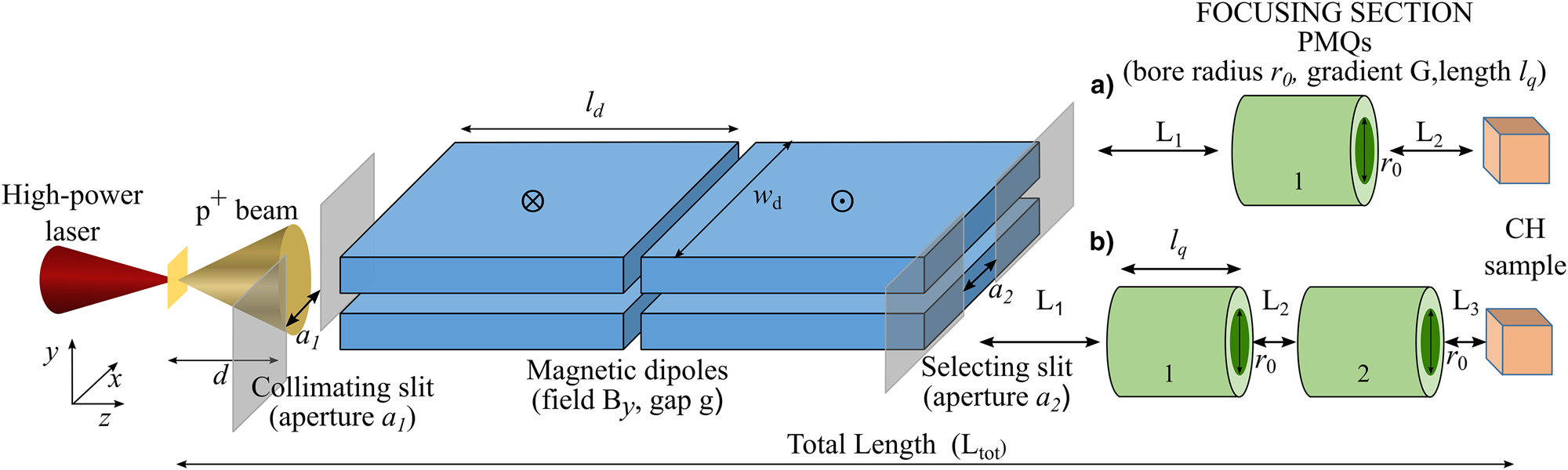
Fig. 1. Qualitative scheme of the hybrid beamline. It is composed of an ES, consisting of two dipoles [both of length l d = 10 cm; width w d = 10 cm; By = 0.92 T (incoming magnetic field for the first dipole and outgoing magnetic field for the second one), gap size of 0.9 cm], a collimating slit (a 1) and the central selecting slit (a 2), followed by one or multiple PMQs. The first slit, with distance from the source d and aperture a 1 can be varied for collimating the beam, i.e. reducing the initial divergence. The particles are then displaced transversely (along the x-axis) with respect to the direction of propagation (z) by the bending dipoles according to their velocity. The aperture a 2 of the selecting slit provides the energy selection and reduces the final energy spread of the protons. The PMQ parameters [with length l q, bore radius r 0 (internal diameter) and the gradient G] are optimized in order to focus/defocus the final transverse spot size on the irradiated sample. We consider as possible focusing sections two scenarios: ES followed by one PMQ (a) and ES followed by two PMQs (b). The total distance L tot is maximum 80 cm and the drifts are, respectively, L 1 and L 2 in the case (a) and L 1, L 2, L 3 in case (b). By varying the values of distances L 1, L 2 or L 1, L 2, L 3, the transverse dimensions of the final beam can be tuned.
At first, we have studied the ES that accounts for reducing the energy spread of the proton bunch. We have adopted a similar methodology as reported in Scisciò et al. (Reference Scisciò, Migliorati, Palumbo and Antici2018).
Commonly, an ES is implemented as follows: a magnetic dipole chicane with one entrance slit and one selecting slit (see Fig. 1) (Chen et al., Reference Chen, Gauthier, Higginson, Dorard, Mangia, Riquier, Atzeni, Marquès and Fuchs2014; Scuderi et al., Reference Scuderi, Bijan Jia, Carpinelli, Cirrone, Cuttone, Korn, Licciardello, Maggiore, Margarone, Pisciotta, Romanob, Schillaci, Stancampiano and Tramontana2014; Scisciò et al., Reference Scisciò, Migliorati, Palumbo and Antici2018). The entrance slit (a 1) reduces the initial divergence of the beam that enters the dipoles. The particles (accelerated along z) are then dispersed transversely along x by a distance that depends on their velocity. The aperture of the second slit (a 2), which is movable on the dispersion plane along the x-axis, accounts for the energy selection of the protons. After the central selecting slit (a 2) – see Figure 1 – two additional dipoles realign the selected beam along the initial propagation axis. We limit our beamline design to using only two dipoles. Adding further two dipoles would allow bending the beam back to its original trajectory axis. However, the characteristics of the beam using 4 dipoles are not as competitive as using only 2 dipoles. For the applications, it is not relevant to keep the beam on its original propagation axis. We therefore limit the present study to only 2 dipoles.
The main dipole parameters, as reported in Figure 1, are a length of l d = 10 cm, a width of w d = 10 cm, a vertical gap of g = 0.9 cm (i.e., the dipole gap in y-direction), and magnetic field B y = 0.92 T (incoming magnetic field for the first dipole and outgoing magnetic field for the second one). These parameters are similar to what is reported in Scisciò et al. (Reference Scisciò, Migliorati, Palumbo and Antici2018), where a selector in the energy range 2–20 MeV has been optimized and has been adapted to our range of 1–5 MeV. For studying the energy selection process, we simulate an initial proton beam having a uniform energy distribution with energy spread  ${{{\rm \Delta} E} / {E_0}}$ of 100% (the black spectrum of Fig. 2) and evaluate the final energy spread after the selection slit (the colored spectra of Fig. 2). The first selector parameter that we analyze is the initial beam divergence: we aim at indicating a maximum initial divergence that is compatible with the final beam parameters that are required for the PIXE analysis (Grassi et al., Reference Grassi, Migliori, Mandò and Calvo del Castillo2005; Pichon et al., Reference Pichon, Calligaro, Lemasson, Moignard and Pacheco2015).

Fig. 2. Final energy spread as function of the initial divergence, for the case of 1 MeV (a), 3 MeV (b), and 5 MeV (c), at the exit of the selector. The initial divergence has the values: 3 mrad (red color), 5 mrad (green color), 7 mrad (light blue color), 10 mrad (magenta color). The dark black curve represents the unselected beam at the entrance of the selector. (d) Final energy spectra in the case of 1, 3, and 5 MeV beams, selected using 5 mrad and a 2 = 1000 μm (1 MeV beam), and 3 mrad and a 2 = 500 μm (3 and 5 MeV beams).
The initial divergence is determined by the aperture a 1 of the first slit and its distance d from the laser–plasma source. For example, an aperture a 1 = 500 μm and an initial divergence of 3 mrad correspond to a distance between the laser proton source and the entrance of the ES of d = 8 cm. We vary the initial divergence from a minimum of 3 mrad up to 10 mrad (half angle) for the three energy cases 1, 3, and 5 MeV. The final achieved energy spread is reported in Figure 2, where it is shown that the increase in the initial divergence leads to an increase in the final energy spread. The simulations show that this increase starts to be particularly significant for a divergence ≥7 mrad for the cases of 3 and 5 MeV. When selecting 1 MeV protons (Fig. 2a), the FWHM energy spread ranges from 3% (for 3 mrad initial divergence) to 11% (10 mrad initial divergence). For the cases of 3 and 5 MeV (Fig. 2b and 2c), an initial divergence of 10 mrad leads to a final energy spread of 23 and 30%, respectively. This is an increase of a factor three with respect to the case of an initial divergence of 3 mrad (8 and 10% final energy spread, for 3 and 5 MeV, respectively).
This is due, as reported in Chen et al. (Reference Chen, Gauthier, Higginson, Dorard, Mangia, Riquier, Atzeni, Marquès and Fuchs2014) and Scisciò et al. (Reference Scisciò, Migliorati, Palumbo and Antici2018), to the natural intrinsic divergence and emittance growth of the proton beam at the source (Migliorati et al., Reference Migliorati, Bacci, Benedetti, Chiadroni, Ferrario, Mostacci, Palumbo, Rossi, Serafini and Antici2013) which adds further deviation from the normal trajectory induced by the magnetic field of the dipoles.
According to these results, we define our optimal initial divergence as a compromise between the final energy spread, which should be  $\le \!\!10\%$, and the number of particles transmitted through the slit, which obviously decrease in case of smaller apertures. Moreover, this energy spread range is acceptable, considering that the energy interval 1–5 MeV allows to investigate the first few μm of CH samples. For the initial slit at a distance d = 8 cm from the laser–plasma source in the case of 1 MeV, we use an aperture of a 1 = 800 μm, obtaining a divergence of 5 mrad. Similarly, for both 3 and 5 MeV cases, we choose an aperture of a 1 = 500 μm leading to an initial divergence of 3 mrad.
We also analyze the aperture a 2 of the selecting slit that is needed for the final energy selection and allows obtaining the narrow energy spread. The width of the aperture should be a compromise between the desired final energy spread and the number of transmitted particles that is required in order to have a final charge that is comparable to what is implemented on conventional PIXE facilities. A smaller value of a 2 leads to a reduction of the final number of particles that is transmitted through the selector. For selecting lower energy particles, which experience a larger displacement by the dipole field, a larger aperture is allowed in order to obtain a final energy spread  $\le \!\!10\%$. Therefore, we choose as a compromise an aperture of the central slit of a 2 = 1000 μm for selecting a 1 MeV beam and an aperture of a 2 = 500 μm for the cases of 3 and 5 MeV. These three choices of different energies are the most employed energies when using PIXE applications (Grassi et al., Reference Grassi, Migliori, Mandò and Calvo del Castillo2005) and allow obtaining a FWHM final energy spread ≤10% in the energy range of our interest. In Figure 2d, we report the final energy spectra of 1, 3, and 5 MeV beams, selected using these optimized parameters of initial divergence, that are, the distance d, slit width a 1 and slit width a 2.
For a selected central energy (1–3–5 MeV), we obtain the respective selected final energy range (Fig. 2d). We define the transmission efficiency of the beamline ηBL as the ratio between the number of particles that reach the CH sample (final beam) and the number of particles that pass through the initial slit of the ES, in the same final selected energy range. For the central energy 1 MeV, we obtain the value  ${{\rm {\eta}}} _{\rm {BL}\; \;} \simeq 12\%$, while for the central energies 3 and 5 MeV, the value of ηBL is ≃9%. With ηBL, we do not take into account the losses induced by the collimation slit (with width a 1). These initial losses strongly depend on the characteristics of the laser–plasma interaction that generates the protons, such as the beam energy-divergence distribution at the source. Since we do not focus our study on a specific case of laser–plasma interaction conditions, we estimate these losses with ηS from the solid angle of the collimation slit's aperture. The horizontal divergence at the source is reduced by the initial collimating slit to a value of 3 mrad (for the cases of 3 and 5 MeV, 5 mrad for the case of 1 MeV). In the vertical plane, the divergence is only limited by the vertical aperture of the dipoles (~1 cm), corresponding to a half angle of 56 mrad. Taking into account that the mean divergence of a TNSA beam at the source typically is about 15° half angle (Mancic et al., Reference Mancic, Robiche, Antici, Audebert, Blancard, Combis, Dorchies, Faussurier, Fourmaux, Harmande, Kodama, Lancia, Mazevet, Nakatsutsumi, Peyrussee, Recoules, Renaudin, Shepherd and Fuchs2010; Green et al., Reference Green, Robinson, Booth, Carroll, Dance, Gray, MacLellan, McKenna, Murphy, Rusby and Wilson2014), corresponding to a solid angle of around 0.21 steradiant, the collimation slit induces a loss of
  ${{\rm {\eta}}} _{\rm S} = 0.31\%$ for the energy cases of 3 and 5 MeV. This value is higher for the case of 1 MeV protons where we obtain
  ${{\rm {\eta}}} _{\rm S}\; = 0.50\%$, due to the initial horizontal collimation of 5 mrad that is achieved with a wider slit aperture (a 1 = 800 μm). The final total transport efficiency (i.e., from the source to the end of the line) is ηT = ηS · ηBL and we obtain
  ${{\rm {\eta}}} _{\rm T} = 0.059\,\%$ for the 1 MeV beam and
  ${{\rm {\eta}}} _{\rm T} = 0.028\,\%$ and for the 3 and 5 MeV beams. This efficiency could be improved using a focusing section before entering the first dipole.
With these values, it is possible to estimate the bunch charge that is delivered to the sample for each mean energy within one single laser shot. From a typical TNSA proton spectrum (Fuchs et al., Reference Fuchs, Sentoku, Karsch, Cobble, Audebert, Kemp, Nikroo, Antici, Brambrink, Blazevic, Campbell, Fernández, Gauthier, Geissel, Hegelich, Pépin, Popescu, Renard-LeGalloudec, Roth, Schreiber, Stephens and Cowan2005; Fourmaux et al., Reference Fourmaux, Buffechoux, Albertazzi, Capelli, Lévy, Gnedyuk, Lecherbourg, Lassonde, Payeur, Antici, Pépin, Marjoribanks, Fuchs and Kieffer2013; Green et al., Reference Green, Robinson, Booth, Carroll, Dance, Gray, MacLellan, McKenna, Murphy, Rusby and Wilson2014), obtained using a TW-class laser system with a repetition rate in the range 1–10 Hz, we can set values for the initial charge at the source. Taking as benchmark for the number of particles, a typical proton spectrum as produced by a high-power short-pulse laser of new generation (Green et al., Reference Green, Robinson, Booth, Carroll, Dance, Gray, MacLellan, McKenna, Murphy, Rusby and Wilson2014), and considering the central energies of 1, 3, and 5 MeV with a final energy spread of, respectively, 6, 8, and 10% we obtain about 5 · 1011, 5 · 1011, and 1 · 1011 particles per shot, respectively. After all the losses along the line, the final charge on the sample is ~0.05 nC/shot for 1 MeV, ~0.02 nC/shot for 3 MeV, and ~0.004 nC/shot for 5 MeV. A reference value for the total charge that is used in order to retrieve the PIXE signal from a scanned area of the sample is reported in Pichon et al. (Reference Pichon, Calligaro, Lemasson, Moignard and Pacheco2015) where 1.8 nC are used to scan a sub-millimetric area. Coupling our beamline to a 1 Hz high-intense laser system allows cumulating a similar final charge in less than 10 min irradiation for the 1–3–5 MeV beams. These time expositions can be further decreased by a factor 10 using the new upcoming 10 Hz high-intensity laser systems (Kühn et al., Reference Kühn, Dumergue, Kahaly, Mondal, Füle, Csizmadia, Farkas, Major, Várallyay, Cormier, Kalashnikov, Calegari, Devetta, Frassetto, Månsson, Poletto, Stagira, Vozzi, Nisoli, Rudawski, Maclot, Campi, Wikmark, Arnold, Hey, Johnsson, L'Huillier, Lopez-Martens, Haessler, Bocoum, Boehle, Vernier, Iaquaniello, Skantzakis, Papadakis, Kalpouzos, Tzallas, Lépine, Charalambidis, Varjú, Osvay and Sansone2017; Mondal et al., Reference Mondal, Shirozhan, Ahmed, Bocoum, Boehle, Vernier, Haessler, Lopez-Martens, Sylla, Sire, Quéré, Nelissen, Varjú, Charalambidis and Kahaly2018; Roso, Reference Roso2018).
Optimization of the focusing section based on PMQs
This section describes the results obtained from the second set of simulations that are performed in order to investigate the combination of the ES with the focusing/defocusing PMQs. For optimizing our design, we consider two different scenarios. At first, we aim at focusing/defocusing the proton beam using a single quadrupole and for the total length of the beamline (Fig. 1) we consider a case with 50 cm total length (this represents a compact beamline that can be easily adapted to a medium/large vacuum chamber (Fuchs et al., Reference Fuchs, Sentoku, Karsch, Cobble, Audebert, Kemp, Nikroo, Antici, Brambrink, Blazevic, Campbell, Fernández, Gauthier, Geissel, Hegelich, Pépin, Popescu, Renard-LeGalloudec, Roth, Schreiber, Stephens and Cowan2005; Barberio et al., Reference Barberio, Veltri, Scisciò and Antici2017b; Nilsson et al., Reference Nilsson, Andersson, Engström, Lundberg and Hartman2019; Vallières et al., Reference Vallières, Puyuelo-Valdes, Salvadori, Bienvenue, Payeur, d'Humières, Antici, Esarey, Schroeder and Schreiber2019) and a case with 80 cm total length [an extended version where the range of the final spot size of the beam is broader but presumably requires an extension if implemented in a chamber of common dimensions, which can also be desirable for inserting additional diagnostics (Bolton et al., Reference Bolton, Borghesi, Brenner, Carroll, De Martinis, Fiorini, Flacco, Floquet, Fuchs, Gallegos, Giove, Green, Green, Jones, Kirby, McKenna, Neely, Nuesslin, Prasad, Reinhard, Roth, Schrammm, Scott, Ter-Avetisyan, Tolley, Turchettin and Wilkens2014)]. Secondly, we study the case where two quadrupoles are used, in a FODO configuration, in order to focus/defocus the beam. In that case, the total length of the beamline is about 80 cm. The distance between the source and the sample has a fixed value for each scenario that we study: in this way, we manipulate the proton beam (i.e., change the selected energy or vary the final spot size) without the necessity of displacing the sample.
The key design parameters of the PQMs are the bore radius r 0, the magnetic field gradient G, and the magnetic length l q. The maximum achievable gradient is related to the magnetic field B 0 on the quadrupole's pole tip and the bore radius, as G = B 0/r 0. We choose for our beamline design a PMQ length of l q = 4.5 cm and a bore radius of r 0 = 1 cm. These parameters can be easily obtained with the existing permanent magnet technology (Halbach and Holsinger, Reference Halbach and Holsinger1976; Eichner et al., Reference Eichner, Grüner, Becker, Fuchs, Habs, Weingartner, Schramm, Backe, Kunz and Lauth2007; Nirkko et al., Reference Nirkko, Braccini, Ereditato, Kreslo, Scampoli and Weber2013; Marteau et al., Reference Marteau, Ghaith, N'Gotta, Benabderrahmane, Valléau, Kitegi, Loulergue, Vétéran, Sebdaoui, André, Le Bec, Chavanne, Vallerand, Oumbarek, Cosson, Forest, Jivkov, Lancelot and Couprie2017) and allow us to keep the dimensions of the beamline compact. Using rare-earth materials, these features allow obtaining a value of B 0 in the range of hundreds of mT (Eichner et al., Reference Eichner, Grüner, Becker, Fuchs, Habs, Weingartner, Schramm, Backe, Kunz and Lauth2007; Nirkko et al., Reference Nirkko, Braccini, Ereditato, Kreslo, Scampoli and Weber2013) and a field gradient in the order of several tens of T/m.
Focusing section based on a single quadrupole
We first perform TRACE3D simulations, which evaluate the beam envelope along the line, in order to optimize the focusing section. The obtained results are then compared and validated with TSTEP simulations, performed in the same conditions (i.e., same PMQ parameters, same distances between the transport elements). TRACE3D provides an optimization routine that indicates the optimal parameters of the line based on matching conditions of the beam Twiss parameters (α, β, γ) between two different positions of the transport line (in our case between the exit of the ES and the irradiated sample). The aim is to optimize the position of the quadrupole for obtaining a variable final beam transverse dimension on the sample, ranging from a few mm up to the order of cm.
For the three mean energies of our interest 1, 3, and 5 MeV, the simulated gradient of the quadrupoles is set at G = 60 T/m (with magnetic length l q = 4.5 cm). This value is obtained from preliminary optimizations with TRACE3D where different gradients have been exploited: it is a good compromise for operating at these different energies and it is a compatible value with the typical field intensities of commercial PMQs of this size. The initial values of the Twiss parameters (α, β, γ) are calculated according to the transverse beam geometry at the exit of the ES and represent the initial beam conditions for the TRACE3D simulations. The horizontal (in x-direction) dimension of the beam is determined by the aperture a 2 of the selecting slit of the ES [1 mm for 1 MeV, 500 µm for 3 (Fig. 3a) and 5 MeV], while the vertical dimension (along y) depends by the dipoles’ s gap G (the vertical aperture is of 0.9 cm). These parameters are reported in Figure 3b where the phase space of the protons at the end of the ES is plotted for the case of 3 MeV beam energy.

Fig. 3. (a) Scheme of the simulated beamline. The numbers in the table indicate the values of L 1 and L 2 for the corresponding colored plot in (c) and (d). (b) Initial phase space, as obtained at the exit of the selector that is used for calculating the input Twiss parameters of the TRACE3D simulations. (c) and (d) Final phase space obtained with the TRACE3D optimized distances L 1 and L 2 for a focused and defocused beam, respectively.
For calculating the optimal position of the PMQ between the selector and the sample, we set the drift spaces before and after the quadrupole location, indicated in Figure 3a with L 1 and L 2, as free parameters. We define conditions on the final Twiss parameters on the y-coordinate with the values αy = 0 and βy = 0.008 m for obtaining a collimated beam and a decreased final spot size (small irradiated area on the sample). Then we repeat the optimization routine with the values αy = 28 and βy = 1.4804 m for obtaining a defocused beam, that is, a final spot size with increased dimensions (large irradiated area on the sample). The numerical values of αy, βy reported and respectively associated with the smallest and largest irradiated areas on the sample, are calculated, through Matlab routines, from TSTEP data simulations and are fixed and used as references for the optimization runs. The total distance between the source and the final longitudinal position (i.e., the position where the irradiated sample is placed) is fixed at 80 cm. The matching routine retrieves, for both, the smallest and the largest spot size, the optimized values of L 1 and L 2. In Figure 3c and 3d, we report, as an example among the three possible energy cases, the final transverse phase space obtained with the TRACE3D optimization routine and refined with a particle tracking simulation with TSTEP, of a beam with a mean energy of 3 MeV passing through a y-focusing PMQ that has the following optimized distances: L 1 = 25.7 cm, L 2 = 9.8 cm for the focused, small final spot size and L 1 = 3 cm, L 2 = 32.5 cm for the defocused, large final spot size.
These optimized parameters of the beamline are simulated again with the particle tracking code TSTEP that computes the final transverse spot of the beam from a realistic proton distribution, tracking the trajectory of the single macroparticles. We repeat the process for the energies 1, 3, and 5 MeV: the results are shown in Figure 4. The final energy spread is not altered by the addition of one (or multiple, as discussed later) PMQ: the results of Figure 2 remain unchanged. The value of ηBL does not change when adding these newly optimized PMQs: no additional particle losses are induced and the overall transport efficiencies are the same as calculated in the previous section. From the plots of Figure 4a, one can see that with this configuration it is possible to scan areas of the CH sample with dimensions in the cm2 range, represented in Figure 4b–d with the blue dots. Simply by changing the position of the PMQ and keeping all other parameters unvaried, it is possible to focus the beam (red plot) and achieve a precision on the vertical axis of <1 mm.

Fig. 4. (a) Scheme of the simulated beamline and position of the PMQ, charge, energy, and final transverse spot size dimensions for the analyzed cases. (b)–(d) Final transverse dimensions of the focused (red plot) and defocused (blue plot) proton beam for the cases of 1, 3, and 5 MeV, respectively. These spot sizes are obtained with a single PMQ after the selector, having a length of 4.5 cm and a magnetic field gradient of 60 T/m. The entire beamline (from the proton source to the CH sample) has a length of 80 cm.
As an alternative to the 80 cm long beamline, we also study the possibility of reducing the total length in order to design a line that can possibly fit in a medium size experimental chamber. We aim at obtaining a variable final spot size in the same range as for the longer beamline case (from the mm to the cm range) within a total distance of about 50 cm from the laser–plasma source. We repeat the same procedure as before: the TRACE3D matching algorithm provides indications for the optimized position (for small/large final spot size) and gradient of the PMQ. These values are then validated by additional TSTEP simulations. The optimized design for the case of a 50 cm long beamline is reported in Figure 5a, where the layout is shown and the final beam spot sizes for the energy cases 1–3–5 MeV are plotted. In Figure 5b–d, the smallest achievable spot size as identified by the red dots and the largest achievable spot size (blue dots) are shown.

Fig. 5. (a) Scheme of the simulated beamline and position of the PMQ, charge, energy, and final transverse spot size dimensions for the analyzed cases. (b)–(d) Final transverse dimensions of the focused (red plot) and defocused (blue plot) proton beam for the cases of 1, 3, and 5 MeV, respectively. These spot sizes are obtained with a single PMQ after the selector, having a length of 4.5 cm and a magnetic field gradient of 100 T/m. The entire beamline (from the proton source to the CH sample) has a length of 50 cm.
As before, the used PMQ has a length of l q = 4.5 cm and a bore radius r 0 = 1 cm. The gradient needs to be increased to G = 100 T/m. This allows to shorten the focal distance and obtain both the biggest and the smallest final transverse spot sizes on the CH sample. As shown in Figure 5b–d, this beamline allows to enlarge the final vertical (y-axis) transverse dimension up to about 1 cm for all the analyzed energies. Final spot sizes in the sub-millimetric range are also obtainable for all mean energies by varying the position of the PMQ between the exit of the ES and the end of transport line. In the 3 MeV case, by placing the PMQ 5.3 cm after the exit of the selector, a final vertical dimension of ~0.4 mm is obtained (see Fig. 5c). With this compact scheme, the final energy spread is the same as what is reported in Figure 2 and the transport efficiency is not influenced by the focusing section: as before, we have  ${{\rm {\eta}}} _{\rm T} = 0.028\,\%$ (3 and 5 MeV) and
  ${{\rm {\eta}}} _{\rm T} = 0.059\,\%$ (1 MeV).
ES followed by two PQMs
As an alternative to a focusing section with only one PMQ, we also study the possibility of implementing two PQMs after the ES. We use the same methodology as for the beamlines analyzed before. In the three energy cases reported in Figure 6, the two PMQs are in a FODO configuration where the first quadrupole (closer to the selector) focuses in y and the second focuses in x. We firstly perform a series of preliminary TRACE3D simulations in order to find a viable gradient compromise for all three energy cases: the optimized parameters of the previous configuration, that are l q = 4.5 cm, G = 60 T/m, and r 0 = 1 cm for both PMQs, are suitable for the FODO scheme. The additional PMQ, if carefully optimized, allows to obtain more symmetric spot sizes (in x and y) compared to the previous cases with a single PMQ where asymmetric, elongated final spots are obtained.

Fig. 6. (a) Scheme of the simulated beamline and position of the PMQ, charge, energy, and final transverse spot size dimensions for the analyzed cases. (b)–(d) Final transverse dimensions of the focused (red plot) and defocused (blue plot) proton beam for the cases of 1, 3, and 5 MeV, respectively. These spot sizes are obtained with a pair of PMQs in a FODO configuration. They have a length of 4.5 cm and a magnetic field gradient of 60 T/m. The first PMQ focuses in y-direction, the second PMQ focuses in x-direction. The entire beamline (from the proton source to the CH sample) has a length of ~80 cm.
After having optimized the PMQ gradients, we have performed additional TRACE3D simulations in order to optimize their position with respect to the exit of the ES: similarly, as before, our goal is to obtain an optimized spacing of the PMQs for a focused (small) and defocused (large) spot size on the irradiated sample, by keeping a fixed distance between the proton source and the sample. The optimization regarding the gradients and the positions of the PMQ pairs, provided by TRACE3D simulations, are compared and tested with TSTEP: the particle tracking results allow a further tuning of the spacing and we achieve the final spot sizes for the different energy cases reported in Figure 6. These optimized results allow us to find small/large quasi-symmetric transverse spot sizes with the spacing details that are showed in Figure 6a. The number of transmitted particles keeps unaltered by the addition of one PMQ. The final transverse spot sizes are in the cm2 range when the PMQ spacing is optimized for obtaining a defocused beam (see Fig. 6b–d) where a final spot size of >1 cm2 is obtained for the 1 MeV case and about 0.6 × 0.6 cm for the 5 MeV case. When the spacing is optimized for focusing the beam on the sample, small spot sizes are obtained: we obtain millimetric dimensions on both transverse axes, for all investigated energies (the smallest spot is achieved for the 5 MeV case with ~1 mm on both transverse axis). In this case with a PMQ section implementing a quadrupole pair, the total length of the beamline is of ~80 cm for all energies, that is, the same order of magnitude as the cases with a single PMQ. This allows to fix the position of the irradiated sample with respect to the proton source and the variation of the spot size dimension and energy can be achieved by changing the spacing of the PMQs after the selector. Compared to the scheme with a single PMQ, this beamline has the advantage of producing quasi-symmetric final spot sizes. This can potentially be an advantage for scanning small areas (below 1 mm) on the sample with a more concentrated charge and an improved precision.
We can perform “layer-by-layer” PIXE analysis without resetting the electrostatic accelerator as it is done conventionally (Chiari et al., Reference Chiari, Migliori and Mandò2002; Grassi et al., Reference Grassi, Migliori, Mandò and Calvo del Castillo2005). The overall (i.e., from the proton source to the sample) transmission efficiency is  ${{\rm {\eta}}} _{\rm T} = 0.028\,\%$ for the 3 and 5 MeV beams, while for the case of 1 MeV we obtain
  ${{\rm {\eta}}} _{\rm T} = 0.059\%$. With these values, after taking into account all the losses along the line, it is possible to deliver a final charge on the sample of ~0.05 nC/shot for 1 MeV, ~0.02 nC/shot for 3 MeV, and ~0.004 nC/shot for 5 MeV (section ‘Analysis of the ES’). As benchmark for comparing these values to convention PIXE, we consider a total charge of 1.8 nC used to scan a sub-millimetric area (Pichon et al., Reference Pichon, Calligaro, Lemasson, Moignard and Pacheco2015). The coupling of our beamline with a 1 Hz high-intense laser system allows cumulating a similar final charge in less than 10 min irradiation for all the three energy cases (1–3–5 MeV beams). The use of the new upcoming 10 Hz high-intensity laser systems (Kühn et al., Reference Kühn, Dumergue, Kahaly, Mondal, Füle, Csizmadia, Farkas, Major, Várallyay, Cormier, Kalashnikov, Calegari, Devetta, Frassetto, Månsson, Poletto, Stagira, Vozzi, Nisoli, Rudawski, Maclot, Campi, Wikmark, Arnold, Hey, Johnsson, L'Huillier, Lopez-Martens, Haessler, Bocoum, Boehle, Vernier, Iaquaniello, Skantzakis, Papadakis, Kalpouzos, Tzallas, Lépine, Charalambidis, Varjú, Osvay and Sansone2017; Mondal et al., Reference Mondal, Shirozhan, Ahmed, Bocoum, Boehle, Vernier, Haessler, Lopez-Martens, Sylla, Sire, Quéré, Nelissen, Varjú, Charalambidis and Kahaly2018; Roso, Reference Roso2018) will allow to further decrease these time expositions by a factor 10.
Especially for scanning a large surface of the sample, the laser-driven PIXE represents a valid alternative to the conventional technique, which requires a pencil scan that lasts several minutes.
Conclusions
The present here a compact beamline based on laser-accelerated protons coupled to an ES and focusing quadrupoles, for application of laser-PIXE. Our design allows obtaining a feasible and versatile scheme, yielding to a final beam with variable transverse dimensions and a reduced energy spread. The simulated structure is compact (the largest version of it is less than 1 m long) and allows selecting proton beams with mean energies in the range 1–5 MeV achieving final FWHM energy spread of ~10%. The implementation of the PMQs after the selector provides a broad range of final transverse dimensions, with negligible modification to the transport efficiency and final energy spread. With a single PMQ, we achieve a final vertical dimension of the beam ranging from the cm scale to <1 mm. Using a PMQ pair, we obtain more symmetric spot sizes in the same range. The overall (i.e., from the proton source to the sample) transmission efficiency is  ${{\rm {\eta}}} _{\rm T} = 0.028\%$ for the 3 and 5 MeV beams, while for the case of 1 MeV, we obtain
  ${{\rm {\eta}}} _{\rm T} = 0.059\%$. With these values, after taking into account all the losses along the line, it is possible to deliver a final charge on the sample of ~0.05 nC/shot for 1 MeV, ~0.02 nC/shot for 3 MeV, and ~0.004 nC/shot for 5 MeV (section ‘Analysis of the ES’). Our results provide helpful guidelines and a consistent methodology for designing and optimizing a beamline for laser-accelerated protons in order to exploit ion beam analysis for CH.
Acknowledgements
We thank Marianna Barberio for the precious support and useful discussions. This work is supported by the European Regional Development Fund (GINOP-2.3.6-15-2015-00001). Patrizio Antici acknowledges the support by NSERC Discovery Grant (RGPIN-2018-05772), ComputeCanada (Job: pve-323-ac, P. Antici).


