
1 Introduction
Nowadays, humanoid robot has become one of most popular topics in robotics research. However, it is still a challenging task for biped robots to walk stably, and many algorithms such as neural fuzzy network (Kim et al., Reference Kim, Seo and Park2005; Ferreira et al., Reference Ferreira, Crisóstomo and Coimbra2011), policy gradient reinforcement learning (Tedrake et al., Reference Taskiran, Yilmaz, Koca, Seven and Erbatur2004; Li et al., Reference Li, Kuo, Ho, Kao and Tai2011; Su et al., Reference Shin and Kim2011), Q-learning algorithm (Park et al., Reference Nassour, Hugel, Ouezdou and Cheng2004; Hu et al., Reference Hu, Zhou and Sun2008), and central pattern generator (CPG) (Endo et al., Reference Endo, Morimoto, Matsubara, Nakanishi and Cheng2008; Nassour et al., Reference Michel2013; Farzaneh et al., Reference Farzaneh, Akbarzadeh and Akbari2014; Li et al., Reference Li, Su, Lai and Hu2015) have been utilized to generate a stable biped gait pattern. CPG is a bio-inspired neural network that generates rhythmic signals to imitate a nervous system. Its center system can be used to coordinate each actuator so as to produce a walking motion with rhythmic signals. However, there is no intuitive relationship between the periodic signals and the motions. Thus, it is difficult to generate a parameterized gait pattern with desired step sizes using CPG.
Instead of using machine learning algorithms to generate a gait pattern, some research has utilized the linear inverted pendulum model (LIPM) (Kajita et al., Reference Kajita, Kanehiro, Kaneko, Yokoi and Hirukawa2001; Taskiran et al., Reference Su, Chong and Li2010; Shin & Kim, Reference Park, Jo and Kim2014) with a zero moment point (ZMP) reference to generate a stable walking reference. In LIPM theory, the robot model is simplified into an inverted pendulum model with its center of mass (CoM) constrained at a constant height. Due to the linear property, the robot model can be easily implemented on real robots at low computational cost. Erbatur and Kurt (Reference Erbatur and Kurt2009) proposed a natural reference generation method using LIPM and a natural ZMP reference. However, the CoM trajectory proposed by Erbatur was approximated using the Fourier series instead of an analytical solution for the relationship between CoM and ZMP, and the step sizes for each step are identical. Hence, this trajectory is unsuitable for parameterized gait pattern generation. In contrast, the analytical solutions of the CoM trajectory are derived for parameterized gait pattern generation in this paper.
According to the concept proposed by Erbatur and Kurt (Reference Erbatur and Kurt2009), a ZMP reference with ZMP moving forward slightly within single support phases (SSP) is regarded as a natural ZMP reference. To formulate a natural ZMP reference, we further propose five types of ZMP components in this paper. Analytical solutions for these ZMP components are derived to obtain a corresponding CoM trajectory of the natural ZMP reference. Moreover, a gait planning algorithm is presented to determine the boundary conditions for each step so that a parameterized gait pattern can be generated with user-defined parameters. With the proposed method, users can design a parameterized gait pattern with desired step sizes for each step. The period of a step and the period of double support phase (DSP) is also adjustable. Thus, average velocity of the gait pattern is also user-controllable.
This paper is organized as follows. The basic concepts of LIPM are introduced in Section 2. Then, five types of ZMP components are presented and their corresponding CoM trajectories are derived, where the natural ZMP reference composed of proposed ZMP components is introduced. In Section 3, the parameterized gait planning algorithm is presented. Section 4 illustrates the simulation and experimental results. Finally, conclusions and future work are described in Section 5.
2 Natural ZMP and center of mass trajectories based on the linear inverted pendulum model method
In this section, the relationship between the ZMP and CoM of the LIPM theory is introduced first. Then, different types of ZMP references are derived to acquire corresponding CoM trajectories based on the relationship.
2.1 Basic concept of linear inverted pendulum model
In LIPM theory (Erbatur & Kurt, Reference Erbatur and Kurt2009), the robot model is simplified as a point mass supported by a massless leg like an inverted pendulum. Since the leg is assumed to be massless for simplification, mass of the leg should be much less than the mass of robot’s upper body. If this assumption is not achieved, the modeling error may affect the stability. The mass of the robot is assumed to concentrate at a point, which is the CoM of the robot. Moreover, the height of CoM z c is assumed to be constant, so the CoM is constrained on a fixed-height plane while walking. The last assumption yields a linear system in which the motion of CoM can be decoupled in the sagittal plane and lateral plane. Thus, considering that the control torque at the contact point is assigned 0, the equations of motion of the CoM in the sagittal plane and the lateral plane are expressed as follows:
 $$\left[ \matrix{ {\ddot{x}} \hfill \cr {\ddot{y}} \hfill \cr} \right]{\equals}{g \over {z_{c} }}\left[ \matrix{ x \hfill \cr y \hfill \cr} \right]$$
where g is the gravity constant, and x and y the coordinates of the CoM in the sagittal and lateral planes, respectively.
To guarantee walking stability, ZMP, which is a widely used criterion for stable biped walking (Vukobratović & Stepanenko, Reference Tedrake, Zhang and Seung1972; Choi et al., Reference Choi, You and Oh2004; Kajita et al., Reference Kajita, Morisawa, Harada, Kaneko, Kanehiro, Fujiwara and Hirukawa2006, Reference Kajita, Nagasaki, Kaneko and Hirukawa2007), is considered. In order to achieve zero moment at the contact point as shown in Figure 1, torque caused by gravity should be balanced by torque caused by acceleration of the CoM. Thus, a torque balance equation in both sagittal and lateral planes is obtained as follows:
 $$\left[ \matrix{ {\ddot{x}} \hfill \cr {\ddot{y}} \hfill \cr} \right]{\equals}{g \over {z_{c} }}\left[ \matrix{ x \hfill \cr y \hfill \cr} \right]{\minus}{g \over {z_{c} }}\left[ \matrix{ p \hfill \cr q \hfill \cr} \right]{\equals\,}\omega _{n}^{2} \left[ \matrix{ x \hfill \cr y \hfill \cr} \right]{\,\minus\,}\omega _{n}^{2} \left[ \matrix{ p \hfill \cr q \hfill \cr} \right]$$
where ω
n
is defined as
 $$\sqrt {{g \mathord{\left/ {\vphantom {g {z_{c} }}} \right. \kern-\nulldelimiterspace} {z_{c} }}} $$
, and p and q the coordinates
of ZMP in the sagittal and lateral planes, respectively.
$$\sqrt {{g \mathord{\left/ {\vphantom {g {z_{c} }}} \right. \kern-\nulldelimiterspace} {z_{c} }}} $$
, and p and q the coordinates
of ZMP in the sagittal and lateral planes, respectively.
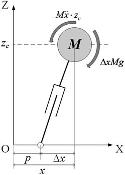
Figure 1 Torque balance for linear inverted pendulum model in the sagittal plane
It is noted that (2) also presents the relationship between ZMP and CoM, and the CoM trajectory can be derived by assigning a suitable ZMP trajectory to (2). For simplicity, the following only presents the derivation of the CoM trajectory in the sagittal plane, namely x(t), and the CoM trajectory in the lateral plane y(t) can be obtained in the same way. Applying Laplace transformation to the first row of (2), we can obtain
 $$\eqalignno{ & {\rm }s^{2} X(s){\minus}sx_{0} {\,\minus\,}v_{{x0}} {\,\equals\,}\omega _{n}^{2} X(s){\,\minus\,}\omega _{n}^{2} P(s) \cr & X(s){\equals}{s \over {{\rm }s^{2} {\minus}\omega _{n}^{2} }}x_{0} {\plus}{1 \over {{\rm }s^{2} {\minus}\omega _{n}^{2} }}v_{{x0}} {\minus}{{\omega _{n}^{2} } \over {{\rm }s^{2} {\minus}\omega _{n}^{2} }}P(s) $$
where x 0 and v x0 denote the initial position and initial velocity of the CoM in the sagittal plane, respectively. P(s) denotes the Laplace transform of the sagittal ZMP trajectory p(t). Then, applying inverse Laplace transformation, the sagittal CoM trajectory x(t) can be obtained as
 $$x(t){\,\equals\,}x_{0} {\rm cosh}(\omega _{n} t){\plus}{{v_{{x0}} } \over {\omega _{n} }}{\rm sinh}(\omega _{n} t){\plus} {\cal L}^{{{\minus}1}} \left( {{{{\minus}\omega _{n}^{2} } \over {{\rm }s^{2} {\minus}\omega _{n}^{2} }}P(s)} \right)$$
where
 $${\cal L}^{{{\minus}1}} ( \cdot )$$
denotes inverse Laplace transform.
$${\cal L}^{{{\minus}1}} ( \cdot )$$
denotes inverse Laplace transform.
Furthermore, the sagittal CoM velocity v x (t) can be obtained as the first derivative of (4):
 $$v_{x} (t){\,\equals\,}x_{0} \omega _{n} {\rm sinh}(\omega _{n} t){\plus}v_{{x0}} {\rm cosh}(\omega _{n} t){\plus}{d \over {dt}}{\cal L}^{{{\minus}1}} \left( {{{{\minus}\omega _{n}^{2} } \over {{\rm }s^{2} {\minus}\omega _{n}^{2} }}P(s)} \right)$$
Since the lateral CoM trajectory y(t) and the lateral CoM velocity v y (t) can be obtained in the same way, the dynamics of CoM in the sagittal and lateral planes can be expressed as follows:
 $$\left[ \matrix{ x(t) \hfill \cr v_{x} (t) \hfill \cr} \right]{\equals}\left[ {\matrix{ {C(t)} & {{1 \over {\omega _{n} }}S(t)} \cr {\omega _{n} S(t)} & {C(t)} \cr } } \right]\left[ \matrix{ x_{0} \hfill \cr v_{{x0}} \hfill \cr} \right]{\plus}\left[ {\matrix{ {\bar{p}(t)} \cr {{d \over {dt}}\bar{p}(t)} \cr } } \right]$$
 $$\left[ \matrix{ y(t) \hfill \cr v_{y} (t) \hfill \cr} \right]{\equals}\left[ {\matrix{ {C(t)} & {{1 \over {\omega _{n} }}S(t)} \cr {\omega _{n} S(t)} & {C(t)} \cr } } \right]\left[ \matrix{ y_{0} \hfill \cr v_{{y0}} \hfill \cr} \right]{\plus}\left[ {\matrix{ {\bar{q}(t)} \cr {{d \over {dt}}\bar{q}(t)} \cr } } \right]$$
with
 $$\bar{p}(t){\,\equals\,}{\cal L}^{{{\minus}1}} \left( {{{{\minus}\omega _{n}^{2} } \over {{\rm }s^{2} {\minus}\omega _{n}^{2} }}P(s)} \right){\rm and}\,\,{\rm }\bar{q}(t){\,\equals\,}{\cal L}^{{{\minus}1}} \left( {{{{\minus}\omega _{n}^{2} } \over {{\rm }s^{2} {\minus}\omega _{n}^{2} }}Q(s)} \right)$$
where y 0 and v y0 denote the initial position and initial velocity of the CoM in the lateral plane, respectively. C(t) and S(t) are defined as cosh(ω n t) and sinh(ω n t), respectively. Q(s) denotes Laplace transform of the lateral ZMP trajectory q(t). It can be seen in (6) and (7) that the first term of the right-hand side is due to the initial conditions, and the second term is due to the given ZMP references.
2.2 Different types of ZMP
To generate a different type of motion it is necessary to utilize different types
of ZMP references. In this paper, five types of ZMP components are considered,
which are step function type, ramp function type, parabolic function type, cubic
function type, and sine function type. In order to use these different types of
ZMP components, it is necessary to know the corresponding
 $$\bar{p}(t)$$
and
$$\bar{p}(t)$$
and
 $$\bar{q}(t)$$
of these components.
$$\bar{q}(t)$$
of these components.
2.2.1 Step function type ZMP
Considering a step function type ZMP p step (t,A s ,T s )=A s u(t−T s), where u(·) is the unit step function, its Laplace transform is
 $$P_{{{\rm step}}} (s){\equals}{{A_{s} } \over s}e^{{{\minus}sT_{s} }} $$
Multiplying by
 $${\minus}\omega _{n}^{2} \,/\,(s^{2} {\minus}\omega _{n}^{2} )$$
and applying inverse Laplace transformation, the second
term of its corresponding CoM trajectory
$${\minus}\omega _{n}^{2} \,/\,(s^{2} {\minus}\omega _{n}^{2} )$$
and applying inverse Laplace transformation, the second
term of its corresponding CoM trajectory
 $$\bar{p}_{{{\rm step}}} $$
can be obtained as follows:
$$\bar{p}_{{{\rm step}}} $$
can be obtained as follows:
 $$\eqalignno{\bar{p}_{{{\rm step}}} (t,A_{s} ,T_{s} ) & {\,\equals\,}{\cal L}^{{{\minus}1}} \left( {{{{\minus}\omega _{n}^{2} } \over {{\rm }s^{2} {\minus}\omega _{n}^{2} }} \cdot {{A_{s} } \over s}e^{{{\minus}sT_{s} }} } \right){\,\equals\,}{\cal L}^{{{\minus}1}} \left( {A_{s} \left[ {{1 \over s}{\minus}{s \over {s^{2} {\minus}\omega _{n}^{2} }}} \right]e^{{{\minus}sT_{s} }} } \right) \cr {\,\equals\,}A_{s} \left[ {1{\minus}{\rm cosh}(\omega _{n} (t{\minus}T_{s} ))} \right]u(t{\minus}T_{s} ) $$
2.2.2 Ramp function type ZMP
Considering a ramp function type ZMP p ramp(t,A r ,T r )=A r tu(t−T r ), its Laplace transform is
 $$P_{{{\rm ramp}}} (s){\equals}{{A_{r} } \over {s^{2} }}(sT_{r} {\plus}1)e^{{{\minus}sT_{r} }} $$
Similarly, the second term of its corresponding CoM trajectory
 $$\bar{p}_{{{\rm ramp}}} $$
can be obtained as follows:
$$\bar{p}_{{{\rm ramp}}} $$
can be obtained as follows:
 $$\bar{p}_{{{\rm ramp}}} (t,A_{r} ,T_{r} ){\equals}A_{r} \left[ {t{\minus}T_{r} {\rm cosh}(\omega _{n} (t{\minus}T_{r} )){\minus}{1 \over {\omega _{n} }}{\rm sinh}(\omega _{n} (t{\minus}T_{r} ))} \right]u(t{\minus}T_{r} )$$
2.2.3 Parabolic function type ZMP
Considering a parabolic function type ZMP p para(t,A p ,T p )=A p t 2 u(t−T p ), its Laplace transform is
 $$P_{{{\rm para}}} (s){\,\equals\,}A_{p} \left( {{{T_{p}^{2} } \over s}{\plus}{{2T_{p} } \over {s^{2} }}{\plus}{2 \over {s^{3} }}} \right)e^{{{\minus}sT_{p} }} $$
Similarly, the second term of its corresponding CoM trajectory
 $$\bar{p}_{{{\rm para}}} $$
can be obtained as follows:
$$\bar{p}_{{{\rm para}}} $$
can be obtained as follows:
 $$\bar{p}_{{{\rm para}}} (t,A_{p} ,T_{p} ){\,\equals\,}A_{p} \left[ {t^{2} {\plus}{2 \over {\omega _{n}^{2} }}{\minus}\left( {T_{p}^{2} {\plus}{2 \over {\omega _{n}^{2} }}} \right){\rm cosh}(\omega _{n} (t{\minus}T_{p} )){\minus}{{2T_{p} } \over {\omega _{n} }}{\rm sinh}(\omega _{n} (t{\minus}T_{p} ))} \right]u(t{\minus}T_{p} )$$
2.2.4 Cubic function type ZMP
Considering a cubic function type ZMP p cubic(t,A c ,T c )=A c t 3 u(t−T c ), its Laplace transform is
 $$P_{{{\rm cubic}}} (s){\,\equals\,}A_{c} \left( {{{T_{c}^{3} } \over s}{\plus}{{3T_{c}^{2} } \over {s^{2} }}{\plus}{{6T_{c} } \over {s^{3} }}{\plus}{6 \over {s^{4} }}} \right)e^{{{\minus}sT_{c} }} $$
Similarly, the second term of its corresponding CoM trajectory
 $$\bar{p}_{{{\rm cubic}}} $$
can be obtained as follows:
$$\bar{p}_{{{\rm cubic}}} $$
can be obtained as follows:
 $$\eqalignno{\bar{p}_{{{\rm cubic}}} (t,A_{c} ,T_{c} ) {\,\equals\,} &A_{c} \left[ {t^{3} {\plus}{6 \over {\omega _{n}^{2} }}t{\plus}2T_{c}^{3} {\minus}\left( {T_{c}^{3} {\plus}{{6T_{c} } \over {\omega _{n}^{2} }}} \right){\rm cosh}(\omega _{n} (t{\minus}T_{c} ))} \right. \cr \left. {{\rm }{\minus}\left( {{{3T_{c}^{2} } \over {\omega _{n} }}{\plus}{6 \over {\omega _{n}^{3} }}} \right){\rm sinh}(\omega _{n} (t{\minus}T_{c} ))} \right]u(t{\minus}T_{c} ){\rm } $$
2.2.5 Sine function type ZMP
Considering a sine function type ZMP
 $$p_{{{\rm sin}}} (t,A_{\beta } ,\alpha ,T_{\beta } ){\,\equals\,}A_{\beta } {\rm sin}(\alpha t)u(t{\minus}T_{\beta } )$$
, its Laplace transform is
$$p_{{{\rm sin}}} (t,A_{\beta } ,\alpha ,T_{\beta } ){\,\equals\,}A_{\beta } {\rm sin}(\alpha t)u(t{\minus}T_{\beta } )$$
, its Laplace transform is
 $$P_{{{\rm sin}}} (s){\equals}(\phi _{s} s{\plus}\psi _{s} ){{e^{{{\minus}sT_{\beta } }} } \over {s^{2} {\plus}\alpha ^{2} }}$$
where ϕ s =A β sin(αT β ) and ψ s =αA β cos(αT β ).
Similarly, the second term of its corresponding CoM trajectory
 $$\bar{p}_{{{\rm sin}}} $$
can be obtained as follows:
$$\bar{p}_{{{\rm sin}}} $$
can be obtained as follows:
 $$\eqalignno{\bar{p}_{{{\rm sin}}} (t,A_{\beta } ,\alpha ,T_{\beta } ){\,\equals\,} & {1 \over {\alpha ^{2} {\plus}\omega _{n}^{2} }}\left[ {\phi _{s} \omega _{n}^{2} {\rm cos}(\alpha (t{\minus}T_{\beta } )){\plus}{{\psi _{s} } \over \alpha }\omega _{n}^{2} {\rm sin}(\alpha (t{\minus}T_{\beta } ))} \right. \cr {\rm }\left. {{\minus}\phi _{s} \omega _{n}^{2} {\rm cosh}(\omega _{n} (t{\minus}T_{\beta } )){\minus}\psi _{s} \omega _{n} {\rm sinh}(\omega _{n} (t{\minus}T_{\beta } ))} \right]u(t{\minus}T_{\beta } ) $$
In addition, for a cosine function type ZMP p
cos(t,A
β
,a,T
β
)=A
β
cos(αt)u(t−T
β
), the second term of its corresponding CoM trajectory
 $$\bar{p}_{{{\rm cos}}} $$
is
$$\bar{p}_{{{\rm cos}}} $$
is
 $$\eqalignno{\bar{p}_{{{\rm cos}}} (t,A_{\beta } ,\alpha ,T_{\beta } ){\,\equals\,}&{1 \over {\alpha ^{2} {\plus}\omega _{n}^{2} }}\left[ {\phi _{c} \omega _{n}^{2} {\rm cos}(\alpha (t{\minus}T_{\beta } )){\plus}{{\psi _{c} } \over \alpha }\omega _{n}^{2} {\rm sin}(\alpha (t{\minus}T_{\beta } ))} \right. \cr {\rm }\left. {{\minus}\phi _{c} \omega _{n}^{2} {\rm cosh}(\omega _{n} (t{\minus}T_{\beta } )){\minus}\psi _{c} \omega _{n} {\rm sinh}(\omega _{n} (t{\minus}T_{\beta } ))} \right]u(t{\minus}T_{\beta } ) $$
where ϕ c =A β cos αT β and ψ c =−αA β sin αT β .
2.3 Center of mass trajectory generation by given ZMP references
So far, by being given a suitable ZMP reference and suitable initial conditions, the CoM trajectory can be acquired with (6) and (7). However, there is a problem when using (6) and (7) to calculate the CoM trajectory since there are cosh term and sinh term in (6) and (7). The value of cosh term and sinh term tend to infinity as t becomes much greater than 0. Hence, a complete gait pattern is divided into several partitions according to the number of steps, and the CoM trajectory is generated step by step with given boundary conditions for each step. Hereafter, the CoM trajectory will be discussed for a single step.
2.3.1 Common ZMP reference
Generally, the most common ZMP reference for a single step is defined as follows:
 $$\left\{ \matrix{ p_{n} (t){\,\equals\,}A_{n} u(t) \hfill \cr q_{n} (t){\,\equals\,}B_{n} u(t) \hfill \cr} \right.\,{\rm }{\rm for}\,t\in(0,T]$$
where T denotes the period of a step, which is half of the walking period. Subscript n denotes the nth step. A n and B n denote sagittal amplitude and lateral amplitude of ZMP for the nth step. Since the following discusses the CoM trajectory of a single step as well, the subscript n will be omitted for simplicity when there is no ambiguity.
2.3.2 Double support phase ZMP reference
It is obvious that the common ZMP reference does not consider DSP. On the other hand, a ZMP reference taking into account DSP can be expressed as follows:
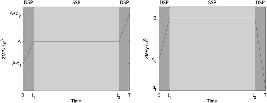
 $$\left\{ \matrix{ p^{{\rm D}} (t){\,\equals\,}\left( {A{\minus}d_{1} {\plus}{{d_{1} } \over {k_{v} T}}t} \right)\left[ {u(t){\minus}u(t{\minus}t_{1} )} \right]{\plus}A\left[ {u(t{\minus}t_{1} ){\minus}u(t{\minus}t_{2} )} \right]{\plus}\left[ {A{\plus}{{d_{2} } \over {k_{v} T}}(t{\minus}t_{2} )} \right]u(t{\minus}t_{2} ) \hfill \cr q^{{\rm D}} (t){\,\equals\,}\left( {q_{0} {\plus}{{B{\minus}q_{0} } \over {k_{v} T}}t} \right)\left[ {u(t){\minus}u(t{\minus}t_{1} )} \right]{\plus}B\left[ {u(t{\minus}t_{1} ){\minus}u(t{\minus}t_{2} )} \right]{\plus}\left[ {B{\plus}{{q_{f} {\minus}B} \over {k_{v} T}}(t{\minus}t_{2} )} \right]u(t{\minus}t_{2} ) \hfill \cr} \right.$$
where A−d 1 and A+d 2 are initial and final positions of p, respectively, and q 0 and q f are initial and final positions of q, respectively. It is noted that when walking in a straight line, the values of q 0 and q f are usually set as 0, namely q 0=q f =0. A, B and the initial and final positions of p and q are user-defined parameters for designing a desired ZMP reference, and these parameters are determined by a parameterized gait planning algorithm in this paper, which will be examined in Section 3. Superscript D denotes the ZMP reference taking into account DSP, k v denotes virtual DSP scale, t 1 is k v T, and t 2 is (1−k v T). As shown in Figure 2, the DSP-ZMP reference is composed of three intervals. The first interval is a DSP whose range is (0, t 1]. The second phase is an SSP whose range is (t 1, t 2]. The third interval is a DSP whose range is (t 2, T]. ZMP moves within the DSP and stays at a fixed point within the SSP. In addition, d 1 and d 2 denote the incremental amount of sagittal amplitude within the first interval and the third interval, respectively. It is important that d 1 and d 2 should be positive since the gait pattern is generated for walking forward.

Figure 2 DSP-ZMP reference. SSP=single support phase; DSP=double support phase
2.3.3 Moving ZMP reference
In human walking, ZMP moves continuously even during SSP. Thus, Erbatur and Kurt (Reference Erbatur and Kurt2009) defined a ZMP reference with ZMP moving forward slightly during SSP as a natural ZMP reference. Inspired by this concept, we define a moving ZMP reference as follows:
 $$\left\{ \matrix{ p^{{\rm M}} (t){\equals}\left( {A{\minus}d_{1} {\plus}{{d_{1} {\minus}a} \over {k_{v} T}}t} \right)\left[ {u(t){\minus}u(t{\minus}t_{1} )} \right]{\plus}\left[ {A{\minus}a{\plus}{{2a} \over {(1{\minus}2k_{v} )T}}(t{\minus}t_{1} )} \right]\left[ {u(t{\minus}t_{1} ){\minus}u(t{\minus}t_{2} )} \right]\cr \qquad\quad{\plus} \left[ {A{\plus}a{\plus}{{d_{2} {\minus}a} \over {k_{v} T}}(t{\minus}t_{2} )} \right]u(t{\minus}t_{2} ) \hfill \cr q^{{\rm M}} (t){\equals}\left( {q_{0} {\plus}{{B{\minus}q_{0} } \over {k_{v} T}}t} \right)\left[ {u(t){\minus}u(t{\minus}t_{1} )} \right]{\plus}\left[ {B{\plus}b{\rm sin}\left( {{\pi \over {(1{\minus}2k_{v} )T}}(t{\minus}t_{1} )} \right)} \right]\left[ {u(t{\minus}t_{1} ){\minus}u(t{\minus}t_{2} )} \right]\cr \qquad\quad{\plus} \left[ {B{\plus}{{q_{f} {\minus}B} \over {k_{v} T}}(t{\minus}t_{2} )} \right]u(t{\minus}t_{2} ) \hfill \cr} \right.$$
where a denotes half of the distance that ZMP moves forward during an SSP, and b denotes the incremental amount of lateral amplitude during an SSP. It is noted that B and b must have the same sign. In addition, the DSP-ZMP reference is a special case of a moving ZMP reference while a=0 and b=0.
With the proposed moving ZMP reference, the ZMP can move during SSP not only in the sagittal plane but also in the lateral plane, which makes the robot walk more naturally and in a more human-like way. To obtain the corresponding CoM trajectory of the moving ZMP reference, (21) can be rewritten as follows:
 $$\left\{ \matrix{ p^{{\rm M}} (t){\equals}(L_{{p1}} {\plus}K_{{p1}} t)\left[ {u(t){\minus}u(t{\minus}t_{1} )} \right]{\plus}(L_{{p2}} {\plus}K_{{p2}} t)\left[ {u(t{\minus}t_{1} ){\minus}u(t{\minus}t_{2} )} \right] \hfill \cr \!\!\quad\qquad \,\,{\plus} (L_{{p3}} {\plus}K_{{p3}} t)u(t{\minus}t_{2} ) \hfill \cr q^{{\rm M}} (t){\equals}(L_{{q1}} {\plus}K_{{q1}} t)\left[ {u(t){\minus}u(t{\minus}t_{1} )} \right]{\plus}\left[ {L_{{q2}} {\plus}K_{{q2}} {\rm sin}(\alpha t{\minus}t_{d} )} \right]\left[ {u(t{\minus}t_{1} ){\minus}u(t{\minus}t_{2} )} \right] \cr \!\!\quad\qquad \,\,{\plus} (L_{{q3}} {\plus}K_{{q3}} t)u(t{\minus}t_{2} ) \hfill \cr} \right.$$
with
 $$\eqalignno{ & L_{{p1}} {\,\equals\,}A{\minus}d_{1} ,\,L_{{p2}} {\,\equals\,}A{\minus}a{\minus}{{2at_{1} } \over {(1{\minus}2k_{v} )T}},\,L_{{p3}} {\,\equals\,}A{\plus}a{\minus}{{(d_{2} {\minus}a)t_{2} } \over {k_{v} T}} \cr & K_{{p1}} {\,\equals\,}{{d_{1} {\minus}a} \over {k_{v} T}},\,K_{{p2}} {\,\equals\,}{{2a} \over {(1{\minus}2k_{v} )T}},\,K_{{p3}} {\,\equals\,}{{d_{2} {\minus}a} \over {k_{v} T}} \cr & L_{{q1}} {\,\equals\,}q_{0} ,\,L_{{q2}} {\,\equals\,}B,\,L_{{q3}} {\,\equals\,}B{\minus}{{(q_{f} {\minus}B)t_{2} } \over {k_{v} T}} \cr & K_{{q1}} {\equals}{{B{\minus}q_{0} } \over {k_{v} T}},\,K_{{q2}} {\,\equals\,}b,\,K_{{q3}} {\,\equals\,}{{q_{f} {\minus}B} \over {k_{v} T}},\,\alpha {\,\equals\,}{\pi \over {(1{\minus}2k_{v} )T}}{\rm ,}\,t_{d} {\,\equals\,}\alpha t_{1} $$
Since p
M(t) and q
M(t) are linear combinations of step, ramp, and
sine function type ZMP,
 $$\bar{p}^{{\rm M}} (t)$$
and
$$\bar{p}^{{\rm M}} (t)$$
and
 $$\bar{q}^{{\rm M}} (t)$$
of the moving ZMP reference can be obtained using (9),
(11), (17), and (18) as follows:
$$\bar{q}^{{\rm M}} (t)$$
of the moving ZMP reference can be obtained using (9),
(11), (17), and (18) as follows:
 $$\eqalignno{\bar{p}^{{\rm M}} (t){\,\equals\,}&\bar{p}_{{{\rm step}}} (t,L_{{p1}} ,0){\plus}\bar{p}_{{{\rm ramp}}} (t,K_{{p1}} ,0){\plus}\bar{p}_{{{\rm step}}} (t,L_{{p2}} {\minus}L_{{p1}} ,t_{1} ){\plus}\bar{p}_{{{\rm ramp}}} (t,K_{{p2}} {\minus}K_{{p1}} ,t_{1} ) \cr\!\!{\plus}{\rm }\bar{p}_{{{\rm step}}} (t,L_{{p3}} {\minus}L_{{p2}} ,t_{2} ){\plus}\bar{p}_{{{\rm ramp}}} (t,K_{{p3}} {\minus}K_{{p2}} ,t_{2} ) $$
 $$\eqalignno{\bar{q}^{{\rm D}} (t){\,\equals\,}&\bar{p}_{{{\rm step}}} (t,L_{{q1}} ,0){\plus}\bar{p}_{{{\rm ramp}}} (t,K_{{q1}} ,0){\plus}\bar{p}_{{{\rm step}}} (t,L_{{q2}} {\minus}L_{{q1}} ,t_{1} ){\plus}\bar{p}_{{{\rm ramp}}} (t,{\minus}K_{{q1}} ,t_{1} ) \cr\!\! {\plus}{\rm cos}(t_{d} )\bar{p}_{{{\rm sin}}} (t,K_{{q2}} ,\alpha ,t_{1} ){\minus}{\rm sin}(t_{d} )\bar{p}_{{{\rm cos}}} (t,K_{{q2}} ,\alpha ,t_{1} ) \cr\!\! {\plus}{\rm }\bar{p}_{{{\rm step}}} (t,L_{{q3}} {\minus}L_{{q2}} ,t_{2} ){\plus}\bar{p}_{{{\rm ramp}}} (t,K_{{q3}} ,t_{2} ){\minus}{\rm cos}(t_{d} )\bar{p}_{{{\rm sin}}} (t,K_{{q2}} ,\alpha ,t_{2} ){\plus}{\rm sin}(t_{d} )\bar{p}_{{{\rm cos}}} (t,K_{{q2}} ,\alpha ,t_{2} ) $$
So far, the corresponding CoM trajectory of the moving reference can be
obtained by substituting (23) and (24) into (6) and (7), respectively.
However, the initial conditions of the DSP-ZMP reference are still unknown.
To determine the initial conditions, we define the boundary conditions of
the CoM trajectory as initial and final positions of ZMP, namely
 $$x_{0}^{{\rm M}} {\,\equals\,}p^{{\rm M}} (0){\,\equals\,}A{\minus}d_{1} $$
, x
M(T)=p
M(T)=A+d
2,
$$x_{0}^{{\rm M}} {\,\equals\,}p^{{\rm M}} (0){\,\equals\,}A{\minus}d_{1} $$
, x
M(T)=p
M(T)=A+d
2,
 $$y_{0}^{{\rm M}} {\,\equals\,}q^{{\rm M}} (0){\,\equals\,}q_{0} $$
, and y
M(T)=q
M(T)=q
f
. Then, substituting these boundary conditions into the first row of
(6) and (7), the initial velocity of a moving reference can be obtained
as
$$y_{0}^{{\rm M}} {\,\equals\,}q^{{\rm M}} (0){\,\equals\,}q_{0} $$
, and y
M(T)=q
M(T)=q
f
. Then, substituting these boundary conditions into the first row of
(6) and (7), the initial velocity of a moving reference can be obtained
as
 $$\left\{ \matrix{ v_{{x0}}^{{\rm M}} {\equals}{{\omega _{n} } \over {S(T)}}\left[ {x^{{\rm M}} (T){\minus}C(T)x_{0}^{{\rm M}} {\minus}\bar{p}^{{\rm M}} (T)} \right]{\equals}{{\omega _{n} } \over {S(T)}}\left[ {A{\plus}d_{2} {\minus}C(T)(A{\minus}d_{1} ){\minus}\bar{p}^{{\rm M}} (T)} \right] \hfill \cr v_{{y0}}^{{\rm M}} {\equals}{{\omega _{n} } \over {S(T)}}\left[ {y^{{\rm M}} (T){\minus}C(T)y_{0}^{{\rm M}} {\minus}\bar{q}^{{\rm M}} (T)} \right]{\equals}{{\omega _{n} } \over {S(T)}}\left[ {q_{f} {\minus}C(T)q_{{\rm 0}} {\minus}\bar{q}^{{\rm M}} (T)} \right] \hfill \cr} \right.$$
Figure 3 shows a moving ZMP reference with two steps. A 1 and A 2 are 0.1 and 0.15, respectively. B 1 and B 2 are 0.075 and −0.075, respectively. d 1 and d 2 of both steps are set as 0.025, and q 0 and q f of both steps are set as 0. a of both steps are set as 0.01. b 1 and b 2 are set as 0.01 and −0.01, respectively. T and z c are set as 1 second and 0.52975 m, respectively. Figure 3(a, b) shows CoM trajectories of the moving ZMP reference without DSP. Figure 3(c, d) shows CoM trajectories of the moving ZMP reference with DSP, and k v is set as 0.1. It can be seen that at the boundary (T=1 second), the velocity of the moving ZMP reference with DSP is smoother than that of the moving ZMP reference without DSP. Velocity smoothness means the velocity is continuous derivative at boundaries. Hence, the ZMP reference with DSP is more reliable because of its smooth transition.
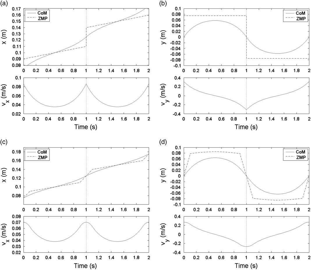
Figure 3 Corresponding center of mass (CoM) trajectories of moving ZMP references without double support phase (DSP) and with DSP. In the top of (a) and (c), the solid line and the dashed line denote the CoM trajectory and ZMP trajectory in x-axis, respectively. In the bottom of (a) and (c), vx denotes velocity of CoM in x-axis. Similarly, in the top of (b) and (d), the solid line and the dashed line denote the CoM trajectory and ZMP trajectory in y-axis, respectively. In the bottom of (b) and (d), vy denotes velocity of CoM in y-axis.
3 Parameterized gait planning algorithm
In Section 2.3, a CoM trajectory with the moving ZMP reference has been introduced. In order to generate a complete gait pattern using the proposed CoM trajectory with desired footprint location, a parameterized gait planning algorithm is presented in this section. Once the user-defined parameters are determined, the initial conditions and CoM trajectory for each step can be obtained and the overall gait pattern can be acquired using the gait planning algorithm. The gait planning algorithm consists of the following steps:
-
i. Determine the user-defined parameters including step period T, step height H, step width W, number of steps N, virtual DSP ratio k v , and DSP ratio k. It is noted that the period of DSP is defined by k instead of k v . The period of DSP T DSP is 2kT and the period of SSP T SSP is (1−2k)T. The range of k is set as (0, 0.25] so that T DSP will not be greater than half of the period T and there is sufficient time for the swing leg to step forward. k v is used to tune the boundary velocities for a smooth transition between steps.
-
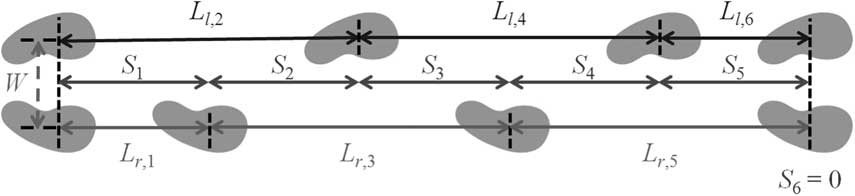
ii. Determine the step size of each step S n for n∈{1, 2, … , N}, and it is important that S N should be 0 so that the walking distances of both legs can be identical. Then, as in the footprint definition shown in Figure 4, stride length L n can be obtained as L n =S n +S n−1 for n∈{1, 2, … , N} with S 0=0.
Furthermore, assuming the first swing leg is the right leg of the robot, the stride length of a specific leg for each step is defined as follows:
(26) $$L_{{r,n}} {\equals}\left\{ \matrix{ L_{n} ,\,{\rm }{\rm for}\,n{\,\equals\,}\left\{ {{\rm 2}i{\minus}1\left| {\forall i\in{\Bbb N}^{{\plus}} ,\,2i{\,\minus\,}1 ⩽ \,N} \right.} \right\} \hfill \cr 0,\,{\rm }{\rm for}\,n{\,\equals\,}\left\{ {{\rm 2}i\left| {\forall i\in{\Bbb N}^{{\plus}} ,\,2i \,⩽ \,N} \right.} \right\} \hfill \cr} \right.$$
(27)
$$L_{{l,n}} {\equals}\left\{ \matrix{ 0,\,{\rm }{\rm for}\,n{\,\equals\,}\left\{ {{\rm 2}i{\minus}1\left| {\forall i\in{\Bbb N}^{{\plus}} ,\,2i{\minus}1\,⩽ \,N} \right.} \right\} \hfill \cr L_{n} ,\,{\rm }{\rm for}\,n{\,\equals\,}\left\{ {{\rm 2}i\left| {\forall i\in{\Bbb N}^{{\plus}} ,\,2i\,⩽ \,N} \right.} \right\} \hfill \cr} \right.$$
$$L_{{r,n}} {\equals}\left\{ \matrix{ L_{n} ,\,{\rm }{\rm for}\,n{\,\equals\,}\left\{ {{\rm 2}i{\minus}1\left| {\forall i\in{\Bbb N}^{{\plus}} ,\,2i{\,\minus\,}1 ⩽ \,N} \right.} \right\} \hfill \cr 0,\,{\rm }{\rm for}\,n{\,\equals\,}\left\{ {{\rm 2}i\left| {\forall i\in{\Bbb N}^{{\plus}} ,\,2i \,⩽ \,N} \right.} \right\} \hfill \cr} \right.$$
(27)
$$L_{{l,n}} {\equals}\left\{ \matrix{ 0,\,{\rm }{\rm for}\,n{\,\equals\,}\left\{ {{\rm 2}i{\minus}1\left| {\forall i\in{\Bbb N}^{{\plus}} ,\,2i{\minus}1\,⩽ \,N} \right.} \right\} \hfill \cr L_{n} ,\,{\rm }{\rm for}\,n{\,\equals\,}\left\{ {{\rm 2}i\left| {\forall i\in{\Bbb N}^{{\plus}} ,\,2i\,⩽ \,N} \right.} \right\} \hfill \cr} \right.$$
where L r,n and L l,n denote the stride length of the right and left legs for the nth step, respectively. For example, if the robot takes four steps and S=[0.05, 0.05, 0.05, 0], then L r =[0.05, 0, 0.1, 0] and L l =[0, 0.1, 0, 0.05].
-
iii. Calculate the sagittal amplitude of each step, namely A n for n∈{1, 2, … , N}. A n is defined as
(28)
$$A_{n} {\,\equals\,}L_{{n{\minus}1}} {\plus}A_{{n{\minus}2}} \,{\rm for}\,n\in\{ 2,\,\ldots\,,\,N\} $$
with A 0=0 and A 1=0. It is noted that A 0 is just a virtual sagittal amplitude for calculating A n and is not used in the following steps. A 1 is defined as 0 so that the robot can walk with zero initial velocity.
-
iv. Determine B n , a n , and b n for each step. Generally, if step width W is identical for all steps, then B n can be defined as
(29)
$$B_{n} {\,\equals\,}{{({\minus}1)^{{n{\minus}1}} W} \mathord{\left/ {\vphantom {{({\minus}1)^{{n{\minus}1}} W} 2}} \right. \kern-\nulldelimiterspace} 2}\,{\rm for}\,n\in\{ 1,\,\ldots\,,\,N\} $$
a n and b n should be relatively small values to A n and B n , respectively.
-
v. Calculate the boundary conditions for each step, namely A n −d 1,n , A n +d 2,n , q 0,n , and q f,n for n∈{1, 2, … , N}. In order to accelerate from zero initial velocity at the first step and decelerate to zero final velocity at the final step in the sagittal plane, d 1,1 and d 2,N are set as 0. d 2 of the other steps are defined as follows:
(30)
$$d_{{2,n}} {\equals}{{A_{{n{\plus}1}} {\minus}A_{n} } \over 2}\,{\rm for}\,n\in{\rm \{ 1, }...{\rm ,}\,N{\minus}1{\rm \} }$$
In addition, since the initial position of a step must be the same as the final position of its previous step, we can know
(31)
$$d_{{1,n{\plus}1}} {\,\equals\,}d_{{2,n}} \,{\rm for}\,n\in{\rm \{ 1, }...{\rm ,}\,N{\minus}1{\rm \} }$$
Similarly, q 0,1 and q f,N are set as 0, and q 0 and q f of the other step are defined as
(32)
$$q_{{f,n}} {\,\equals\,}{{B_{{n{\plus}1}} {\plus}B_{n} } \over 2}\,{\rm for}\,n\in{\rm \{ 1, }...{\rm ,}\,N{\minus}1{\rm \} }$$
(33)
$$q_{{_{{0,n{\plus}1}} }} {\,\equals\,}q_{{_{{f,n}} }} \,{\rm for}\,n\in{\rm \{ 1,}\,\ldots\,,\,N{\minus}1{\rm \} }$$
-
vi. Calculate the initial position and the initial velocity for each step with (25).
-
vii. Calculate the CoM trajectory step by step with (6) and (7).
-
viii. Concatenate the CoM trajectories of all steps together to obtain the complete CoM trajectory as follows
(34)
$$x(t){\equals}\mathop{\sum}\limits_{n{\equals}1}^N {x_{n} (t{\minus}(n{\minus}1)T)\left[ {u(t{\minus}(n{\minus}1)T){\minus}u(t{\minus}nT)} \right]} $$
(35)
$$y(t){\equals}\mathop{\sum}\limits_{n{\equals}1}^N {y_{n} (t{\minus}(n{\minus}1)T)\left[ {u(t{\minus}(n{\minus}1)T){\minus}u(t{\minus}nT)} \right]} $$
-
ix. Calculate the foot trajectories with respect to the world coordinate system. The foot trajectory generation is divided into two parts. Swing foot trajectory is obtained using a rolling cycle (Liu et al., Reference Liu, Wang and Chen2013), and the supporting foot trajectory stays at a fixed point. Thus, the foot trajectories for nth step are defined as
(36)
$$footx_{{j,n}} (t){\equals}\left\{ \matrix{ 0,\!\!\qquad\quad\qquad{\rm }{\rm if}\,t \,⩽ \, t_{{\rm 1}} \hfill \cr {{L_{{j,n}} } \over {2\pi }}(\theta {\minus}\sin \theta ),{\rm }{\rm if}\,t_{{\rm 1}} \,\lt\,t \, ⩽ \, t_{{\rm 2}} \hfill \cr L_{{j,n}} {\rm , }\qquad\qquad{\rm otherwise} \hfill \cr} \right.$$
(37)
$$footy_{{l,n}} (t){\equals}{1 \over 2}W\,{\rm and}\,\,{\rm }footy_{{r,n}} (t){\equals}{\minus}{1 \over 2}W$$
(38)
$$footz_{{j,n}} (t){\equals}\left\{ \matrix{ {H \over 2}(1{\minus}{\rm cos}\,\theta ),{\rm }{\rm if}\,t_{{\rm 1}} \,\lt\,t \, ⩽ \, t_{{\rm 2}} \hfill \cr 0,\qquad\qquad{\rm otherwise} \hfill \cr} \right.$$
where t 1=kT, t 2 =(1−k)T, θ=2π(t−t 1)/(t 2−t 1), and t∈(0,T]. j∈{r, l}, r and l denote the right foot and the left foot, respectively.
Then, a complete foot trajectory with respect to the world coordinate system can be obtained as follows:
(39)
$$footx_{j} (t){\equals}\mathop{\sum}\limits_{n{\equals}1}^N {\left[ {O_{{j,n}} {\plus}footx_{{j,n}} (t{\minus}(n{\minus}1)T)} \right]\left[ {u(t{\minus}(n{\minus}1)T){\minus}u(t{\minus}nT)} \right]} $$
(40)
$$footy_{l} (t){\equals}{1 \over 2}W\,{\rm and}\,\,{\rm }footy_{r} (t){\equals}{\minus}{1 \over 2}W$$
(41)
$$footz_{j} {\equals}\mathop{\sum}\limits_{n{\equals}1}^N {footz_{{j,n}} (t{\minus}(n{\minus}1)T)\left[ {u(t{\minus}(n{\minus}1)T){\minus}u(t{\minus}nT)} \right]} $$
with O j,1=0,
$$O_{{j,n}} {\equals}\mathop{\sum}\limits_{m{\equals}1}^{n{\minus}1} {L_{{j,m}} } \,{\rm for}\,n\in\{ 2,\,\ldots\,,\,N\} $$
and j∈{r,
l}. -
x. Finally, calculate the foot trajectories with respect to the joint coordinate system and apply inverse kinematics.


Figure 4 Definitions of step size and stride length for footprint location
4 Experiments
Parameterized gait patterns have been generated for the teen-sized humanoid robot, David Junior, which is 96 cm tall and weighs about 9.4 kg. The CoM height z c of David is 52.975 cm. David has 26 d.f. as shown in Figure 5. Each leg consists of 6 d.f. and weighs 2.177 kg. Each arm consists of 5 d.f., and the mass of the upper body with arms is 4.96 kg.
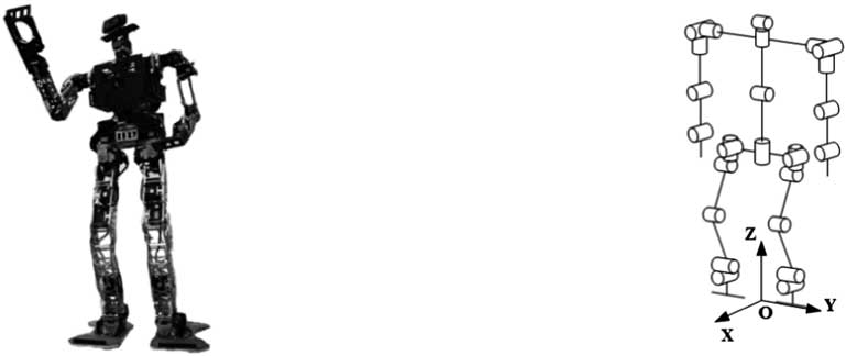
Figure 5 Teen-sized humanoid robot, David Junior
The gait patterns consist of eight steps (four walking cycles), namely N=8. The first swing leg is assigned the right leg. The step period T was set as 0.85 seconds and DSP ratio k was set as 0.22. Thus, DSP period T DSP was 0.374 seconds and SSP period T SSP was 0.476 seconds. The magnitude of the lateral amplitude was set as 8 cm, so B=[8, −8, 8, −8, 8, −8, 8, −8] cm. a n for all steps were set as 0.5 cm. b was set as [0.5, −0.5, 0.5, −0.5, 0.5, −0.5, 0.5, −0.5] cm. Virtual DSP ratio k v was set as 0.1. To demonstrate the feasibility of the proposed method, two different gait patterns were generated with different step size S. Step height H was set as 3 cm.
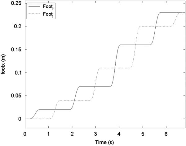
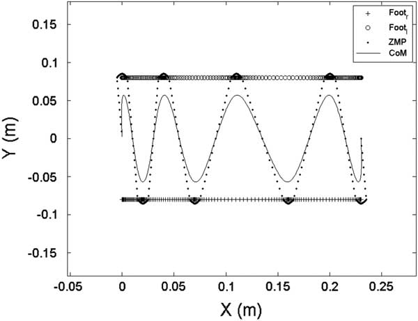
In the first gait pattern, each step size was set as 5 cm except the final step, namely S=[5, 5, 5, 5, 5, 5, 5, 0] cm. Figures 6 and 7 show the sagittal and lateral trajectory of CoM, respectively. Figure 8 shows foot trajectories with respect to X-axis and Z-axis. Figure 9 shows the ZMP reference and the CoM trajectory of the first gait pattern in XY plane. Foot trajectories of both legs depicted with plus sign markers are also shown in Figure 9.
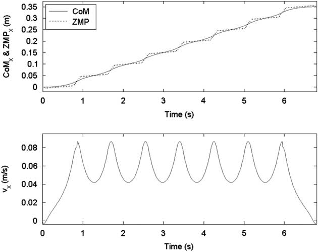
Figure 6 ZMP reference and center of mass (CoM) trajectory in the sagittal plane for the first gait pattern

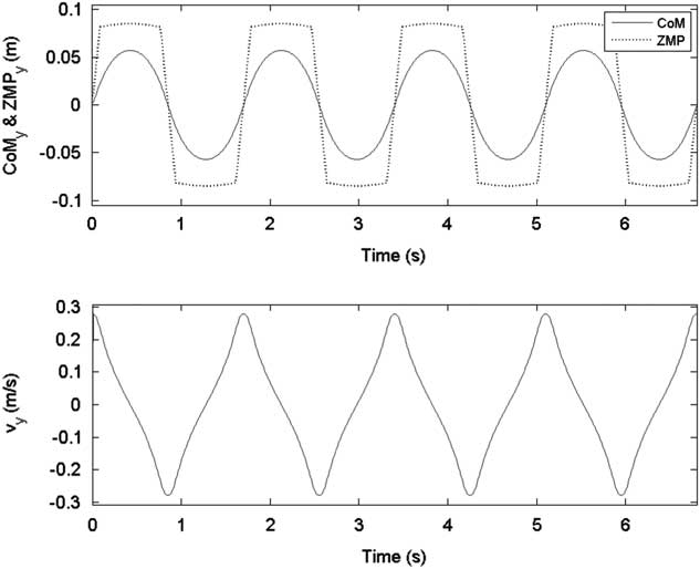
Figure 7 ZMP reference and center of mass (CoM) trajectory in the lateral plane

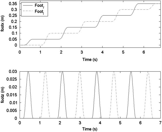
Figure 8 Foot trajectories for the first gait pattern
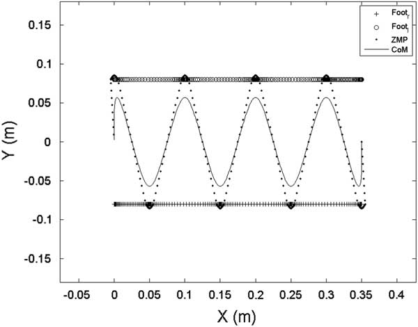
Figure 9 ZMP reference and center of mass (CoM) trajectory in the XY plane for the first gait pattern
In the second gait pattern, S was set as [2, 2, 3, 4, 5, 4, 3, 0] cm. The lateral CoM trajectory of the second gait pattern was set the same as in the first gait pattern, and the sagittal CoM trajectory is shown in Figure 10. Foot trajectories with respect to the X-axis are shown in Figure 11. Figure 12 shows the ZMP reference, CoM trajectory, and foot trajectories of both legs in the XY plane.
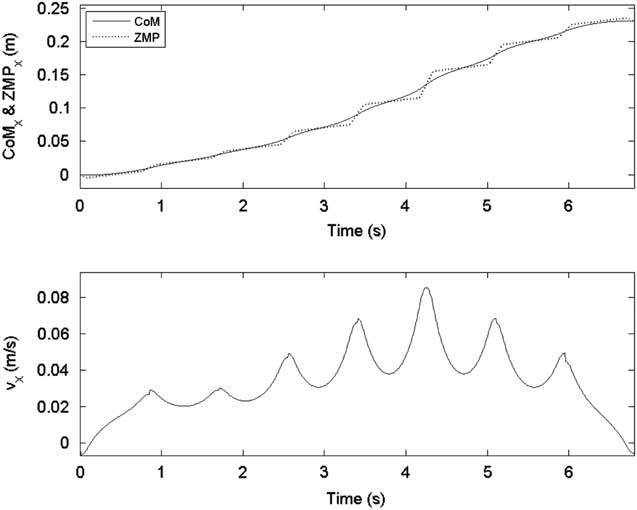
Figure 10 ZMP reference and center of mass (CoM) trajectory in the sagittal plane for the second gait pattern

Figure 11 Foot trajectories with respect to the X-axis for the second gait pattern

Figure 12 ZMP reference and center of mass (CoM) trajectory in the XY plane for the second gait pattern
To verify that the moving ZMP reference with DSP is more reliable than the moving ZMP reference without DSP, a simulation study was carried out on Webots (Michel, Reference Vukobratović and Stepanenko2004), which is a powerful robot simulator widely used in robotic research. Both of the gait patterns mentioned above were performed in the simulator, and actual ZMP trajectories were measured for verification. The robot model of the simulation was modeled based on the specification of David as shown in Figure 13. Although there is modeling error between the real robot and the simulation model, the simulation results are still reliable.
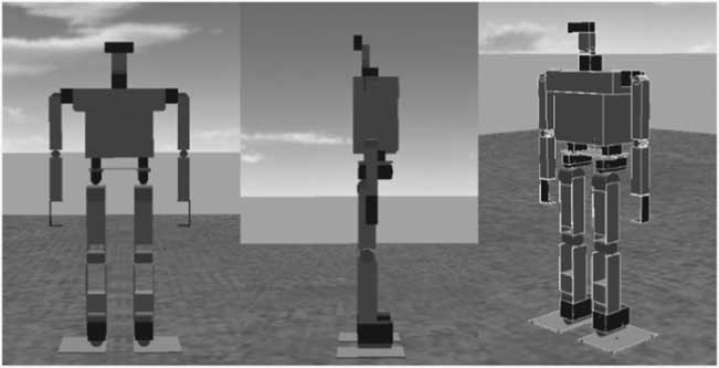
Figure 13 The model of David in the robot simulator
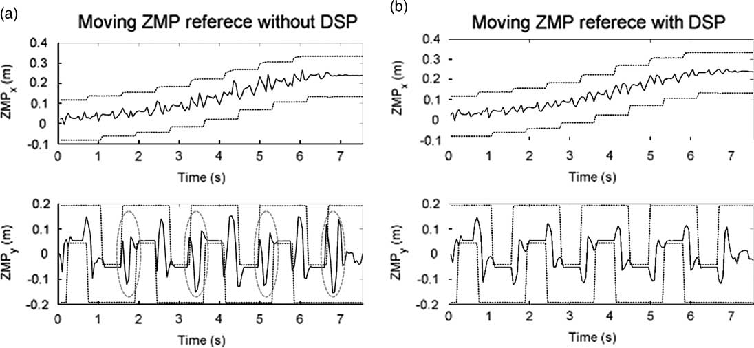
Four force sensors are equipped underneath the corners of each sole to measure actual ZMP trajectories. The measured ZMP trajectories of the first and the second gait pattern are shown in Figures 14 and 15, respectively. The solid lines denote the measured ZMP trajectory and the dotted lines denotes the boundaries of foot trajectory in Figures 14 and 15. It can be seen that the measured ZMP trajectory of the ZMP reference with DSP is more regular than that of the ZMP reference without DSP, and vibration of the former is also smaller. Furthermore, in Figures 14(a) and 15(a), it can be seen that overshoot occurs while support phase transitions. It is especially serious at the transitions marked with the red circles because ZMP almost exceeds the boundary of the support polygon. Therefore, the reliability of the moving ZMP reference with DSP can be verified with this simulation.
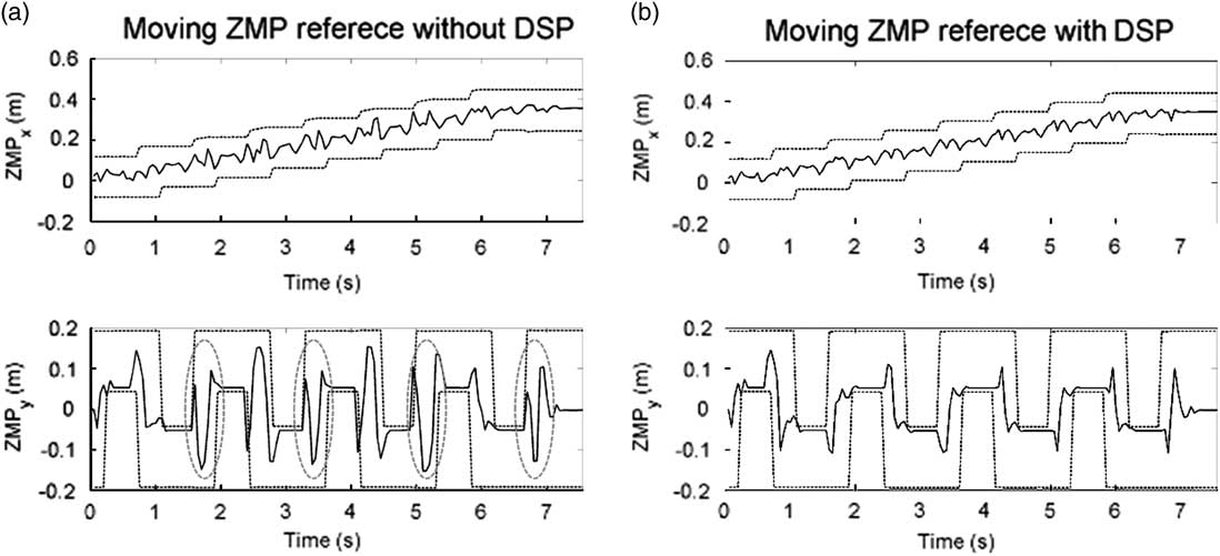
Figure 14 Measured ZMP trajectory of the first gait pattern. DSP=double support phase. ZMPx denotes the x coordinate of the ZMP, and ZMPy denotes the y coordinate of the ZMP

Figure 15 Measured ZMP trajectory of the second gait pattern. ZMPx denotes the x coordinate of the ZMP, and ZMPy denotes the y coordinate of the ZMP. DSP=double support phase
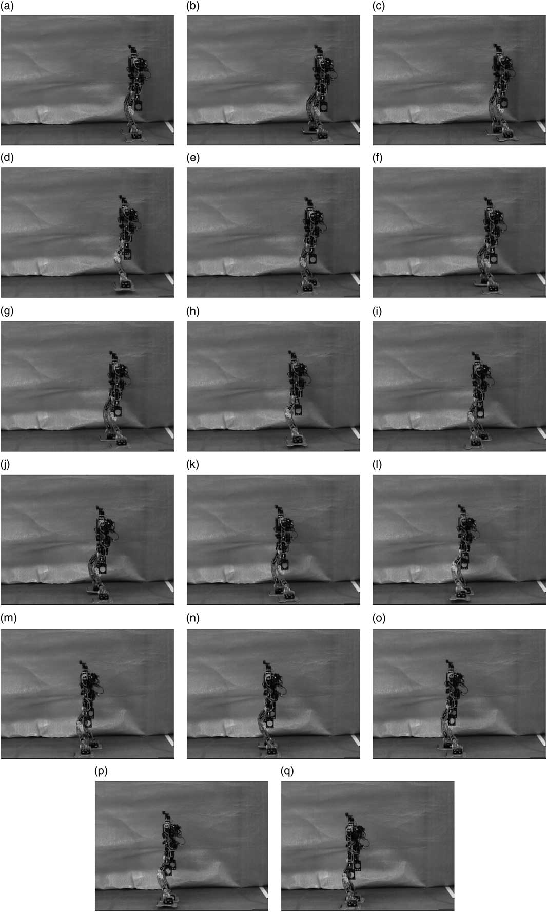
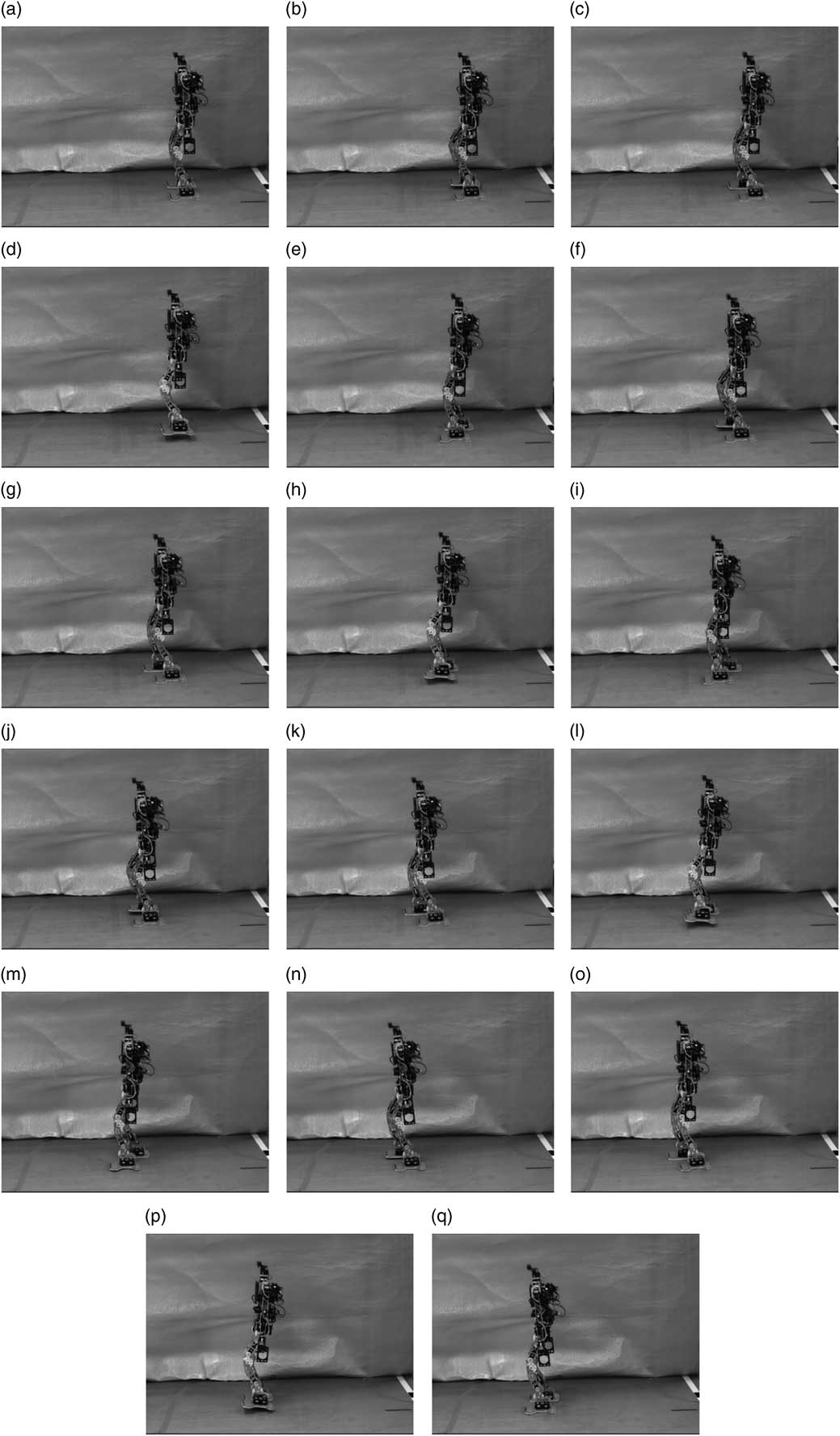
Eventually, gait patterns mentioned above were performed by David, and snapshots of both gait patterns are shown in Figure 16 (refer to the Supplementary Video 1) and Figure 17 (refer to the Supplementary Video 2), respectively. It can be seen that David Junior was able to walk stably with both gait patterns generated by using the proposed method. In addition, with gait patterns generated by using the proposed method (refer to the Supplementary Video 3), David won first place in the HuroCup sprint event at the 20th Federation of International Robot-soccer Association (FIRA) RoboWorld Cup competition, which is a well-known international robotic competition held annually. Thus, the feasibility of the proposed method has been validated.

Figure 16 Snapshots for the first gait pattern with S=[5, 5, 5, 5, 5, 5, 5, 0] cm. The robot walks stably with identical step sizes

Figure 17 Snapshots for the second gait pattern with S=[2, 2, 3, 4, 5, 4, 3, 0] cm. The robot walks stably with different step sizes
5 Conclusions
A parameterized gait pattern generator with a natural ZMP reference for biped walking has been proposed in this paper. Five types of ZMP components are presented for formulating the natural ZMP reference, and the corresponding terms for the CoM trajectory are also derived based on the relationship between ZMP and CoM from LIPM theory. Moreover, a gait planning algorithm is presented for generating a gait pattern with user-defined parameters so that parameterized gait pattern generation can be achieved. Finally, the simulation and experimental results validate the feasibility of the proposed method.
In this paper, the CoM trajectory is acquired based on a natural ZMP reference. Another factor to achieve natural walking or human-like walking may be heel-to-toe walking, which means the contact point transition of the supporting foot starts at heel-strike and ends at toe-off. Thus, extra sensors and feedback controller on the sole for achieving heel-to-toe walking can be considered as future works to enhance the walking stability and natural walking.
Acknowledgments
This work was supported in part by the Ministry of Science and Technology, Taiwan, ROC, under Grants MOST 103-2221-E-006-252 and MOST 104-2221-E-006-228-MY2, and in part by the Ministry of Education, Taiwan, within the Aim for the Top University Project through National Cheng Kung University, Tainan, Taiwan.
Supplementary Material
To view supplementary material for this article, please visit http://dx.doi.org/10.1017/S0269888916000138