


1 Introduction
RoboCup and FIRA are the leading and most diverse competitions for intelligent robots. In the humanoid league FIRA HuroCup competition, each robot must self-localize its position on the field and avoid obstacles to autonomously kick the ball to the goal, either by itself or by the help of its teammates. Therefore, a method to determine the robots’ positions and avoid obstacles is important for this competition. The FIRA field size is approximately 6 m × 5 m (child sized), bordered by a 5-cm-wide white line, and its surface is covered by green carpet, as shown in Figure 1.

Figure 1 Field of the FIRA HuroCup united soccer competition
In the humanoid robot competition, researchers (Chiang et al. Reference Chiang, Hsia, Hsu and Li2011, Reference Chiang, Hsia and Hsu2013) have applied stereo vision systems to enable a robot to self-localize its position. However, if a stereo vision system is not available for a humanoid robot, the self-localization scheme may not work as well. Some studies (Merke et al. Reference Merke, Welker and Riedmiller2004; Menegatti et al. Reference Menegatti, Pretto, Scarpa and Pagello2006, Minakata et al. Reference Minakata, Hayashibara, Ichizawa, Horiuchi, Fukuta, Fujita, Kaminaga, Irieand and Sakamoto2008) used the geometry of the field, such as the goalpost locations, in an object recognition scheme (Chiang et al. Reference Chiang, Hsia, Chang, Chang, Hsu, Tai, Li and Ho2010; Awaludin et al. Reference Awaludin, Hidayatullah, Hutahaean and Parta2013), or the white lines to calculate the position of the robot. However, goalposts have not been available in the RoboCup since 2009 and are not available in the HuroCup. As the white lines provide information regarding the field, Chiang et al. (Reference Chiang, Guo and Hu2014) proposed a white-line pattern-matching localization method for a middle-sized robot soccer game.
The white-line data from each soccer field image obtained by the robot are matched with simulated models pre-built in the database to obtain localization results. However, the white lines on the field may not be complete, and there are many similar points in the database. Thus, errors may be caused by white-line patterns extracted from the image, and the localization results will lead the robot to the wrong position. Owing to these limits as well as low reliability, localization with only white-line patterns is not suitable for actual competitions. In particular, since the robots typically face the goalposts while moving parallel to the borderlines, the white line is available only at certain locations, as shown in Figure 2. The areas marked in red indicate regions in which the white lines can be applied for the robot to self-localize. Rodriguez et al. (Reference Rodriguez, Farazi, Allgeuer, Ficht, Pavlichenko, Brandenburger, Kürsch and Behnke2018) proposed an edge detector followed by probabilistic Hough line detection to find the white line to self-localize the robot. Therefore, the white-line information plays a vital role in the soccer competition for the robot.

Figure 2 Regions in which white-line information is available
Since the gait and step of a humanoid robot can be used to determine how far a robot has moved, we designed an algorithm to integrate the gait, step, and vision system to self-localize the robot’s position. The integrated vision system is based on pattern recognition by pre-built models in the database to enhance the reliability and enable real-time processing. Furthermore, an obstacle avoidance and ball identification scheme was designed to enable the robot to move through the field and complete the tasks necessary for the united soccer competition. The remainder of this paper is structured as follows. The hardware and gait pattern are described in Section 2. The localization, obstacle avoidance, and ball identification algorithms are proposed in Section 3. The experimental results are presented in Section 4, and the paper is concluded in Section 5.
2 Hardware and gait pattern
The humanoid robot used in this study was ROBOTIS DARwIn-OP 2 (Dynamic Anthropomorphic Robot with Intelligence–Open Platform), as shown in Figure 3. This type of robot is 45.5 cm tall, which is within the required range of 40–90 cm for the child-sized humanoid RoboCup competition. The robot operates using a 1.6-GHz Intel Atom Z530 (32 bit) on-board 4-GB flash SSD, with 20 actuators, 3-axis gyroscopes, a 3-axis accelerometer, and a webcam in the head. The camera is the only sensor provided in the humanoid robot to avoid obstacles in the environment.

Figure 3 DARwIn-OP servomotor numbering and positions
The foot trajectory of a humanoid robot can be expressed by the superposition of the motion component and balance component on three axes (Ha et al. Reference Ha, Tamura and Asama2011), as defined in Equation (1). Whereas the balance component remains activated during the entire walking period, the motion component is restrained during the double-support phase (DSP). This step utilizes the parameters of amplitude  $a$, angular velocity
  $\omega $, phase shift
  $b$, offset
  $c$, and DSP ratio r and the variable A represents the movement for the three axes, X, Y, and Z. With these parameters, we can express the balance component as shown in Equation (2) and the motion component as given in Equation (3).
 $$\begin{equation}{{\rm{A}}_{\rm total}} = {{\rm{A}}_{\rm move}} + {{\rm{A}}_{\rm bal}},\end{equation}$$
 $$\begin{equation}{{\rm{A}}_{\rm bal}} = {a_{\rm bal}}{\kern 1pt} \sin ({\omega _{\rm bal}}t + {b_{\rm bal}}) + {c_{\rm bal}},\end{equation}$$
 $$\begin{align}{A_{\rm move}} = \begin{cases}{a_{\rm move}} & \left[0,\frac{rT}{4}\right)\\[3pt]{a_{\rm move}}\sin \left({\omega_{\rm move}}t + {b_{\rm move}}\right) & \left[\frac{rT}{4},\frac{T}{2} - \frac{rT}{4}\right)\\[3pt]-{a_{\rm move}} & \left[\frac{T}{2} - \frac{rT}{4},\frac{T}{2} + \frac{rT}{4}\right)\\[3pt]{a_{\rm move}}\sin \left({\omega_{\rm move}}\left(t - rT/2\right) + {b_{\rm move}}\right) & {\left[\frac{T}{2} - \frac{rT}{4}, T - \frac{rT}{4}\right)}\\[3pt]{a_{\rm move}} & \left[T - \frac{rT}{4}, T\right)\end{cases}\end{align}$$
where r = 0.25, a move_x = 30, a move_z = 30, a bal_x = 10, a bal_y = 20, and a bal_z = 3.
The foot trajectories of the robot for one step are plotted in Figures 4(a)–(c) to represent the total parameter defined in Equation (1) in X-, Y-, and Z-axis, respectively.

Figure 4 Total foot trajectory of a robot for one step
We used the foot trajectory along the X- and Y-axes for each step to calculate the moving distance in the X (left) and Y (forward) grids, resulting in a relationship between the steps and the moving distance of the robot, as shown in Figures 5(a) and (b). Linear approximation equations, plotted by red lines, are used to estimate the moving distance of the robot along the X- and Y-axes.
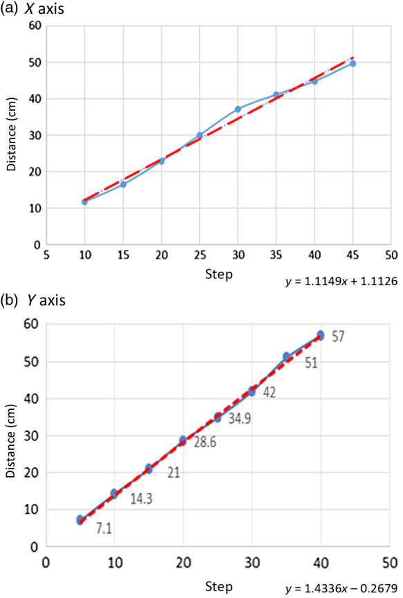
Figure 5 Relationship between steps and distances for X- and Y-axis
3 Localization and obstacle avoidance system
3.1 Localization by counting steps
To obtain the position of the robot, the 5 m × 6 m field is partitioned as a 50 × 60 grid with 10 cm × 10 cm squares, as shown in Figure 6. For example, the robot moves from one position to another, with a moving distance of d. The moving distance d and the angle θ obtained from the gyroscope are applied in Equation (4) to obtain the corresponding grid coordinates in the X and Y directions of the field. The X(t) and Y(t) coordinates are rounded to the nearest integer.

Figure 6 Grid with a 50 × 60 mesh in the X-and Y-axes for self-localization of the robot
 $$\begin{eqnarray}
X(t) & = & X(t - 1) + \left[ {dx/10 + 0.5} \right]\!,\quad X(t) \in \{0, \cdots,50\},\nonumber\\
Y(t) & = & Y(t - 1) + \left[ {dy/10 + 0.5} \right]\!,\quad Y(t) \in \{0, \cdots ,60\}.
\end{eqnarray}$$
$$\begin{eqnarray}
X(t) & = & X(t - 1) + \left[ {dx/10 + 0.5} \right]\!,\quad X(t) \in \{0, \cdots,50\},\nonumber\\
Y(t) & = & Y(t - 1) + \left[ {dy/10 + 0.5} \right]\!,\quad Y(t) \in \{0, \cdots ,60\}.
\end{eqnarray}$$
where  $dx = d\cos (\theta ),\;dy = d\sin (\theta ).$
3.2 Localization by image pattern match with a system model
Since errors may arise in the accumulated moving distance, the self-localization algorithm employs the image pattern matching with a system model to adjust the position of the robot. For the robot image, a connected-component labeling operation (He et al. Reference He, Chao, Suzuki and Wu2009) is used to distinguish the white lines, the ball, and the obstacles by assigning a unique label to each maximally connected region of foreground pixels.
In the next step, if the robot is approximately within the red dotted regions shown in Figure 2, indicating that white-line information is available for the robot, then the white-line pattern-matching algorithm is used to localize the robot’s position. As the field is divided into regions of 10 cm × 10 cm, for each region in the system model, we calculate the distance between the first white-line pixel to the bottom for all 320 scan lines from an image composed of 320 × 240 pixels, as shown in Figure 7. At grid point  ${P_M}$ in Equation (5) for the simulated system model is the ith column and jth row of the grid point, and
  $\left[ {{D_0},{\kern 1pt} {\kern 1pt} {D_1},{\kern 1pt} {\kern 1pt} {D_2}{\kern 1pt} , \cdots ,{\kern 1pt} {D_{319}}} \right]$ are the vector distances from the first white pixels to the bottom for scan line 0, 1, ⋯, 319, respectively.

Figure 7 A total of 320 scan lines are applied to calculate the distance from the first white-line pixel to the bottom
 $$\begin{equation}{P_M}({X_i},{Y_j}) = {P_{i,\kern0.7pt j}}({D_0},{\kern 1pt} {\kern 1pt} {D_1},{\kern 1pt} {\kern 1pt} {D_2}{\kern 1pt} , \cdots ,{\kern 1pt} {D_{319}})\end{equation}$$
We assume that the robot image of the field acquired by the camera corresponds to the location of P O. Then, the distances from the first white pixels to the bottom for all 320 scan lines are as follows, as shown in Equation (6):
 $$\begin{equation}{P_O}(X,Y) = P({d_0},{\kern 1pt} {\kern 1pt} {d_1},{\kern 1pt} {\kern 1pt} {d_2}{\kern 1pt} , \cdots ,{\kern 1pt} {d_{319}}),\end{equation}$$
In Equation (6),  ${d_0}$,
  ${d_1}$, ⋯,
  ${d_{319}}$ are the distances (pixels) from the first white-line pixel to the bottom for scan line 0, 1, ⋯, 319. Then, the errors for the image positions with respect to
  ${P_M}({X_i},{Y_j})$ for all grid points
  $({X_i},{Y_j})$ are defined by Equation (7).
 $$\begin{eqnarray} {E_{i,\kern0.7pt j}} & = & \left| {{P_{i,\kern0.7pt j}}({D_0},{D_1},{D_2},\cdots,{D_{319}}) - P({d_0},{d_1},{d_2},\cdots,{d_{319}})} \right|\\[4pt]& = &\left( {\sum\limits_{k = 0}^{319} {\left| {{D_k} - {d_k}} \right|} } \right)\!.\nonumber\end{eqnarray}$$
 The white-line data for each soccer field image captured by the robot are extracted and matched to simulated models in the database to obtain localization results. The location with the minimum error E i,j between the simulated model and the real field marks is the image location result  ${P_I}(X,Y)$, as shown in Equation (8).
 $$\begin{equation}{P_I}(X,Y) = \min {E_{i,\kern0.7pt j}},\end{equation}$$
where i and j are the ith column and jth row of the grid point, respectively.
To eliminate the accumulated distance error, the system model and the estimated coordinates of the robot within a range of 20 cm × 20 cm are compared in four directions (Chiang et al. Reference Chiang2016), as shown in Figure 8. Let us assume that the estimated position of the robot is within the black spot. We then use the white-line pattern on the red lines to compare the white-line pattern observed by the robot to adjust the robot position. The position with the minimum error in Equation (8) is identified as the location of the robot.

Figure 8 Comparison of the range of the system model line and the estimated robot position
3.3 Ball detection scheme
To detect the ball in soccer, the robot must have a ball identification scheme. For the ball, we used a yellow model, as shown in Figure 9. In the united soccer competition, a tennis ball is utilized for child-sized robots, and the relationship for the ball image pixel size versus distance to the robot is plotted in Figure 10. The robot uses the webcam to search for a specific model color to identify the ball and estimate its distance.

Figure 9 Ball color model

Figure 10 Relationship of the ball image pixel size versus distance to the robot
As the position of the ball is variable, we used the relative coordinates and the angle between the ball and the robot to represent the position, where the field goal is fixed at a 90-degree position, as shown in Figure 11. The robot moves around to search for the ball’s position, and the relative coordinates and the angle between the ball and the robot may vary as the robot moves, as shown in Figure 12. For example, if the ball position is in the upper-right quadrant of the robot, we obtain the angle  ${\theta _m}$, which is the angle from the line joining the two field goals to the line connecting the robot and the ball, and S, which is the distance between the robot and the ball. Then, the ball position is calculated from the relationship shown in Figure 12. We assume that
  $\phi $ is the angle that the robot has turned from facing the field goal to facing the ball. We then obtain the coordinate of the ball from Equation (9), as shown in Figure 12, where the robot has a turning angle
  $\phi $ and position (X, Y).

Figure 11 Coordinate and angle

Figure 12 Ball position at different coordinates
 $$\begin{align}
{\theta _m} &= 90^\circ - \varphi ,\quad {\rm{ball\ is\ in\ first\ quadrat}},\nonumber\\[3pt]
{\theta _m} &= \varphi - 90^\circ ,\quad {\rm{ball\ is\ in\ second\ quadrat,}}\nonumber\\[3pt]
{\theta _m} &= 270^\circ - \varphi ,\quad {\rm{ball\ is\ in\ third\ quadrat,}}\nonumber\\[3pt]
{\theta _m} &= \varphi - 270^\circ ,\quad {\rm{ball\ is\ in\ fourth\ quadrat}}.\nonumber\\[6pt]
\begin{bmatrix}
{b_{1x}}\\
{b_{2x}}\\
{b_{3x}}\\
{b_{4x}}
\end{bmatrix} &=
\begin{bmatrix}
\sin ({\theta _m})\\
- \sin ({\theta _m})\\
- \sin ({\theta _m})\\
\sin ({\theta _m})
\end{bmatrix} S + X,
\begin{bmatrix}
{b_{1y}}\\
{b_{2y}}\\
{b_{3y}}\\
{b_{4y}}
\end{bmatrix} =
\begin{bmatrix}
\cos ({\theta _m})\\
\cos ({\theta _m})\\
- \cos ({\theta _m})\\
- \cos ({\theta _m})
\end{bmatrix} S + Y,
\end{align}$$
$$\begin{align}
{\theta _m} &= 90^\circ - \varphi ,\quad {\rm{ball\ is\ in\ first\ quadrat}},\nonumber\\[3pt]
{\theta _m} &= \varphi - 90^\circ ,\quad {\rm{ball\ is\ in\ second\ quadrat,}}\nonumber\\[3pt]
{\theta _m} &= 270^\circ - \varphi ,\quad {\rm{ball\ is\ in\ third\ quadrat,}}\nonumber\\[3pt]
{\theta _m} &= \varphi - 270^\circ ,\quad {\rm{ball\ is\ in\ fourth\ quadrat}}.\nonumber\\[6pt]
\begin{bmatrix}
{b_{1x}}\\
{b_{2x}}\\
{b_{3x}}\\
{b_{4x}}
\end{bmatrix} &=
\begin{bmatrix}
\sin ({\theta _m})\\
- \sin ({\theta _m})\\
- \sin ({\theta _m})\\
\sin ({\theta _m})
\end{bmatrix} S + X,
\begin{bmatrix}
{b_{1y}}\\
{b_{2y}}\\
{b_{3y}}\\
{b_{4y}}
\end{bmatrix} =
\begin{bmatrix}
\cos ({\theta _m})\\
\cos ({\theta _m})\\
- \cos ({\theta _m})\\
- \cos ({\theta _m})
\end{bmatrix} S + Y,
\end{align}$$
where (b ix, b iy) is the ball position in the ith quadrant, i = 1, …, 4.
3.4 Obstacle avoidance system
An obstacle avoidance technique was proposed by Chiang (Reference Chiang2016). For this method, the image is transformed into a binary image, where obstacles are indicated as black pixels. Then, image preprocessing techniques, such as dilation and elution, are applied, and the image is reduced to a 32 × 24 grid of 10 × 10 pixel squares (Hsia et al. 2012). The depth vector D is defined in Equation (10) as a 1 × 32-dimensional vector, where each dimension is the distance from the first obstacle’s location to the bottom-row location for one column.
 $$\begin{equation}D = \left[ {{d_1},{d_2}, \cdots ,{d_{32}}} \right]\!,\end{equation}$$
where d i is the distance from the first black grid location to the bottom row for the ith column.
To prevent the robot from hitting the obstacle, the focus area in front of the robot, as shown in Figure 13, is defined in Equation (11).
 $$\begin{equation}F = \left[ {{f_1},{f_2}, \cdots \kern-1pt,{f_{32}}} \right]\!,\end{equation}$$

Figure 13 Focus area and the distances of the obstacle, d y and d x
where
 $$\begin{equation*}{f_i} =
\begin{cases}
i, & 1 \le i \le 16\\[2.5pt]
33 - i, & 16 < i \le 32
\end{cases}
\end{equation*}$$
$$\begin{equation*}{f_i} =
\begin{cases}
i, & 1 \le i \le 16\\[2.5pt]
33 - i, & 16 < i \le 32
\end{cases}
\end{equation*}$$
To verify whether an obstacle is within the focus area, the vector V is defined in Equation (12). If V is not equal to 0, the obstacle is within the focus area; thus, the robot should move.
 $$\begin{equation}V = \left[ {{v_1},{v_2}, \cdots ,{v_{32}}} \right],\end{equation}$$
Weighting factors are defined in Equations (13) and (14) to determine the direction in which the robot should move. If W L is greater than W R, the robot will move to the left, and the boundary point x b will be set to be the farthest right point, 319. Otherwise, the robot will move to the right, and the boundary point x b will be set to be the farthest left point, 0. The boundary point x b is defined in Equation (15).
 $$\begin{equation}{W_R} = \sum\nolimits_{i = 1}^{32} {(33 - i)} \times {v_i}\end{equation}$$
 $$\begin{equation}{W_L} = \sum\nolimits_{i = 1}^{32} i \times {v_i}\end{equation}$$
 $$\begin{equation}{x_b} = \begin{cases}0,& {W_L} \le {W_R}\\319,&{W_L} > {W_R}\end{cases}\end{equation}$$
To obtain the minimal distance from the robot to the obstacle, we have the boundary distance in the Y direction, d y, defined in Equation (16) as the shortest distance among the values in vector D. The distance d x defined in Equation (18) is the distance from the center point of the obstacle x c, defined in Equation (17), to the boundary point x b in the X direction. The d y and d x curves shown in Figure 13 present the minimum distance of the obstacle in the vertical direction and the distance from the center of the obstacle to the horizontal boundary, respectively. These two parameters are used in the fuzzy logic control system to determine the movement of the robot for obstacle avoidance.
 $$\begin{equation}{d_y} = \min \{ {d_i}\} \end{equation}$$
 $$\begin{equation}{x_c} = \left({\sum\nolimits_{i = 1}^n {{x_i}} }\right)/n,\quad ({x_i},{y_i}) \in A \end{equation}$$
Here, A is a region in which obstacles are within the focus area, and n grids are assumed in the focus area.
 $$\begin{equation}{d_x} = \left| {{x_c} - {x_b}} \right|\end{equation}$$
The fuzzy rule is used to modify the speed (forward) and turning (horizontal) movement of the robot, based on the distances d x and d y for obstacle avoidance based on a vision system.
4 Experimental results
In this section, experiments are reported for localization based on the step and distance relationship and for localization based on white-line pattern matching to verify the performance of the proposed localization scheme. The obstacle avoidance and ball identification schemes are integrated as a ball tracing and kicking motion.
4.1 Localization by counting steps
The experiment is initiated from the bottom line of the field to evaluate the accuracy of the localization method based on counting steps, and the results are shown in Table 1. The counting steps can provide a reasonable accuracy for localization within a distance of 90 cm.
Table 1 Positioning by counting steps

Next, five test points located beyond 90 cm, as shown in Figure 14, are applied to evaluate the localization method based on counting steps. The robot started from the center of the defense area and walked to the test points, with the results listed in Table 2. The error is determined using the grid coordinates defined in Section 2.2. The results showed that the localization error for closer positions, that is, test points 4 and 5, corresponds to approximately one grid distance for the X-axis and two grid distances for the Y-axis. However, the error accumulates as the robot walks to farther positions, that is, test points 1 and 2, with errors of approximately two grid distances for the X-axis and five grid distances for the Y-axis. These results demonstrate that the localization method based on step counting works well only for test points close to the starting point, while greater distances result in a high accumulated error.

Figure 14 Five test points to verify the localization method based on step counting
Table 2 Positioning by step counting

4.2 Localization by image pattern match with a system model
To adjust the accumulated error caused by step counting, we also performed localization by image pattern matching with a system model. Experiments were performed three times at different positions, as shown in Figures 15–17. In these figures, the left image presents the position of the robot and the right image presents the image patterns visualized by the robot. The position results are summarized in Table 3. The image pattern matching and step counting methods were implemented as follows. The first robot position is obtained by step counting. Then, the robot uses image pattern matching with the system model to compare the white-line information with the pattern over 20 cm, as shown in Figure 8, to determine the most suitable position to minimize the accumulated error. As shown in Table 3, the estimated positions determined by image pattern matching have a smaller error than those obtained by step counting for distances of 10–20 cm.

Figure 15 Exp. 1 for localization by image pattern matching with system model

Figure 16 Exp. 2 for localization by image pattern matching with system model

Figure 17 Exp. 3 for localization by image pattern matching with system model
Table 3 Positioning by image pattern matching

4.3 Obstacle avoidance and ball kicking scheme
To verify the obstacle avoidance and ball kicking scheme, further experiments were performed, with the results shown in Figure 18. The robot started from the center of the defense area, as shown in Figure 18(a), to locate the ball while avoiding obstacles on the field. As shown in Figures 18(b)–(h), the robot can avoid obstacles while locating the ball and kicking the ball to the goal.

Figure 18 The robot avoids the obstacles and kicks the ball to the goal
5 Conclusions
In this study, we designed a localization and obstacle avoidance system integrated with a ball identification scheme for the FIRA competition. The localization is implemented by combining the grid points, gait, and steps to determine the position of each robot. To enhance the localization accuracy and reduce the accumulated error induced by step counting, a localization method based on image pattern matching with a system model is implemented. The system also enables the robot to locate the ball on the field using a color model of the ball and avoid obstacles by calculating the obstacle distance based on data extracted from real-time images. The proposed algorithm exhibits an error of 20 cm or less, and the localization scheme is practical for implementation in a robot soccer competition. With the integration of an accurate self-localization algorithm, ball identification scheme, and obstacle avoidance system, the robots are capable of accomplishing the tasks necessary for a soccer competition.


