


I. Introduction and Literature
In the hedonic price approach, the price of a good or service is split into several implied prices that relate to specific characteristics of a good or service for which consumers are willing to pay. In the most common application of the hedonic approach to analyzing wine prices, a log-linear regression is used to estimate the price

where P is a price vector of a 0.75 liter bottle of wine, X denotes a matrix of characteristics which are supposed to have an influence on the wine price, β is the vector of parameters that are associated to these characteristics, and ɛ is the error term (Thrane, Reference Thrane2004).
There is a growing number of studies dealing with the impact of weather changes on wine quality and wine prices.Footnote 1 Most of these studies suggest that temperature and precipitation during the growing and harvesting seasons may have an important impact on wine prices (e.g., Ashenfelter, Reference Ashenfelter2010; Ashenfelter and Storchmann, Reference Ashenfelter and Storchmann2010; Byron and Ashenfelter, Reference Byron and Ashenfelter1995; Haeger and Storchmann, Reference Haeger and Storchmann2006; Jones and Storchmann, Reference Jones and Storchmann2001; Lecocq and Visser, Reference Lecocq and Visser2006; Oczkowski, Reference Oczkowski2001, Reference Oczkowski2014, Reference Oczkowski2016; Ramirez, Reference Ramirez2008; Storchmann, Reference Storchmann2005, Reference Storchmann2012). As weather information is not given on the wine label, visible quality indicators include the quality categories or the alcohol level as direct measures of quality that are affected by weather (Niklas, Reference Niklas2017), and wine guide scores as indirect measures of wine quality (Schamel, Reference Schamel2000, Reference Schamel2002, Reference Schamel2003; Shapiro, Reference Shapiro1983; Tirole, Reference Tirole1996).
Most of the extant studies use either time series data or cross-sectional data and apply (log)linear regression approaches to identify the impact of the weather, while other disciplines such as engineering or stock exchange trading use machine learning (Shavlik and Diettrich, Reference Shavlik and Diettrich1990) as the core technology for their model building capabilities (Stone et al., Reference Stone, Brooks, Brynjolfsson, Calo, Etzioni, Hager, Hirschberg, Kalyanakrishnan, Kamar, Kraus, Leyton-Brown, Parkes, Press, Saxenian, Shah, Tambe and Teller2016).Footnote 2 There is only one paper to date, that deals with the prediction of wine prices applying machine learning. This paper focuses on time-series analyses required for stock exchange trading (Yeo, Fletcher, and Shawe-Taylor, Reference Yeo, Fletcher and Shawe-Taylor2015).
The current study focuses on separate equations for different German grape varieties, assuming that these grape varieties react differently to weather variables. The results of the log linear regression (and squared forms) and the machine learning are first compared for the Riesling grape variety, then the machine learning is applied for the other grape varieties.
The article is organized as follows. Section II presents the data. Section III describes the methodological approach. Section IV reports the results and Section V draws conclusions.
II. Data on German Weather and Wine Prices
We base our analysis on a dataset that covers farm gate prices for 0.75 liter bottles of wine,Footnote 3 reported by 177 wine producers that we sampled at random for the Riesling, Silvaner, Pinot Blanc, and Pinot Noir grape varieties for the vintages 1998 to 2013, for all 13 German wine regions. We obtained farm gate pricesFootnote 4 from these producers with data on various control variables from “Gault&Millau Weineguide Deutschland” (Diel and Payne, Reference Diel and Payne2002–2009; Payne, Reference Payne2010–2015). Table 1 summarizes all collected variables for the Riesling grape variety.Footnote 5
Table 1 Descriptive Statistics for Riesling
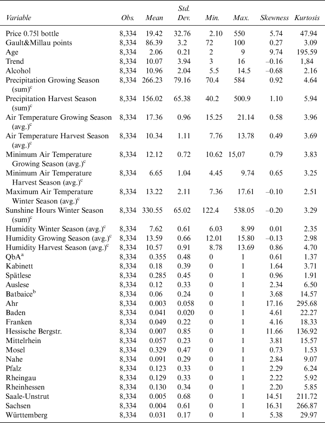
a QbA: Qualitätswein
b Batbaice: Beerenauslese/Trockenbeerenauslese/Eiswein
c Winter Season: 12/01–02/28; Growing Season: 03/01–09/15; Harvest Season: 09/16–10/31
Source: Authors’ calculations.
We use German quality categories as direct measures of quality. German wines are categorized by the degree of ripeness of the grapes, measured as the content of natural sugar in the must (grape juice) at harvest. However, these so called “quality categories” do not measure, per se, whether a wine is of good or bad quality.Footnote 6 The German term is “degree Oechsle”Footnote 7 and the following categories are distinguished: Qualitätswein (QbA),Footnote 8 Kabinett, Spätlese, Auslese, Beerenauslese, Trockenbeerenauslese, and EisweinFootnote 9 (Ashenfelter and Storchmann, Reference Ashenfelter and Storchmann2010).
Instead of collecting data from a single weather station, as shown in the literature (Lecocq and Visser, Reference Lecocq and Visser2006; Haeger and Storchmann, Reference Haeger and Storchmann2006), this study uses daily data (daily average temperature,Footnote 10 average of the daily maximum and daily minimum temperature all in degrees Celsius, sum of precipitation in mm, and daily average humidity in percent) from 13 different local weather stations,Footnote 11 as especially since precipitation varies between German wine regions, which therefore differ in their suitability for grape growing, while one weather station would have been suitable in the case of the temperature due to spatial correlation (Ashenfelter and Storchmann, Reference Ashenfelter and Storchmann2010; Haeger and Storchmann, Reference Haeger and Storchmann2006). Overall, our sample comprises 8,334 observations for Riesling, 2,004 for Pinot Noir, 1,294 for Pinot Blanc, and 917 for Silvaner.
Mainly the regions Mosel (32.9%), Pfalz (12.3%), Rheingau (12.9%), and Rheinhessen (13%) produce Riesling and the quality categories are QbA (35.5%), Spätlese (28.5%), Kabinett (18%), Auslese (12%), and Beerenauslese/Trockenbeerenauslese/Eiswein (Batbaice) (6%). The price of Riesling varies tremendously, from €2.10 to €550.00 per bottle, while Gault&Millau quality points vary between 72 and 100.
III. Methods
In the first step, we run a log linear regression for Riesling and follow the variables employed in the previous literature. The hedonic equation is

where GMP denotes Gault&Millau points (as an indirect measure of quality), age is the age of the wine at the time of purchase, trend is an annual trend variable to capture inflationary trends, W4 ... Wk are various weather variables (average air temperature, squared temperature, sum of precipitation in mm) which we split into the growing and harvest seasons,Footnote 12 Quality is a series of dummy variables for the German quality categories (as a direct measure of quality), Region is a series of dummy variables depicting the region from where the grapes are sourced, and Producer is a series of dummy variables reflecting price policies and other farm specific factors (production cost, capital cost, owner structure, etc.).
In the second step, we substitute the log linear regression algorithm with machine learning (Witten, Eibe, and Hall, Reference Witten, Eibe and Hall2017). We build a non-linear regression model including all variables, which uses a classic feed forward artificial neural network (ANN) algorithm (Witten, Eibe, and Hall, Reference Witten, Eibe and Hall2017; Hornik, Stichcombe, and White, Reference Hornik, Stichcombe and White1990; Rumelhart, Hinton, and Williams, Reference Rumelhart, Hinton and Williams1986) to generate the functional model between environmental and other variables related to logarithmic bottle prices.
An ANN is a mathematical simulation of the biological nervous cell system and consists of many regression units, which are typically non-linear, but could also be linear for scaling purposes. These units are also known in the literature as perceptrons (Rosenblatt, Reference Rosenblatt1958), neurons, or nodes and are organized in layers (Witten, Eibe, and Hall, Reference Witten, Eibe and Hall2017; Hornik, Stichcombe, and White, Reference Hornik, Stichcombe and White1990; Rumelhart, Hinton, and Williams, Reference Rumelhart, Hinton and Williams1986). Each layer is stacked on top of the other and all nodes of the underlying layer have a direct weighted link to each unit in the following layer. Several kinds of architecture exist, where the layers can be skipped or where there are feedback loops between previous layers (Witten, Eibe, and Hall, Reference Witten, Eibe and Hall2017). Feed forward networks, those without any feedback loops or recursions, typically have three types of layers. The input layer type that uses the values of the independent variables as input, the hidden layer type that is responsible for the non-linear functional regression, and the output layer type that performs the final transformation to the dependent variables. Equation (3) describes the general form of the network architecture as

where x i is an independent variable and fi is the transfer function on the input layer, fh is the transfer function of the hidden layer, and fo is the transfer function of the output layer. The transfer function in this case is the logistic sigmoidal function as described in Equation (4).

In the third step, we calculate the dependency matrix (Rinke, Reference Rinke2015) for the previously generated ANN model. We derive the dependency matrix from a sensitivity analyses of the ANN model, which Hashem (Reference Hashem1992) originally presented and Yeh and Cheng (Reference Yeh and Cheng2010) further investigated. It represents a normalized, accumulated Jacobi matrix (Rudin, Reference Rudin1976) over the observed data samples and expresses the relative importance of an independent variable with respect to the dependent variable of the ANN model.
There are two other methods of describing the “importance” of an independent variable with respect to the dependent variable, but these are based only on the learned internal network weights w ij (Olden and Jackson, Reference Olden and Jackson2002; Olden, Joy, and Death, Reference Olden, Joy and Death2004; Garson, Reference Garson1991; Goh, Reference Goh1995; Giam and Olden, Reference Giam and Olden2015). Yeh and Cheng (Reference Yeh and Cheng2010) show that calculating importance as a value, based on the first order partial derivative and further on, the second order partial derivative is more accurate than other common methods.
We calculate the dependency factor (Rinke, Reference Rinke2015) for each independent variable of the model with respect to the dependent variable separately using Equation (5). Yeh and Cheng (Reference Yeh and Cheng2010) call this dependency factor the “average linear importance factor”

where ${{\partial y} \over {\partial x}}$ represents the partial derivative of the function y(x) and n the number of samples.
In addition to the dependency factors, we examine the semi-elasticity ε of y(x) (Owen, Reference Owen2012). Semi-elasticity measures the percentage change in the dependent variable caused by a unit change in the independent variable. In the log-linear-regression model log(y) = ß 0 + ß 1x + u. The variable ß 1 measures the semi-elasticity of the dependent variable in relation to the respective independent variable. Since we use a log-linear specification between the log-price and an independent variable x, a change of one unit of x results in an ε × 100 percent change in y.Footnote 13 We calculate the semi-elasticity following Equation (6) and the average semi-elasticity following Equation (7).


for n observations
In the fourth step, we calculate the average semi-elasticity for each independent variable of the model with respect to the dependent variable separately for each German quality category (QbA, Kabinett, Spätlese, Auslese, and Batbaice) and discuss the results. For the remaining grape varieties, Silvaner, Pinot Blanc, and Pinot Noir, we repeat steps two to four and summarize the results (only available online).
IV. Results
A. Riesling Models
(1) Log Linear Regression
We apply the hedonic Equation (2) using average temperature functions for the growing and harvest seasons in Model 1, squared temperature functions in Model 2, and omitting Gault&Millau points in Model 3 applying robust standard errors.Footnote 14
The reason for using squared temperatures in Model 2 is to check for non-linear temperature effects. The Gault&Millau points are omitted in Model 3 to check whether the weather variables can cover most quality aspects. The results are shown in Table 2 with an R2 of 0.7974 (Model 1), 0.7979 (Model 2), and 0.6168 (Model 3).Footnote 15
Table 2 Comparison of Model 1, 2, and 3 for Riesling (without Regional and Producer Fixed Effects)
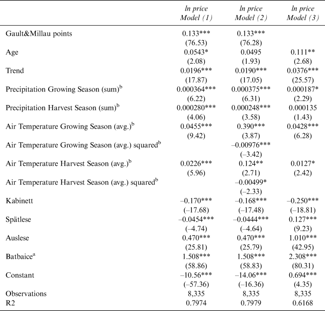
Note: Robust t statistics are in parentheses; significance levels are *p < 0.05, **p < 0.01, and ***p < 0.00.
a Batbaice: Beerenauslese/Trockenbeerenauslese/Eiswein
b Winter Season: 12/01–02/28; Growing Season: 03/01–09/15; Harvest Season: 09/16–10/31
Source: Authors’ calculations.
All significant weather variables show a positive impact on wine prices in all three models. Model 3 suggests that average temperatures during the growing and harvest seasons have a significantly positive but decreasing effect, because the squared functions are negative. Based on these results, we calculate the price-maximizing temperature, which is 19.98 degrees Celsius for the growing season and 12.42 degrees Celsius for the harvest season.
Gault&Millau points have the greatest influence on the Riesling price, as the price increases by 13.3% with each additional point in Models 1 and 2. The exclusion of Gault&Millau points leads to less accurate results and a much lower R2.
The price trend has a significantly positive impact in all three models (between 1.9% and 3.76%) and the wine price increases with the age of the wine by 5.43% in Model 1 and 11.1% in Model 3, but is insignificant in Model 2.
Quality categories also have a significant impact. Compared to QbA, the Kabinett category leads to a decline in prices for all three models and Spätlese leads to a decline in prices for Models 1 and 2, while the higher-quality categories lead to much higher prices. The quality Auslese category has a positive price impact from 47% (Models 1 and 2) to 101% (Model 3), and Batbaice from 150.8% (Models 1 and 2) to 230.8% (Model 3).
We then estimate the above models applying regional fixed effects to control regional unobserved heterogeneity. Table 3 (left side) shows the results with an R2 of 0.8020 (Model 4), 0.8020 (Model 5), and 0.6348 (Model 6).
Table 3 Models for Riesling
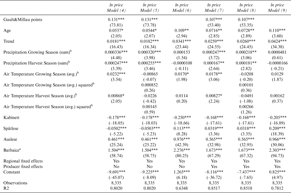
Note: Robust t statistics are in parentheses; significance levels are *p < 0.05, **p < 0.01, and ***p < 0.00.
a Batbaice: Beerenauslese/Trockenbeerenauslese/Eiswein
b Winter Season: 12/01–02/28; Growing Season: 03/01–09/15; Harvest Season: 09/16–10/31
Source: Authors' calculations.
While most of the results are confirmed, Model 5 shows the most obvious change in results. Including squared temperature variables now makes all temperature variables insignificant. One reason might be that non-linear temperature effects are only observed in some regions, so the effects are no longer significant when we apply regional fixed effects. We confirm this assumption when running regressions for regional subsamples: squared temperature variables for both the growing and harvest seasons are only significant for the regions of Baden (in the very south of Germany) and for Mittelrhein (a sunny wine region), while for the harvest season squared temperature variables are only significant for the regions of Nahe and Württemberg (again, in the very south of Germany). The majority of observations (6,504 out of 8,335), however, cover German wine regions with linear temperature effects. Model 6 again has less accurate results than the other two models.
Finally, we estimate the same models applying regional and producer fixed effects that can reflect pricing policies and other farm-specific factors such as production cost, capital cost, or owner structure. Table 3 (right side) shows the results, with an R2 of 0.8517 (Model 7), 0.8518 (Model 8), and 0.7812 (Model 9).
The application of producer fixed effects generally leads to a higher explanatory power of all models. The effect of Gault&Millau points is less strong than before (10.7% instead of 13.1%), while age and trend have stronger effects. Only in Model 7 do all weather variables show a significant and positive effect on wine prices, while the inclusion of squared temperature effects still leads to insignificant results. Similar to the previous explanation, this may be due to the majority of producers in this sample (74.1%) are in regions with linear temperature effects according to the regional subsamples.
Due to the high degree of skewness (5.74) and kurtosis (47.94) in the price data (see Table 1), we assume that marginal effects might vary in different price brackets. Therefore, we finally run a quantile regression for Model 4 (with regional fixed effects without squared temperaturesFootnote 16) and report the results and the corresponding ordinary least square (OLS) results in Table 4 (Column 1), allowing for a direct comparison of results.
Table 4 OLS vs. Quantile Regressions of Model 4 for Riesling

Note: All equations include a full set of regional fixed effects. Robust t statistics are in parentheses; significance levels are *p < 0.05, **p < 0.01, and ***p < 0.00.
a Batbaice: Beerenauslese/Trockenbeerenauslese/Eiswein
b Winter Season: 12/01–02/28; Growing Season: 03/01–09/15; Harvest Season: 09/16–10/31
Source: Authors’ calculations.
Similar to the OLS results, Gault&Millau points have a positive affect on the price. The effect peaks in the 0.75 quantile and then decreases slightly afterwards.
The age of a wine bottle, which is statistically significant in the OLS regression, only exerts a significantly positive price effect in the 0.5 quantile and remains insignificant for all others.
The quantile regression shows significant trend effects like the OLS, but the trend effect decreases with the price quantiles.
Like in the OLS results, wine prices in the growing season are significantly positively affected by precipitation, with a peak in the 0.25 quantile. Precipitation in the harvest season only has a significant positive price effect in the 0.25 quantile and then again in the 0.75 and 0.9 quantiles, the effect increasing with the price quantiles.
The average temperature in the growing season shows a significantly positive price effect only for the 0.25 and 0.5 quantiles, with a peak for the 0.25 quantile. The same holds to the average temperature in the harvest season, which is significantly positive for the 0.9 quantile.
The highest German quality categories, Auslese and Batbaice, show a highly significant positive effect on wine prices. This effect increases with the price quantiles and accounts for a price increase of up to 61% for Auslese and up to 171.1% for Batbaice.
The Kabinett category shows no significant effect for the 0.25 quantile, but for all other quantiles there is an increasing, significantly negative effect on wine prices. For Spätlese, the effect is significantly positive for the 0.25 quantile, but significantly negative for the quantiles 0.5, 0.75, and 0.9.
(2) Machine Learning Approach
All available variables (see Table 1) can be used for the application of ANNsFootnote 17 without a negative impact on the model accuracy, since ANN models are robust with regard to multicollinearity (Dumancas and A Bello, Reference Dumancas and A Bello2015; Garg and Tai, Reference Garg and Tai2013).
First, we investigate a feasible architecture for the ANN model that matches the Riesling dataset. As a result of several experiments with different architectures and the intention to maximize the R2, to minimize root mean squared error (RMSE) and to avoid overfitting, we found a four-layer architecture for the Riesling model. Thus, all 44 input variables, including quality fixed effects and regional fixed effects and, therefore, 44 nodes in the input-layer, 15 nodes in the first hidden layer and one node in the second hidden layer, and finally one output node for our dependent variable. In the next step, we train the Riesling model and calculate the dependency matrix and the semi-elasticity, which gives a sextuple for each independent variable, applying quality fixed effects.
We interpret a variable as important (significant) and influential if it has a high dependency value and a high semi-elasticity value.Footnote 18 Table 5 shows the significant and influential variables for Riesling.Footnote 19 We additionally include Humidity as an independent variable because it has rarely been used in the literature.
Table 5 Significant and Influential Variables for Riesling
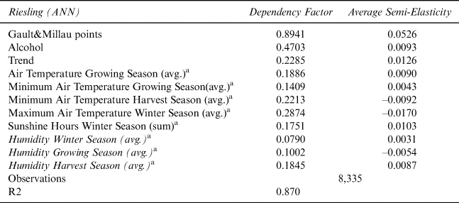
a Winter Season: 12/01–02/28; Growing Season: 03/01–09/15; Harvest Season: 09/16–10/31
Source: Authors’ calculations.
The ANN model is of higher explanatory power as it is possible to also capture non-linear relationships,Footnote 20 and the resulting R2 is now 0.876. Furthermore, the RMSE with a value of 0.293 shows a better model accuracy (about 18.7% better) than the log linear regression model.
Again, we identify Gault&Millau points as the most important (nonfixed effect) variable with a dependency factor of 0.894, which also shows the highest semi-elasticity, with a price increase of 5.26% for each additional Gault&Millau point.
Like in the log linear regression model, there is a positive price trend, while the age of the wine does not seem to be important for the Riesling prices. The average (and also minimum) temperatures in the growing season again have a positive influence on wine prices, while precipitation does not seem to be relevant.
Some additional variables exert a price effect. The alcohol level has a positive effect on the price, while the rise in the maximum temperatures in the winter season and the minimum temperatures in the harvest season have negative prices effects, so that an increase in extreme weather conditions is, therefore, unfavorable for Riesling.
The ANN model allows the semi-elasticity to be split for each independent variable into a semi-elasticity per fixed effect (here the respective quality category), which improves the interpretation of the results. Table 6 shows the splitting into these semi-elasticities per quality category for Riesling.
Table 6 Average Semi-Elasticity of Significant and Influential Variables for Riesling by Quality Category

a Winter Season: 12/01–02/28; Growing Season: 03/01–09/15; Harvest Season: 09/16–10/31
b Qualitätswein
c Batbaice: Beerenauslese/Trockenbeerenauslese/Eiswein
Source: Authors’ calculations.
The very left column of Table 6 shows the average coefficient (semi-elasticity), while the other 5 columns show the semi-elasticity per quality category. Here, the influence of additional Gault&Millau points on the price for QbA wines (+7.41%) is very high, but only small for wines of the Kabinett quality (+2.67%) and medium for Spätlese (+4.28%), Auslese (+5.85%), and Batbaice (+4.05%). Table 6 shows the positive influence of the alcohol level on the prices of QbA wines (+3.68%), Kabinett (+0.17%), and Spätlese (+0.63%), while the impact is negative regarding the prices of wines of the quality categories Auslese (–3.29%) and Batbaice (–3.02%). A rise in maximum temperatures during the winter season is not favorable for all quality categories of Riesling.
With the scatter plots in Figures 1 and 2, we further split the semi-elasticities and distinguish between the influence on low- and high-priced wines within a single quality category.

Figure 1 Average Semi-Elasticity of Gault&Millau Points for Each Riesling Quality Category
Source: Authors’ calculations.
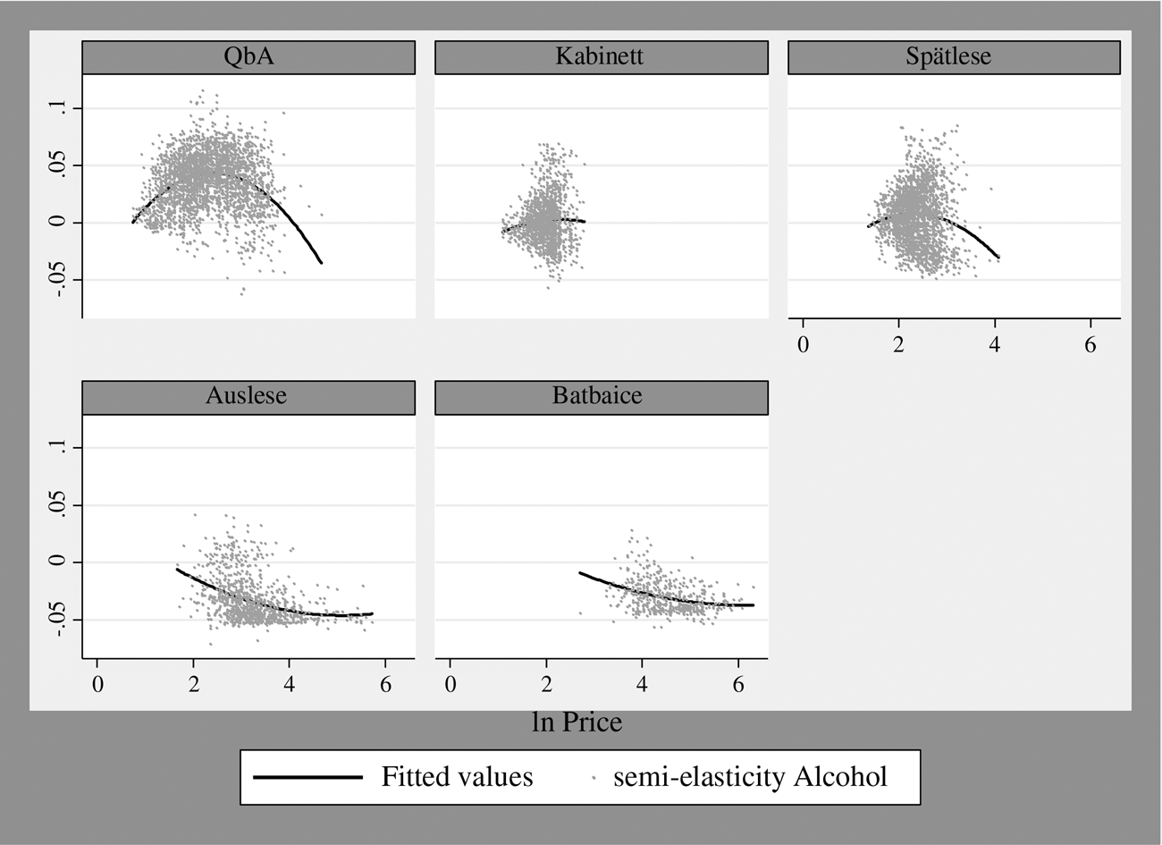
Figure 2 Average Semi-Elasticity of the Alcohol Level for Each Riesling Quality Category
Source: Authors’ calculations.
Figure 1 shows that wines with a lower QbA benefit from additional Gault&Millau points, while wines with a higher price do not. This is the opposite for all other quality categories, since the higher the price, the more positive the price effect.
Figure 2 shows that the influence of the alcohol level is higher for QbA wines with lower prices than for QbA wines with higher prices, and that there is a slightly positive effect on higher-priced Kabinett wines. The scatterplot clearly confirms the negative influence of higher alcohol percentages on wine prices for the quality categories Spätlese, Auslese, and Batbaice.
B. ANN Regression Models for Silvaner, Pinot Blanc, and Pinot Noir
We also conduct the analysis for the Silvaner, Pinot Blanc, and Pinot Noir grape varieties, but as mentioned in Section III, we exclusively apply the machine learning approach due to its better performance. We again build an ANN and apply the same architecture as used for the Riesling model in order to compare the results.
Table 7 shows the dependency matrix and average semi-elasticities for the most important and influential variables for the other three grape varieties.Footnote 21
Table 7 Dependency Matrix and Average Semi-Elasticity for Silvaner, Pinot Blanc, and Pinot Noir
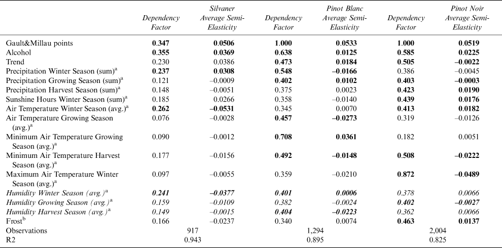
Note: Significant and influential variables for each grape variety in bold letters.
a Winter Season: 12/01–02/28; Growing Season: 03/01–09/15; Harvest Season: 09/15–10/31
b Frost: Sum of days of frost, with soil temperatures < 0 during winter, growing, and harvest seasons.
Source: Authors’ calculations.
Figure 3 (dependency factor) and Figure 4 (average semi-elasticity) visualize the differences between grape varieties regarding dependency factors and average semi-elasticities more easily for all grape varieties, including Riesling.

Figure 3 Dependency Factors for Riesling, Silvaner, Pinot Blanc, and Pinot Noir
Source: Authors’ calculations.

Figure 4 Average Semi-Elasticity for Riesling, Silvaner, Pinot Blanc, and Pinot Noir
Source: Authors’ calculations.
Regarding the dependency factors, Figure 3 clearly shows that the “Gault&Millau points” is the most important independent variable for the prices of all grape varieties and that the various weather variables have differing levels of importance for these prices with the variable “maximum air temperature in the winter season” being the most important one for Pinot Noir prices, and the variable “minimum air temperature in the growing season” for Pinot Blanc prices.
The same applies to the average semi-elasticities (Figure 4) with “Gault&Millau points” and on a lower level “Alcohol” as variables with a highly positive influence on the prices of all grape varieties, the variable “minimum air temperature in the growing season” having a highly positive effect on Pinot Blanc prices, the “air temperature in the winter season” having a highly negative effect on Silvaner prices, and “maximum air temperature in the winter season” on Pinot Noir prices.
We calculate the semi-elasticities per quality category of important (significant) and influential variables for Silvaner, Pinot Blanc, and Pinot Noir as we did for Riesling. The respective scatter plots show whether there is a difference between lower- and higher-priced wines in each quality category for each independent variable.
These results are only addressed in the online publication.
V. Conclusion
The results suggest that a simple hedonic price equation does not exist for all grape varieties. It is more appropriate to use different price equations for each grape variety. The log linear regression model for Riesling finds positive effects especially of Gault&Millau points, but also of age, trend, and average temperatures as well as precipitation on German wine prices. The quality categories Auslese and Batbaice lead to very high-price premiums for Riesling. The non-linear regression using ANNs performs slightly better than the log linear regression model because it delivers better results with respect to R2 and RMSE, suggests some additional explanatory variables (such as alcohol level or minimum and maximum temperatures), and gives a more detailed insight into the interpretation of explanatory variables.
Therefore, the results for Silvaner, Pinot Blanc, and Pinot Noir are based on the machine learning approach. It is shown that the influence of an independent variable on the wine price of a certain grape variety cannot be estimated by a single coefficient, since the influence clearly differs for each quality category (fixed effect) of the respective wine.
The results of the machine learning model also suggest that Gault&Millau points have a significant and high influence on German wine prices, as one additional point increases wine prices by around 5% regarding the average coefficients, but with differences between quality categories. The split analysis shows that the lowest German quality category QbA has the highest premiums, while the highest quality category Batbaice only has high premiums for Pinot Noir. Additional scatter plots show that the higher-priced QbA wines benefit more from additional Gault&Millau points than the lower-priced QbA wines.
The influence of the alcohol level on wine prices is positive with regard to the average coefficient, but the split analysis shows that this influence holds especially to the quality categories QbA, Kabinett, and Spätlese and that the influence is even negative for the quality categories Auslese (except for Pinot Noir) and Batbaice (except for Pinot Blanc).
There are essential differences between grape varieties regarding influential weather variables and their ability to cope with rising temperatures or extreme weather (minimum and maximum temperatures) in different seasons of the ripening process.
Rising average air temperatures during the winter season lead to a decrease in prices for Riesling and Silvaner, while Pinot Blanc copes better with rising winter temperatures and Pinot Noir, the only red variety in the sample, even shows a positive effect of both the rising minimum and average temperatures, but all varieties cannot cope with rising maximum temperatures in the winter season.
During the harvest season, especially higher minimum and maximum temperatures lead to a negative price effect for wines of all grape varieties and quality categories, so that earlier harvest is recommended for all grape varieties in cases of warmer harvest seasons, such as was the case in 2018.
Precipitation does not seem to have as high an impact but is different for each grape variety and quality category.
In the analysis, ripeness levels are used as proxies for quality levels according to the German classification system. Future research may include investigating the effects of climate change on wine prices from regions with distinct quality levels, such as Bordeaux.
Supplementary Material
To view supplementary material for this article, please visit https://doi.org/10.1017/jwe.2020.16.
Appendix
Table A1 Correlation Matrix Between Gault&Millau Points and German Quality Categories

Table A2 Breusch–Pagan/Cook–Weisberg Test for Heteroskedasticity – Model 1, 2, and 3
Breusch–Pagan/Cook–Weisberg test for heteroskedasticity
Ho: Constant variance
Variables: fittes values of logprice075

Table A3 Variance Inflation Tests for Multicollinearity for Model 1, 2, and 3
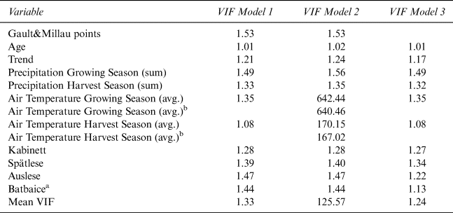
Table A4 Correlation Matrix for Model 1


