


Introduction
Allometric relationships enable the estimation of above-ground biomass of trees from structural measurements (e.g. diameter, height, crown breadth; Chave et al. Reference Chave, Andalo, Brown, Cairns, Chambers, Eamus, Fölster, Fromard, Higuchi, Kira and Lescure2005, Henry et al. Reference Henry, Picard, Trotta, Manlay, Valentini, Bernoux and Saint André2011, Pastor et al. Reference Pastor, Aber and Melillo1984, Young et al. Reference Young, Strand and Altenberger1964). This approach is most useful for individuals of large size which exhibit little variation in structure relative to overall biomass (e.g. rainforest trees). However, in populations with greater structural heterogeneity relative to total biomass, allometric relationships may be unreliable (Antonio et al. Reference Antonio, Tomé, Tomé, Soares and Fontes2007, Dutcă et al. Reference Dutcă, Mather and Ioraş2017). Such variation among individuals can arise from a number of factors, including structural modification of trees due to herbivory (Whitham & Mopper Reference Whitham and Mopper1985), parasitism (Stanton et al. Reference Stanton, Palmer, Young, Evans and Turner1999), competition (Poorter et al. Reference Poorter, Niklas, Reich, Oleksyn, Poot and Mommer2012) or abiotic conditions (Copenhaver & Tinker Reference Copenhaver and Tinker2014). Therefore, in systems where structural heterogeneity is both large relative to individual biomass and itself of interest to researchers, methods that accurately quantify such variation are needed.
Recent advances in remote sensing technologies have made it possible to rapidly quantify such individual variation. LiDAR (Light Detection And Ranging) can generate highly accurate (<1 cm spacing) point clouds from which 3D models of trees can be constructed (Raumonen et al. Reference Raumonen, Åkerblom, Kaasalainen, Casella, Calders and Murphy2015, Yao et al. Reference Yao, Krzystek and Heurich2012) and their biomass estimated (Gonzalez de Tanago et al. Reference Gonzalez de Tanago, Lau, Bartholomeus, Herold, Avitabile, Raumonen, Martius, Goodman, Disney, Manuri, Burt and Calders2018, Popescu Reference Popescu2007). However, LiDAR is prohibitively expensive for many, with a standard sensor costing $115 000 from the manufacturer (Rieglusa.com). Commissioning airborne LiDAR surveys may be cheaper but still costs tens of thousands of dollars. These techniques may be cost-effective if large tracts of land need to be surveyed, however for smaller scale studies they are unsuitable. In an attempt to balance affordability, simplicity and accuracy, we developed a technique to estimate above-ground biomass via photography and freely available image analysis software.
We sought to reliably assess above-ground biomass of Acacia (Vachellia) drepanolobium, a small (<5 m tall) savanna tree that forms monodominant stands across large tracts (100–1000s of km2) in central Kenya (Young et al. Reference Young, Stubblefield and Isbell1997b). As both a nitrogen fixer (Fox-Dobbs et al. Reference Fox-Dobbs, Doak, Brody and Palmer2010) and a key component of several large mammals’ diets (Birkett Reference Birkett2002, Kartzinel et al. Reference Kartzinel, Chen, Coverdale, Erickson, Kress, Kuzmina, Rubenstein, Wang and Pringle2015), A. drepanolobium is an important driver of ecosystem function. It is also a myrmecophyte (ant plant) which may host any of four intensely competing ant species offering varying degrees of protection against herbivores in exchange for food (extra-floral nectar) and shelter (modified stipular spines) (Palmer et al. Reference Palmer, Stanton, Young, Goheen, Pringle and Karban2008, Reference Palmer, Doak, Stanton, Bronstein, Kiers, Young, Goheen and Pringle2010). Because the various species of ant occupants differentially modify the architecture of A. drepanolobium, trees of the same trunk diameter can have drastically different canopy shapes (Stanton et al. Reference Stanton, Palmer, Young, Evans and Turner1999). In addition, elephants can dramatically alter tree canopy by ripping off large segments during feeding, removing anywhere from 10–100% of branches (Figure 1). As a result, variation amongst A. drepanolobium can be as large as the total biomass of individual trees. For example, two trees of equal diameter may differ in biomass by orders of magnitude when one tree has had its entire canopy removed via elephant herbivory. We developed our photographic technique to quantify this variation due to herbivory and ant occupant. Accordingly, we trained our method on trees with multiple species of ant occupant and validated the method in replicated unfenced and herbivore-exclusion plots.

Figure 1. Two photographs of the same tree in 2017 (left) and 2019 (right) showing the extent of elephant damage on canopy.
Methods
Study site
We worked at Mpala Research Centre (0°17′54.0"N, 36°52′16.4"E) and Ol Pejeta Conservancy (0°02′01.7"N, 36°52′59.9"E) in Laikipia County, Kenya. Here, as in many other parts of East Africa underlain by black cotton soils, A. drepanolobium forms the vast majority (~98%) of tree cover (Goheen & Palmer Reference Goheen and Palmer2010, Pringle et al. Reference Pringle, Prior, Palmer, Young and Goheen2016, Young et al. Reference Young, Okello, Kinyua and Palmer1997 a). Throughout most of its range, A. drepanolobium exhibits variable canopy volume and a maximum height of 3–5 m (Okello et al. Reference Okello, O’Connor and Young2001); trees >3 m are rare at our study sites.
Tree selection
We selected a sample of 30 A. drepanolobium trees at Mpala Research Centre, ranging from 0.5–2.5 m tall and with diameters from 3–10 cm. We measured height and diameter; we measured diameter at 30 cm above the ground and marked the position with red paint. To account for variation in tree architecture, we selected trees that were occupied by the most common species of ant symbionts (Stanton et al. Reference Stanton, Palmer, Young, Evans and Turner1999). We selected 10 trees occupied by the less common Crematogaster nigriceps, which tend to exhibit smaller, more condensed architectures, and 20 trees occupied by the more common C. mimosae, which reach a greater height but have sparser canopies.
Photo acquisition
Using a 4-megapixel Nikon Coolpix 4500 mounted on a 1 m tripod, we took two photos of each tree at perpendicular angles to account for anisotropy. For each photo, the camera was placed 4 m from the tree and aligned either due north or east as measured by a high accuracy GPS compass (Garmin GPSMAP 64st). In cases where obstacles prevented camera placement due north or due east, both photo points were offset equally to maintain perpendicular orientations. We then used a bubble level to adjust the tripod until the camera was level relative to the ground. We also included a ruler at a fixed position for scale. The ruler was placed equidistant between the two photo points, 3.5 m from each point and 0.5 m from the tree. Once the camera and ruler were situated, a large, red-fabric sheet was erected behind the tree to maximize contrast (Figure 2). The photograph was taken at minimum zoom (38 mm focal length in 35 mm camera equivalent) and at maximum resolution (2272 × 1704 pixels) in manual mode, so that aperture and shutter speed could be manipulated for maximum contrast between tree and sheet. We repeated this process for each tree for a total of 60 photos (2 photos per tree for 30 trees).

Figure 2. Photograph setup in the field, with camera situated 4 m from the target tree and oriented to 0°.
Destructive sampling
After the trees had been photographed, they were cut down and all components above the diameter measurement were collected in large bags for drying (Okello et al. Reference Okello, O’Connor and Young2001). To ensure that photo pixels and their associated areas corresponded to actual canopy size, for each tree we measured the sum of the lengths of all tree branches >2 cm in diameter (hereafter ‘running branch length’). The tree components in bags were left out in the sun during the dry season and weighed every week until measurements stabilized; they were measured for another 2 weeks after this point to ensure constant dry weight had been reached. After 2 months, all trees had achieved a constant weight and final dry weight measurements were taken.
Photo analysis
We attempted to isolate trees from background using automated and manual methods for photo analysis in three different software packages: ImageJ, ArcGIS and GIMP. In ImageJ, we used several auto-thresholding algorithms, which binarize an image into background and object pixels based on different mathematical approaches. In ArcGIS, we used both supervised and unsupervised maximum likelihood classifications. Comparing the resultant classifications visually, we found that analysing photos manually in GIMP (GNU Image Manipulation Program), a freely available image editing software, was the most accurate means of isolating trees from background (Figure 3).

Figure 3. An individual A. drepanolobium photocropped (a), auto-thresholded using the three best algorithms in ImageJ (IsoData, Minimum and Otsu, b–d), classified using a supervised maximum likelihood classification in ArcGIS (e), and manually classified in GIMP (f).
We used the following procedure in GIMP. First, photos were cropped to include only the portion of the tree above the red-painted diameter mark. Then, we used the ‘select by color’ tool to select and delete all pixels with colour values similar to a sample of pixels from the (red) background sheet. This process was iterated until only the tree pixels remained in the photo (hereafter ‘pixels’). The resolution of the original photo could be determined using the included ruler (cm2/pixel). The area of the tree was then calculated from this known scale and the total number of pixels remaining in the photo (hereafter ‘area’).
Data analysis
Using individual tree dry weight as our response variable, we created two competing multiple linear regression models. The predictors of the two models were a series of covariates plus either photo pixels or area (since area was derived from photo pixels, they could not both be included in the same model; Equations 1 and 2).
 $$Biomass\;{\rm{}}\left( {kg} \right)\;\~\;\;Pixels + Diameter\;{\rm{}}\left( {cm} \right) + Height\;{\rm{}}\left( m \right) + Running\;{\rm{}}Branch\;{\rm{}}Length\;{\rm{}}\left( {cm} \right) + Ant\;{\rm{}}Species$$
 $$Biomass\;{\rm{}}\left( {kg} \right)\;\~\;\;{\rm{}}Area\;{\rm{}}\left( {c{m^2}} \right) + Diameter\;{\rm{}}\left( {cm} \right) + Height\;{\rm{}}\left( m \right) + Running\;{\rm{}}Branch\;{\rm{}}Length\;{\rm{}}\left( {cm} \right) + Ant\;{\rm{}}Species$$
The pixel values in perpendicular photos of the same tree were averaged to create the model variable; the same was done for area. The final candidate model was determined via backwards stepwise model selection by AIC using the stepAIC function from the MASS package in R (Venables & Ripley Reference Venables and Ripley2002). We evaluated the accuracy of the model by k-fold cross validation, splitting the 30 test trees into five groups and evaluating a model created from 80% of the data against the remaining 20%, repeated 1000 times (Kuhn Reference Kuhn, Wing, Weston, Williams, Keefer, Engelhardt, Cooper, Mayer, Kenkel, Benesty, Lescarbeau, Ziem, Scrucca, Tang, Candan and Hunt2019). The predictions of the final regression model were compared with an existing allometric equation for A. drepanolobium (Okello et al. Reference Okello, O’Connor and Young2001; Equation 3).
 $$Biomass\;\left( {kg} \right) = {{\rm{e}}^{\ln \left( {{\rm{diameter}}} \right){\rm{*}}2.2949 + 4.7997}}/1000$$
We performed all statistical analyses using R statistical software (R Core Team 2018); regressions were carried out using the lm() function and relative importance of variables was assessed with the ‘relaimpo’ package (Grömping Reference Grömping2006).
Model validation
Finally, we used the regression to predict biomass for selected trees within twelve 0.5-ha herbivore-exclusion plots of a separate experiment started in 2017 at Ol Pejeta Conservancy. Half of the plots were fenced to keep out elephants and other large (>30 kg) ungulates, and half were left unfenced. Paired fenced and unfenced plots are separated by less than 50 m to control for effects of precipitation and soil, and all plots were located in the same 37.5 km2 area. A stratified random sample of tagged trees within these plots have been measured annually for a separate demographic study. We used a subset of these trees to validate our model: those that could be physically photographed (i.e. were not obstructed by other closely growing trees) and were in the same 0.5–2.5 m height range as the trees used in model training. We photographed 10 trees in each plot (for a total of 120 trees). On a windless day, it took ~1.5 hours to photograph 10 trees; therefore, to photograph all trees within a 0.5 ha plot (60–70) under ideal conditions would take ~12 hours. The plots had been fenced for 2 years by the time of photographing and showed significant differences in tree measurements (Table 1); we therefore expected differences in tree biomass between the unfenced and fenced areas. Finally, we applied Okello et al.’s regression to the same trees for comparison.
Table 1. Means and standard errors about means for tree measurements in the experimental plots used for model validation, with 380 trees in fenced plots and 385 trees in open plots

Results
Running branch length was positively correlated with tree area calculated from photographs (r = 0.90) and significantly related to model predicted biomass (R2 = 0.83, P < 0.001), demonstrating that photo-derived area accurately represents tree canopy area.
The final (best) regression model for tree biomass included only diameter and tree area in photos, with R2 = 0.86 after cross validation (Table 2). Ant occupant was not a significant variable in the model, nor was there a significant difference in biomass based on ant species (2-sided t-test, P = 0.43). Area was a slightly better predictor of biomass (R2 = 0.86 vs R2 = 0.85) and was used instead of pixels, since they were highly collinear. Height was highly correlated with diameter (r = 0.77) and only accounted for a small amount of variation not accounted for by diameter (R2 = 0.0056).
Table 2. Parameters for the final regression, with R2 = 0.86

The allometric equation of Okello et al. explained less variation (R2 = 0.68, RMSE = 2.97) than our regression (R2 = 0.86, RMSE = 1.36, Figure 4). Squared residuals of the allometric predictions were significantly greater than our regression predictions (1-sided t-test, P = 0.02).

Figure 4. Plots showing measured tree biomass on the x-axis and model predicted biomass on the y-axis. The solid line represents a perfect 1-1 model and the dashed line represent simple linear regressions (n = 30 trees) between measured weights and weights predicted by the (a) Okello et al. allometric equation and (b) the photographic regression of the current study. Linear regression equations and R2 values are included. The photographic regression (R2 = 0.86) performed better than the allometric equation (R2 = 0.68). Note that the linear regression of the allometric equation (A) falls wholly below the 1-1 line.
Finally, average individual tree biomass within herbivore-exclusion plots, as modelled by our photographic regression, was significantly greater (1-sided t-test, P < 0.001) in fenced plots (mean = 7.75 kg ± 0.50 SEM) than in open plots (mean = 4.52 kg ± 0.51 SEM). However, biomass modelled by the Okello et al. equation for the same subset of trees did not show a significant difference (1-sided t-test, P = 0.43) between fenced plots (mean = 9.44 ± 0.70 SEM) and open plots (9.20 ± 1.33 SEM, Figure 5). Nor did the allometric equation show a significant difference in biomass when applied to all trees within plots (1-sided t-test, P = 0.48).
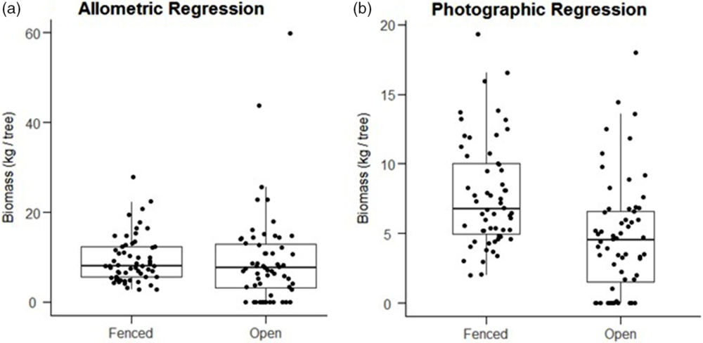
Figure 5. Boxplots showing the distribution of modeled biomasses for individual trees, pooled by fenced plots (n = 58 trees) and open plots (n = 59 trees). Predictions of the Okello allometric equation (a) do not show a significant difference between fenced and open plots (1 sided t-test, P = 0.43). Predictions of the photographic regression (b) do show significantly greater biomass in fenced plots (1-sided t-test, P < 0.001).
Discussion
Our photographic technique accurately predicted above-ground biomass of A. drepanolobium and was a substantial improvement over an existing allometric equation. Using this method, we were able to quantify the significant difference in above-ground biomass between unfenced and herbivore-exclosure plots, attributable to herbivore browsing. This contrast was apparent from a visual survey of the plots and was reflected in significant differences in tree height and diameter. However, the biomass estimates from the existing allometric equation of Okello et al. (Reference Okello, O’Connor and Young2001) did not accurately capture these differences, demonstrating the need for a complementary method to quantify changes in biomass due to herbivory. In addition, we did not find an effect of ant occupant, suggesting that differences in architecture induced by ants do not affect total biomass. Our photographic method provides an important extension to existing methods for quantifying changes in above-ground biomass.
In Laikipia and other regions of Kenya, A. drepanolobium is a key component of several large mammals’ diets, including elephants (Loxodonta africana), reticulated giraffes (Giraffa camelopardalis reticulata) and black rhino (Diceros bicornis) (Birkett Reference Birkett2002, Kartzinel et al. Reference Kartzinel, Chen, Coverdale, Erickson, Kress, Kuzmina, Rubenstein, Wang and Pringle2015). Additionally, A. drepanolobium fixes nitrogen and partially drives nutrient dynamics and forage quality (Fox-Dobbs et al. Reference Fox-Dobbs, Doak, Brody and Palmer2010). Tracking changes in this acacia’s biomass is therefore important for understanding both food availability for browsers and forage quality for all herbivores. This is particularly pertinent because A. drepanolobium in Laikipia County may experience wide-scale changes in abundance and cover due to increasing disturbance from invasive species (Riginos et al. Reference Riginos, Karande, Rubenstein and Palmer2015), charcoal harvesting (Okello et al. Reference Okello, O’Connor and Young2001) and land use change (Muriithi Reference Muriithi2016).
Across most savannas, tree biomass and cover are important drivers of ecosystem structure and function (Holdo et al. Reference Holdo, Holt and Fryxell2009). Trees provide food for browsers, fix nutrients in soil, serve as habitat for arthropods and nesting sites for birds, and modify mammal movement and habitat use. Therefore, accurately measuring tree biomass is not only a desirable goal in itself but will also enhance our understanding of savanna ecology and aid in the management of endangered species. Yet characterizing abundance, biomass and size structure of trees has been a long-standing challenge in savanna ecosystems (Archer Reference Archer, Hodgson and Illius1996, House et al. Reference House, Archer, Breshears and Scholes2003), particularly for remote sensing approaches (Munyati et al. Reference Munyati, Shaker and Phasha2011). While there have been photographic techniques developed to measure vegetative cover or shrub biomass (Louhaichi et al. Reference Louhaichi, Johnson, Woerz, Jasra and Johnson2010, Reference Louhaichi, Hassan, Clifton and Johnson2017), these studies were conducted in arid regions in which low vegetation (forbs and shrubs) stood out starkly against a background of bare earth when viewed from above. In contrast, savannas are characterized by a matrix of grass that can be spectrally confused with the trees of interest (Cho et al. Reference Cho, Mathieu, Asner, Naidoo, van Aardt and Ramoelo2012). Likewise, a similar method (Ter-Mikaelian & Parker Reference Ter-Mikaelian and Parker2000) measured biomass on small, relatively isotropic seedlings that were not structurally altered by herbivory. But larger trees (1–3 m) present more 3-dimensional complexity and may suffer from significant asymmetry due to herbivory; consequently, they need to be photographed from multiple angles at ground level.
Our method is substantially less expensive than LiDAR, costing only a few hundred dollars for a camera, tripod and backdrop. It is ideal for small-scale projects in which it is inexpensive to employ 3–5 personnel to survey trees, although windy conditions can make holding the contrast backdrop physically taxing. However, our method is more laborious than LiDAR, and could not realistically be used to measure trees at scales of tens or hundreds of hectares. In cases where larger scales are of interest, our technique will provide indispensable ground truth measurements by which to calibrate other forms of remote sensing, including LiDAR or aerial biomass estimates (Shepaschenko et al. Reference Schepaschenko, Chave, Phillips, Lewis, Davies, Réjou-Méchain, Sist, Scipal, Perger, Hérault and Labrière2019). In sum, our method provides an accurate, cost-effective and relatively efficient complement to existing methods for detecting changes in above-ground biomass of trees across space or through time.
A major obstacle is the extensive photo processing time required to classify photos of trees manually. If an accurate algorithmic classification scheme could be implemented, it would reduce the time investment considerably. Although our classification of photos was necessarily subjective, it was still considerably more accurate than any of the algorithmic approaches we attempted. Finally, those intending to use this technique should opt for the highest resolution (megapixel) camera available, as this will increase the accuracy of results.
Beyond savannas, accurately and efficiently estimating biomass of small trees should be useful for forest managers quantifying understorey biomass or comparing total biomass of a single species at different life stages (Hubau et al. Reference Hubau, De Mil, Van den Bulcke, Phillips, Ilondea, Van Acker, Sullivan, Nsenga, Toirambe, Couralet and Banin2019). In particular, it will be useful for measuring change in biomass of individual trees over time, allowing for more precise calculation of growth rates under different environmental conditions. A similar photographic technique was used to quantify tree architecture and measure similarity of traits between individuals in a study of herbivore community assembly (Barbour et al. Reference Barbour, Rodriguez-Cabal, Wu, Julkunen-Tiitto, Ritland, Miscampbell, Jules and Crutsinger2015). Any study in which researchers wish to quantify browsing more accurately than commonly used qualitative metrics will also benefit from this method. We hope that this technique will find broad use with anyone seeking to measure above-ground biomass of relatively small (<5 m) trees.
Acknowledgements
We acknowledge the support of the National Science Foundation as well as the collaboration of Ol Pejeta Conservancy and Mpala Research Centre. J. Alston helped with coding, K. Driese reviewed this manuscript, and many helped with fieldwork: G. Busieni, S. Carpenter, J. Eckadeli, J. Gitonga, N. Maiyo, P. Milligan, G. Mizell, J. W. Murage, A. Njenga, A. Pietrek and K. Steinfield.


