Introduction
Savannas are one of the world’s most important biomes. They are characterized by plant communities with co-dominance of scattered woody species and a continuous grass stratum (Belsky Reference Belsky1984, Frost & Robertson Reference Frost, Robertson, Walker and Walker1985, Sankaran et al. Reference Sankaran, Ratnam and Hanan2004, Reference Sankaran, Hanan, Scholes, Ratnam, Augustine and Cade2005). Land use, recurring fires, large herbivores and livestock all influence the diversity and structure of plant communities in tropical savannas. Frequent fires reduce the abundance of herbs and small shrubs, mainly by killing or suppressing seedlings and saplings of fire-sensitive plant species (Frost & Robertson Reference Frost, Robertson, Walker and Walker1985, Morrison et al. Reference Morrison, Cary, Pengelly, Ross, Mullins, Thomas and Anderson1995, Trapnell Reference Trapnell1959). Browsers, especially elephants, cause serious damage to tree and shrub canopies, reduce the growth rate of twigs, and in general, suppress tree and shrub encroachment (Augustine & McNaughton Reference Augustine and McNaughton2004). Indeed, exclosure experiments in savannas have shown that large herbivores increase bare ground area and reduce woody canopy cover (Asner et al. Reference Asner, Levick, Kennedy-Bowdoin, Knapp, Emerson, Jacobson, Colgan and Martin2009, Young et al. Reference Young, Porensky, Riginos, Veblen, Odadi, Kimuyu, Charles and Young2018). In contrast, grazers including livestock reduce the tree–grass competitive balance, resulting in an increase in trees abundance (Kimuyu et al. Reference Kimuyu, Sensenig, Riginos, Veblen and Young2014, Langevelde et al. Reference Langevelde, Van Der Vijver, Kumar, Van Der Koppel, Ridder, Andel, Skidmore, Hearne, Stroosnijder, Bond, Prins and Rietkerk2003, Roques et al. Reference Roques, O’Connor and Watkinson2001).
The role of biotic factors in shaping species diversity and distributions in savannas is fairly well understood. In contrast the effects of abiotic factors have been poorly studied in this biome. At a subcontinental level, it has been determined that tree height, tree cover, basal area and woody species richness all decrease in savannas with decreasing rainfall and increasing soil clay content (Williams et al. Reference Williams, Duff, Bowman and Cook1996). Local variation in topography is widely recognized as one of the most important determinants of vascular plant diversity (Moeslund et al. Reference Moeslund, Arge, Bøcher, Dalgaard and Svenning2013). Topography can temporarily influence the patterns of water loss and accumulation which in turn can shape the patterns of species distribution (Coughenour & Ellis Reference Coughenour and Ellis1993, Wu & Archer Reference Wu and Archer2005). The role of topography in regulating species diversity and distribution has been widely investigated in forest ecosystems (Chuyong et al. Reference Chuyong, Kenfack, Harms, Thomas, Condit and Comita2011, Gunatilleke et al. Reference Gunatilleke, Gunatilleke, Esufali, Harms, Ashton, Burslem and Ashton2006, Harms et al. Reference Harms, Condit, Hubbell and Foster2001, Lai et al. Reference Lai, Mi, Ren and Ma2009), but research is still lacking in savannas.
We established a large (120 ha) long-term monitoring plot to understand the dynamics of tree and shrub populations and explore the physical patterns of biodiversity within a savanna landscape. The plot is located in an Acacia–tall grass savanna in central Kenya that undergoes heavy grazing by livestock and large herbivores, a state common to savannas in this region. The plot is topographically diverse, and traverses two main soil types with a transition zone. Thus, it provides an ideal setting for testing the role of physical features of the landscape on savanna tree species distribution and richness. Here, we present the patterns of tree and shrub (hereafter tree) diversity in the plot and investigate species–topographic habitat associations by testing the following hypotheses: (1) Savanna structure and tree species composition vary with topography; and (2) a large proportion of species are significantly associated to the different topographic habitats.
Methods
Study site
The study was carried out in the Mpala Ranch (Figure 1, hereafter Mpala), 195 km2 of unfenced conservancy located on a large plateau in the northern part of the central highlands of Kenya, north-west of Mt Kenya, and 43 km north-east of the city Nanyuki in the Laikipia district (36°10′–37°3′E, 0°17′S–0°45′N). Between 1999 and 2016 rainfall at Mpala averaged 646 mm y−1, with high precipitation (>1000 mm) in 2012 (Caylor et al. Reference Caylor, Gitonga and Martins2017, Young et al. Reference Young, Okello, Kinyua and Palmer1997). Warm days and cool nights predominate, with very low humidity in the driest season (January–April), and moderate humidity at other times. Temperatures range between 12°C and 24°C. Anthropogenic fires in the ranch stopped during the 1960s and only sporadic accidental low-scale fires have been recorded in recent years (Kimuyu et al. Reference Kimuyu, Sensenig, Riginos, Veblen and Young2014).
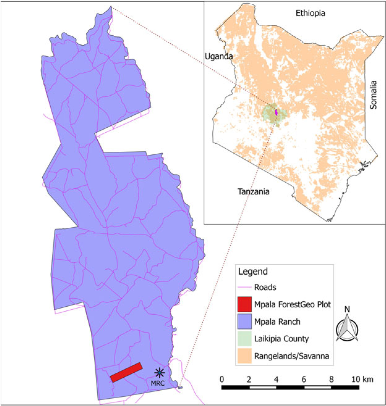
Figure 1. Location of the Mpala plot in Mpala Ranch, Central Kenya.
The vegetation of the area is classified as Acacia–tall grass savanna dominated by Acacia species (Edwards Reference Edwards1940). An estimated 600–800 plant species, 300 species of birds and at least 70 mammal species including impala, zebra, scrub hare, waterbuck, Cape buffalo, eland, Günther’s dik-dik, rodents and elephant, as well as predators such as spotted hyena, lion, leopard and wild dog, are found within the Mpala conservancy (Young et al. Reference Young, Okello, Kinyua and Palmer1997).
Plot establishment
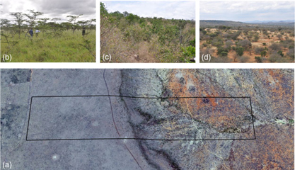
The Mpala plot is 120 ha (2400 × 500 m), with the long axis oriented SW–NE. The geographic coordinates of the south-west corner are 0°17′30.48′′N, 36°52′51.24′′E and the altitude ranges from 1668–1792 m asl. The plot consists of an almost flat plateau in the south-west and descends through steep slopes to a lower area in the north-east, with undulating topography (Figure 2a). The plot traverses the two major soil types of the Laikipia area. The first 50 ha towards the south-west end of the plot (at higher altitude) lie on poorly drained deep clay nutrient-rich vertisols, also known as black-cotton soils, which changes gradually (about 15 ha) to the red rocky friable sandy loams at the lower end of the plot (lower altitude). The plot lacks any permanent stream (Figure 2a). However, there are a few marshy areas in the lower end of the plot, and a small creek with temporary streams.

Figure 2. Variation of soil and vegetation types in the 120-ha plot in Mpala, Kenya. Aerial photograph showing the location of the plot and the two main soil types (a). Vegetation of the black cotton soil (b). Vegetation of the cliff on transition soils (c). Vegetation of the lowest part of the plot on the red soils (d).
The establishment of the plot was initiated in 2010, following standard methods (Condit Reference Condit1998) of the Forest Global Earth Observatory (ForestGEO, https://forestgeo.si.edu/). The plot was surveyed and permanently demarcated in the horizontal plane into 3000 quadrats of 400 m2 (20 × 20 m) each and the altitude was then measured at each corner post. Because of the short stature and low branching of the majority of the trees and the abundance of shrubs in the plot, the diameter of trees was measured at 0.5 m (instead of 1.3 m) above ground level (diameter at knee height, dkh). In 66 ha, all free-standing trees with dkh ≥1 cm were tagged, mapped, measured and identified to species/morphospecies. In the remaining 54 ha, only trees with dkh ≥2 cm were included in the census. For plot-wide analyses presented in this paper, we use only data with dkh ≥2 cm. Tree species identification was done in the field and in the herbarium. Vouchers from all morphospecies are housed at the East African Herbarium (EA) at National Museums of Kenya, Nairobi and the Smithsonian herbarium (USA). Species’ nomenclature follows Beentje et al. (Reference Beentje, Adamson and Bhanderi1994). In spite of recent proposals to split the genus Acacia into Vachellia and Senegalia (Kyalangalilwa et al. Reference Kyalangalilwa, Boatwright, Daru, Maurin and Van Der Bank2013), we follow a more conservative, inclusive definition of the genus Acacia. All plot data are managed following ForestGEO standards (Condit et al. Reference Condit, Lao, Singh, Esufali and Dolins2014).
Topography and habitat categorization
Habitats within the Mpala plot were defined by three physical parameters, i.e. altitude, slope and convexity, calculated in a regular 5 × 5-m grid, and then assigned to 20 × 20-m quadrats that divided the plot. For each quadrat, the altitude was calculated by averaging the altitude of the four corners. The slope of the quadrat was obtained by dividing the quadrat into four triangular planes, each consisting of three joined corners of the quadrat, and then averaging the angular deviation of the four planes from the horizontal. Convexity was calculated by substracting the mean altitude of the focal quadrat from the mean altitude of the eight surrounding quadrats. For edge quadrats, convexity was obtained by substracting the altitude of their centre point from the mean altitude of their four corners (Yamakura et al. Reference Yamakura, Kanzaki, Itoh, Ohkubo, Ogino, Chai, Lee and Ashton1995). Negative values of convexity denoted concave quadrats while positive values indicated convex quadrats. After standardization, the three variables were used to group the 3000 quadrats of the plot into four groups (habitats) using the Ward hierarchical clustering (Ward Reference Ward1963). The four habitats were the plateau which largely overlaps with the black-cotton soils; the cliff, mostly on transition soils; the low plain; and the depressions that overlap with the red soils (Figure 3). The means, the minima and the maxima of the three topographic variables for each habitat are provided in Table 1.

Figure 3. Topographic map of the Mpala 120-ha (2400 × 500 m) plot with 10-m contour interval and overlay of the four topographic habitats defined in the study, based on altitude, slope and convexity.
Table 1. Area, mean and range of the three physical parameters characterizing the four topographic habitats delimited within the Mpala plot

Floristic and structural parameter calculations and species habitat test
To characterize the tree community within the plot, the number of species, the Fisher’s alpha, the basal area and tree abundances were calculated by averaging the values in 120 subplots of 1 ha (100 × 100 m) each within the plot. To assess the structural and floristic differences among the four topographic habitats, the same parameters were calculated for 20 × 20-m quadrats.
Species–habitat associations
Species–habitat associations were determined for the 30 most abundant species (≥1 individual ha−1), using the torus-translation test (Harms et al. Reference Harms, Condit, Hubbell and Foster2001). The test evaluates if significant associations are present between the spatial distribution of a focal species and a given habitat. This is achieved by translating the habitat map in four cardinal directions, moving the entire habitat map one column or row of 20 × 20-m quadrats at a time, resulting in 2999 translations for the plot. The observed relative densities of individuals in each of the habitats is compared with the expected relative densities. With an approximated P-value of ∼0.05, a relative density in the true habitat map >97.5% of the values obtained from translated maps denoted a positive association. Significant negative associations were those with the relative density in the true map <97.5% of the values obtained from the translated maps. The analysis was performed in R (https://cran.r-project.org), using the function tt_test of the package fgeo.habitat (https://github.com/forestgeo/fgeo.habitat).
Results
Stand structure and floristics
A total of 245 578 stems belonging to 113 337 individuals with dkh ≥2 cm were inventoried in the plot. These individuals included 63 morphospecies,41 genera and 22 families (Appendix 1, Table 2). Ninety-eight per cent of all individuals (52 morphospecies) were identified to species level, 2% of the individuals (11 morphospecies) were identified to genus level, and 28 individuals were not identified because they were leafless during the enumeration and died before we could collect good voucher specimens. The Fabaceae with 12 species in three genera were the richest family in the plot, followed by the Malvaceae and Rubiaceae (Table 3). The genera Acacia and Grewia were the most species-rich in the plot, with 10 and 6 species respectively (Table 3). For all trees with dkh ≥2 cm, there were 18 species ha−1, but only five species ha−1 for all trees with dkh ≥10 cm and two species ha−1 and two for larger trees with dkh ≥30 cm. For the entire plot, Fisher’s alpha was 6.56 for trees with dkh ≥2cm and 4.86 for trees with dkh ≥10 cm (Table 2).
Table 2. Summary of the floristics of the Mpala 120-ha plot: Number of individuals, basal area (m2), number of tree species, of genera and families, and Fisher’s alpha the entire 120 ha and per ha. The means are calculated by averaging the values in 120 subplots of 100 × 100-m each. dkh (diameter at knee height) is the diameter of trees measured at 0.5 m above ground

Table 3. Five most important families in terms of abundance, basal area and number of species for trees with dkh ≥ 2 cm in the 120-ha Mpala plot. BA = basal area in m2 ha−1

Abundance and basal area
For all individuals with dkh ≥2 cm, tree density was 944 individuals ha−1 and only 66 individuals ha−1 for trees ≥10 cm. Basal area was 3.71 m2 ha−1 for all trees ≥2 cm, and 1.29 m2 ha−1 for larger trees with dkh ≥10 cm. The Fabaceae with 513 individuals ha−1 were the most abundant family, followed by Ebenaceae and Euphorbiaceae. The Fabaceae also had the highest basal area (2.44 m2 ha−1), followed again by the Ebenaceae and Euphorbiaceae (Table 3).
The genus Acacia (Fabaceae) was the most abundant, representing 54% of all individuals in the plot. Euclea (Ebenaceae) was the second most abundant genus, representing 17% of all individuals. The genera with the highest basal area were Acacia and Euclea (Table 4). Acacia drepanolobium had the highest density, with 212 individuals ha−1, accounting for 22% of the total individuals with dkh ≥2 cm. Euclea divinorum followed with 165 individuals (17% of the total). Acacia brevispica and Croton dichogamus accounted for 16% each. The remaining species accounted for <10% of the total individuals (Table 5). Thirty-three species (51% of the total) were rare, with <1 individual ha−1. The five most important species in terms of basal area were Acacia mellifera, A. etbaica, Euclea dinovirum, A. drepanolobium and A. gerrardii (Appendix 1).
Table 4. Five most important genera in terms of abundance, basal area and number of species for trees with dkh ≥2 cm in the 120-ha Mpala plot. BA = basal area in m2 ha−1

Table 5. The 10 most abundant tree species in Mpala plot with their densities in the entire plot and different topographic habitats. Numbers in parentheses indicate the rank in abundance of the species in the plot or the habitat

Stand structure and floristic variation among habitats
The plateau habitat on clay soils had the lowest tree density, the lowest basal area, the lowest species richness and the lowest Fisher’s alpha. Tree density, species richness and Fisher’s alpha were highest on the cliff. This habitat had the highest tree density especially of small-sized diameter (dkh 2–4 cm), but also the second lowest basal area due to the low proportion of large trees (dkh >15 cm). The bigger trees in the plot are concentrated in the lower end of the plot that also has the highest basal area (Table 6, Figure 2b).
Table 6. Tree density, basal area, species richness and Fisher’s alpha of the topographic habitats in the 120-ha Mpala plot. The habitat-wide values are calculated per ha (100 × 100 m) and the quadrat values are for 20 × 20-m quadrats

All dominant species had consistently low densities in the plateau habitat, except for Acacia drepanolobium, which dominates this habitat with 487 individuals ha−1 (550 for all trees with dkh ≥2 cm) and making 94% of all trees with dkh ≥2 cm. The densities of the other dominant species were inconsistent across the remaining habitats. The density of Croton dichogamus in the cliff (552 individuals ha−1) was more than five times higher than in the low plain and depression habitats respectively. Despite having different densities, dominant species have nearly similar ranks in the low plain and depressions habitats (Table 5).
Species–habitat association
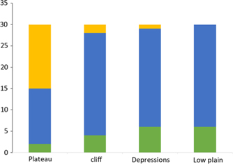
Of the 30 species subjected to the species–habitat association test, 21 (70%) were either negatively or positively associated to one or two of the four topographic habitats. The remaining nine species were neutral (that is, not significantly associated with any of the habitats) (Figure 4, Appendix 2). Fifteen species were positively associated to one habitat. The distribution maps of selected species positively associated to each habitat are presented in Figure 5. The low plain and the depressions had the highest number of positive associations (five species each) and the plateau had the lowest (two species). No species was positively associated to more than one habitat. Half of the species were negatively associated to the plateau while no species was negatively associated to the low plain habitat. Acacia drepanolobium was the only species negatively associated to more than one habitat.

Figure 4. Species–habitat associations of 30 species of trees with dkh ≥2 cm and ≥120 individuals in the Mpala plot, based on a two-tailed torus-translation test. Three types of association are indicated: significant positive association (green), neutral association (blue) and significant negative association (orange).
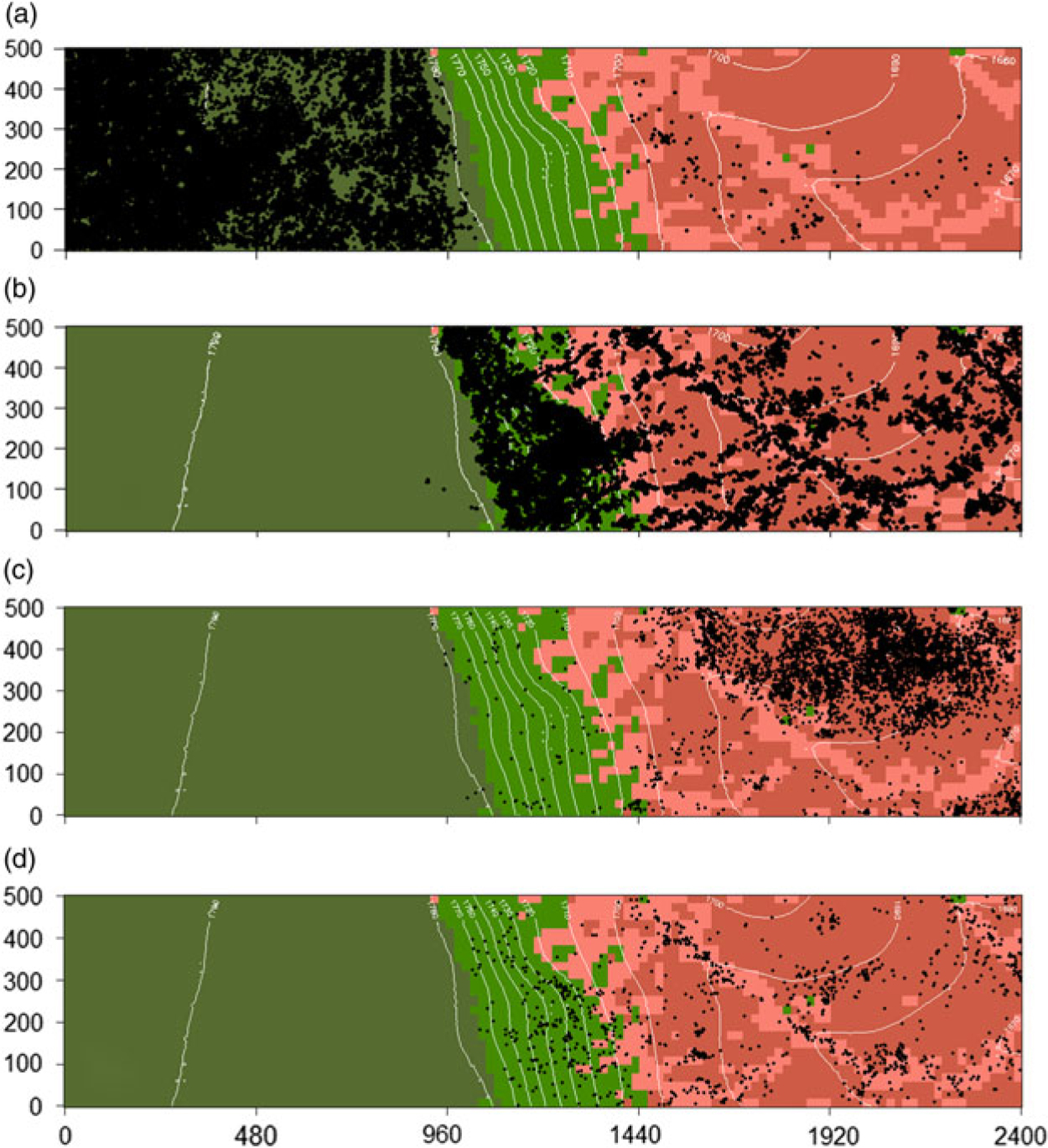
Figure 5. Distribution maps of selected species positively associated to the four topographic habitats in the 120-ha (2400 × 500 m) Mpala plot. Plateau – Acacia drepanolobium (a), cliff – Croton dichogamus (b), low plain – Acacia etbaica (c), depressions – Grewia lilacina (d).
All the species positively associated to one habitat were also negatively associated to the plateau habitat, except for Acacia drepanolobium, A. mellifera and A. gerardii (Appendix 2). Seventeen species (57%) were negatively associated to one or two habitats, of which 15 were negatively associated to the plateau. Phyllanthus sepialis, known to grow in riverine formations (Beentje et al. Reference Beentje, Adamson and Bhanderi1994), was negatively associated to the plateau habitat, but surprisingly not associated to the depressions (Appendix 2).
Discussion
Structure and diversity
We inventoried 63 species of trees with dkh ≥2 cm within 1.2 km2 of non-protected savanna in Central Kenya. As expected, the species richness (18 species ha−1) was low compared with other tropical biomes with comparable data (Anderson-Teixeira et al. Reference Anderson-Teixeira, Davies, Bennett, Gonzalez-Akre, Muller-Landau and Joseph Wright2015). Species richness varied by five to seven orders of magnitude across the topographic gradient, with the south-west end of the plot on clay soils having the lowest number of species. The variation in topography in the plot almost overlaps with the variation in soil types, both of which could explain the change in species composition across the plot. Such a change has already been reported in the savanna biome, though at a smaller scale. Moe et al. (Reference Moe, Mobæk and Narmo2009) showed a turnover in species between termite mounds and the adjacent Acacia savanna in Uganda. Similarly, Cox & Gakahu (Reference Cox and Gakahu1985) showed differences in grass and tree species composition between Mima mounds and the surrounding savanna on black cotton soil in Central Kenya. However, the impact of both livestock and large herbivores could have contributed to the low tree species diversity of the plot (Georgiadis et al. Reference Georgiadis, Olwero, Ojwang’ and Romañach2007, Kinnaird & O’Brien Reference Kinnaird and O’Brien2012). Augustine & McNaughton (Reference Augustine and McNaughton2004) showed in the Mpala Ranch that the combined effect of browsers of different sizes, from dik-dik to elephant, results in a significant reduction of leaf density, leaf biomass and growth rate of twigs, tree cover and seedling recruitment, thus reducing tree establishment. Elsewhere, high densities of elephants have been shown to significantly alter the structure and composition of savannas (Cumming et al. Reference Cumming, Fenton, Rautenbach, Taylor, Cumming, Cumming, Dunlop, Ford, Hovorka and Johnston1997). Tree density was three and two times higher on the cliff, low plain and depressions habitats respectively, than on the plateau habitat. The low tree density observed in this area of the plot can be attributed to the soil type, but also to the suppressing effect of large herbivores. Indeed, experimentally excluding elephants and other large mammals (Young et al. Reference Young, Okello, Kinyua and Palmer1997) in a similar habitat increased tree density by 42% (Kimuyu et al. Reference Kimuyu, Sensenig, Riginos, Veblen and Young2014).
The Mpala plot is dominated by Fabaceae among which Acacia drepanolobium alone represents 22% of all individuals in the plot. The success of this species lies on its singular ability to adapt to harsh edaphic conditions of the black-cotton soil (Pringle et al. Reference Pringle, Prior, Palmer, Young and Goheen2016) and the mutualistic relation with associated ants that significantly reduce herbivory (Goheen & Palmer Reference Goheen and Palmer2010, Madden & Young Reference Madden and Young1992, Palmer et al. Reference Palmer, Doak, Stanton, Bronstein, Kiers, Young, Goheen and Pringle2010).
Species–habitat associations and their maintenance
Several studies have shown the importance of microtopographic habitats as drivers of plant species distribution in large census plots, especially in tropical rain forests (Chuyong et al. Reference Chuyong, Kenfack, Harms, Thomas, Condit and Comita2011, Gunatilleke et al. Reference Gunatilleke, Gunatilleke, Esufali, Harms, Ashton, Burslem and Ashton2006, Harms et al. Reference Harms, Condit, Hubbell and Foster2001, Lai et al. Reference Lai, Mi, Ren and Ma2009, Pei et al. Reference Pei, Lian, Erickson, Swenson, Kress, Ye and Ge2011, Valencia et al. Reference Valencia, Foster, Villa, Condit, Svenning, Hernández, Romoleroux, Losos, Magård and Balslev2004). Our study is the first of its kind in a savanna biome. We show that as in tropical rain forest, microtopographic habitats can play an essential role in shaping the structure of the vegetation and tree species distribution in savannas. Thirty-six per cent of the species were positively associated to one of the topographic habitats. In the Mpala plot, this species-habitat association indirectly supports the idea of soil-nutrient niche partitioning (Andersen et al. Reference Andersen, Turner and Dalling2010, Paoli et al. Reference Paoli, Curran and Zak2006, Russo et al. Reference Russo, Davies, King and Tan2005), given the variation in soil of the defined topographic habitats.
Two-thirds of the species were negatively associated to the plateau habitat, suggesting that this habitat is stressful for tree species establishment. In fact, the black-cotton soils that prevail in this habitat undergo shrink-swell and cracking cycles, with limited water infiltration and low water potentials during the dry season (Pringle et al. Reference Pringle, Prior, Palmer, Young and Goheen2016). These conditions are physically challenging for seedling establishment and contribute to the maintenance of low species diversity in this habitat. The cliff habitat was dominated by small shrubs, had the highest tree abundance, fewer large trees and therefore the lowest basal area (Table 6). This pattern could be explained by the shallow soils and drier conditions imposed by the high slope that does not allow high water infiltration after rain (Coughenour & Ellis Reference Coughenour and Ellis1993). In the low-altitude habitats, the nutrient-poor sandy loams provide less stressful conditions and have more positively associated species.
Less than half of the species showed positive associations to the defined topographic habitats in the Mpala plot. In contrast, a higher proportion of species (70%) showed significant negative associations. These results indicate that the low tree species richness in the plot cannot be explained by the lack of topographic niche partitioning in this savanna. Soil texture and nutrients seem to have a stronger effect on species distributions. The sharp difference in plant community composition between the black-cotton and the red soils is also maintained by large-mammal herbivory. Evidence from field experiments showed that in the absence of large herbivores, transplanted seedlings of A. drepanolobium (monodominant on black cotton soil) and A. brevispica (dominant on sandy loams) establish on both soil types (Pringle et al. Reference Pringle, Prior, Palmer, Young and Goheen2016). However, browsers suppress the growth and survival of A. drepanolobium on sandy soils, while the combination of elephant browsing and stress from the cracking clay vertisols prevents most A. brevispica from attaining maturity on black-cotton soils (Pringle et al. Reference Pringle, Prior, Palmer, Young and Goheen2016). This means that biotic processes can mediate the habitat–species associations observed within the plot and attributed to purely environmental (abiotic) conditions.
As reported in tropical forests, topographic variation is an important factor that contributes in shaping local tree species diversity, distribution and composition in African savannas. In the specific case of Mpala Ranch, habitat specificity is maintained by the interaction between large-mammal herbivory and the edaphic variation among the topographic habitats.
Author ORCIDs
David Kenfack https://orcid.org/0000-0001-8208-3388
Acknowledgements
Special thanks go to the Mpala plot field leaders Staline Kibet, David Melly, Kimani Ndung’u, Solomon Kipkoech, Augustine Chebos, Barnabas Bolo and S. Akwam who were instrumental in running the first census and supervising the field crews. The field assistants Gilbert Busienei, Abdi Aziz Hassan, Sammy Ethekon, George Koech, Robert Malakwen, Peter Lorewa, Julius Nairobi, Nicholas Kipsuny, Buas Kimiti, David Sangili and Eripon Samson Eloiloi are also acknowledged for their effort and hard work in the field during the first census and thereafter. Also, we are grateful to the National Museums of Kenya and the Mpala Research Centre, especially to Dino Martin, Margaret Kinnaird, Gikenye Chege, Tuni Bara for the administrative and infrastructural help. Finally, we appreciate Ms Suzanne Lao for help with data management and screening, Drs Stuart Davies, Sean McMahon and Gabriel Arellano for their constructive critique on the early manuscripts of this paper. The location map was drawn by Duncan Kimuyu.
Financial support
The 120-ha Mpala plot is a collaborative project of the National Museums of Kenya and the Mpala Research Centre in partnership with the Forest Global Earth Observatory (ForestGEO) of the Smithsonian Tropical Research Institute (STRI). Funding for the first census was provided by ForestGEO.
Appendix 1
Total number of individuals and total basal area (m2) for each of the 63 species of trees with dkh ≥2 cm recorded in the Mpala 120-ha plot

Appendix 2
Species–habitat association randomization test result of the 30 most abundant species in the Mpala plot. N = number of individuals, Sig = significance of the test: 1 = positive association, −1 = negative association, 0 = neutral