


INTRODUCTION
Marine coastal ecosystems include intertidal and nearshore systems that are influenced by atmospheric, terrestrial and autochthonous processes (Kennedy et al., Reference Kennedy, Twilley, Kleypas, Cowan and Hare2002; Carr et al., Reference Carr, Neigel, Estes, Andelman, Warner and Largier2003; Ruttenberg & Granek, Reference Ruttenberg and Granek2011; Bahloul et al., Reference Bahloul, Chabbi, Dammak, Amdouni, Medhioub and Azri2015). These ecosystems are generally sensitive to changes in upstream terrestrial systems and to direct inputs (Ruttenberg & Granek, Reference Ruttenberg and Granek2011). Thus, they are undergoing significant and growing anthropogenic threats (Cloern, Reference Cloern2001; Newton et al., Reference Newton, Icely, Falcao, Nobre, Nunes, Ferreira and Vale2003; Beaugrand et al., Reference Beaugrand, Edwards and Legendre2010; Brander, Reference Brander2010; Burrows et al., Reference Burrows, Schoeman, Buckley, Moore, Poloczanska, Brander, Brown, Bruno, Duarte, Halpern, Holding, Kappel, Kiessling, O'Connor, Pandolfi, Parmesan, Schwing, Sydeman and Richardson2011; Bahri-Trabelsi et al., Reference Bahri-Trabelsi, Armi, Trabelsi-Annabi, Shili and Ben Maiz2013; Bahloul et al., Reference Bahloul, Chabbi, Dammak, Amdouni, Medhioub and Azri2015; Serranito et al., Reference Serranito, Aubert, Stemmann, Rossi and Jamet2016).
Zooplankton plays a pivotal role in aquatic food webs by transferring carbon to higher trophic levels, consuming microorganisms (bacteria, protists) and serving as a prey for fish and invertebrates (De-Young et al., Reference De-Young, Heath, Werner, Megrey and Monfray2004; Sampey et al., Reference Sampey, Mckinnon, Meekan and McCormick2007; Ziadi et al., Reference Ziadi, Dhib, Turki and Aleya2015). Zooplankton communities are known to quickly respond to fluctuations in environmental factors particularly in coastal areas where the combination of land and marine influences drives strong spatiotemporal variability (Siokou-Frangou, Reference Siokou-Frangou1996). Zooplankton can thus be considered as useful indicators of ecosystem health status (Hays et al., Reference Hays, Richardson and Robinson2005; Longhurst, Reference Longhurst2007). The presence or absence of certain zooplankton species may indicate the relative influence of different water types on ecosystem structures and may serve as an early indication of a biological response to environmental and climatic changes (Hays et al., Reference Hays, Richardson and Robinson2005; Ziadi et al., Reference Ziadi, Dhib, Turki and Aleya2015). Zooplankton signatures may characterize specific hydrographic conditions in most of the world's ecosystems. Several studies have been undertaken in the Gulf of Gabes regarding the characterization of local zooplankton assemblages (Drira et al., Reference Drira, Bel Hassen, Ayadi, Hamza, Zarrad, Bouaïn and Aleya2010a, Reference Drira, Hamza, Bel Hassen, Ayadi, Bouaïn and Aleyab, Reference Drira, Bel Hassen, Ayadi and Aleya2014; Ben Ltaief et al., Reference Ben Ltaief, Drira, Hannachi, Bel Hassen, Hamza, Pagano and Ayadi2015, Reference Ben Ltaief, Drira, Devenon, Hamza, Ayadia and Pagano2017). In this area, the functioning of the coastal environments is highly complex due to the interaction of various factors, i.e. water movements, tide currents, anthropogenic inputs, marine traffic and fishing activities (Drira et al., Reference Drira, Hamza, Bel Hassen, Ayadi, Bouaïn and Aleya2008, Reference Drira, Kmiha-Megdiche, Sahnoun, Hammami, Allouche, Tedetti and Ayadi2016; Feki et al., Reference Feki, Hamza, Frossard, Abdennadher, Hannachi, Jacquot, Bel Hassen and Aleya2013). The Gulf of Gabes is subject to a variety of human activities (Bejaoui et al., Reference Bejaoui, Raïs and Koutitonsky2004; Gargouri et al., Reference Gargouri, Azri, Serbaji, Jedoui and Montacer2011, Reference Gargouri, Bahloul and Chafai2015). These activities include urban settlements, industrial areas and intense maritime traffic, resulting in the discharge of industrial and municipal effluents enriched in nutrients and pollutants which might negatively affect the water quality and the state of the ecosystem (Bejaoui et al., Reference Bejaoui, Raïs and Koutitonsky2004; Gargouri-Ben Ayed et al., Reference Gargouri-Ben Ayed, Souissi, Soussi, Abdeljaouad and Zouari2007; Gargouri et al., Reference Gargouri, Azri, Serbaji, Jedoui and Montacer2011, Reference Gargouri, Bahloul and Chafai2015; Aloulou et al., Reference Aloulou, Elleuch and Kallel2012; Ben Salem et al., Reference Ben Salem, Drira and Ayadi2015; Ben Salem & Ayadi, Reference Ben Salem and Ayadi2016; Drira et al., Reference Drira, Kmiha-Megdiche, Sahnoun, Hammami, Allouche, Tedetti and Ayadi2016, Reference Drira, Sahnoun and Ayadi2017).
The main goal of this study was to improve knowledge about the spatial distribution of zooplankton abundance and composition in a large spectrum of three coastal areas in the Gulf of Gabes characterized by different degrees of pollution: (1) the northern coast of Sfax city which is an area restored via the Taparura project (Callaert et al., Reference Callaert, Van Den Bogaert, Pieters, Pynaert, Tison, Levrau, Vander Heyde and Glaser2009); (2) the southern coast of Sfax city; and (3) Ghannouch coast, close to Gabes city, which is considered as highly polluted. The second aim was to relate the differences observed between the three sampled areas in respect of zooplankton abundance with physical (temperature, salinity and pH), chemical (ammonium ions (NH4+), nitrates (NO3−), nitrites (NO2−), total nitrogen (T-N), orthophosphate (PO43−), total phosphorus (T-P) and silicon atoms ions Si(OH)4) and biogeochemical (suspended particulate matter (SPM), particulate organic carbon and nitrogen (POC and PON), chlorophyll-a (chl-a) and phaeopigment-a (Phaeo-a)) water parameters characterizing the trophic and pollution status of each zone.
MATERIALS AND METHODS
Study area
The Gulf of Gabes (Eastern Mediterranean Sea, between 35°N and 33°N, Tunisia), is endowed with rich aquatic resources contributing to about 65% of the national fish production in Tunisia (DGPA, 2004). Sampling was carried out in the Gulf of Gabes during October and November 2014, in three coastal areas i.e. the southern and the northern coasts of Sfax and the Ghannouch area. Thirty stations were sampled in the Gulf of Gabes among which 10 sampling stations were chosen for each area (SC, NC and GA) taking into account the pollution gradient (Figure 1).

Fig. 1. Location of the studied stations in the southern (stations 1–10) and northern (stations 11–20) coastal areas of Sfax and the Ghannouch area (stations 21–30) sampled during autumn (October–November 2014).
The coastline of Sfax concentrates a great number of industrial activities, mainly related to phosphates, salt works, tanneries, lead foundry, textiles, ceramics industry, soap factories and building materials (Barhoumi et al., Reference Barhoumi, Messaoudi, Deli, Saïd and Kerkeni2009).
The southern coast of Sfax (hereafter called SC) lies between the fishing harbour in the north and Gargour village in the south. This area is marked by the presence of the Société Industrielle d'Acide Phosphorique et d'Engrais (SIAPE) industry, which has released large amounts of phosphogypsum wastes for 40 years. These phosphogypsum wastes are a significant source of phosphates (PO43−), chloride (Cl−) and sulphates (SO42−) for seawater and may explain the high chemical oxygen demand (COD) in the SC surface waters (Bahloul et al., Reference Bahloul, Chabbi, Dammak, Amdouni, Medhioub and Azri2015; Drira et al., Reference Drira, Kmiha-Megdiche, Sahnoun, Hammami, Allouche, Tedetti and Ayadi2016). Besides the SIAPE industry and its phosphogypsum wastes, the SC comprises several industrial areas related to textiles, tanneries, salt, olive oil, food processing, construction materials, ceramics and glass. Hence, several industrial effluents are released to the sea in this area. All these anthropogenic inputs have been shown to alter the marine environment and biodiversity in SC (Zaghden et al., Reference Zaghden, Kallel, Louati, Elleuch, Oudot and Saliot2005; Gargouri, Reference Gargouri2006; Aloulou et al., Reference Aloulou, Elleuch and Kallel2012; Rekik et al., Reference Rekik, Maalej, Ayadi and Aleya2013; Bahloul et al., Reference Bahloul, Chabbi, Dammak, Amdouni, Medhioub and Azri2015).
The northern coast of Sfax (hereafter called NC), extending from the commercial harbour to wadi Ezzit and beyond, also suffers from the pressure of human activities (Hamza-Chaffai et al., Reference Hamza-Chaffai, Amiard-Triquet and El Abed1997; Tayibi et al., Reference Tayibi, Choura, López, Alguacil and López-Delgado2009) and is subjected to increasing eutrophication with both red (Louati et al., Reference Louati, Elleuch, Kallel, Saliot, Dagaut and Oudot2001) and green tides caused by coastal Ulva rigida replacing the Posidonia oceanica seagrass beds (Ben Brahim et al., Reference Ben Brahim, Hamza, Hannachi, Rebai, Jarboui, Bouain and Aleya2010). Previous studies in NC have focused on the sources and distribution of hydrocarbons in sediments (Louati et al., Reference Louati, Elleuch, Kallel, Saliot, Dagaut and Oudot2001; Zaghden et al., Reference Zaghden, Kallel, Louati, Elleuch, Oudot and Saliot2005) and marine bivalves (Hamza-Chaffai et al., Reference Hamza-Chaffai, Pellerin and Amiard2003).
This area was recently restored through the Taparura project (2006–present), which aimed at remediating this part of Sfax city's coast. The project included the rehabilitation of a former complex industrial site, the reclamation of beaches and restoration of the area (Callaert et al., Reference Callaert, Van Den Bogaert, Pieters, Pynaert, Tison, Levrau, Vander Heyde and Glaser2009). It led to significant improvement of plankton communities and water quality (Rekik et al., Reference Rekik, Maalej, Ayadi and Aleya2013, Reference Rekik, Denis, Maalej and Ayadi2015). Indeed, this zone was strongly polluted by the phosphogypsum wastes from the NPK phosphoric acid industry, situated near the commercial harbour. The NPK was closed in 1992 and the Taparura project allowed the burial and confinement of the phosphogypsum wastes and the rehabilitation of the area between the commercial harbour and Sidi Mansour. In the NC, there are also the outlet of the rainwater drainage channel (‘PK4’), which crosses the city from south-west to north-east, the outlet of the wadi Ezzit, which receives untreated domestic and industrial effluents.
Ghannouch area (hereafter called GA) includes a chemical industry complex as well as a commercial harbour, located 3 km north of Gabes city (Bejaoui et al., Reference Bejaoui, Raïs and Koutitonsky2004). This complex houses the ‘GCT-Gabes’ phosphoric acid industry. Contrary to the SIAPE which stores its phosphogypsum wastes on land in an unprotected dome, the GCT-Gabes directly discharges its phosphogypsum wastes into the sea via an open channel. Organic pollution and drastic pollution by phosphate coming from the discharged sewage waters of the chemical plants of Ghannouch (Zaouali, Reference Zaouali1993) favoured the emergence of green tides and Valonia to Ulva and the red tide or phytoplankton bloom (Hamza-Chaffai et al., Reference Hamza-Chaffai, Cosson, Amiard-Triquet and El Abed1995). This pollution also caused the disappearance of Caulerpa meadows, regression of Posidonia seagrass beds and decreasing diversity of the benthic fauna (Zaouali, Reference Zaouali1993). Besides chemical industries, trawling practices (shrimps fishing) contribute to the deterioration of the Gabes ecosystem as well (Zaouali, Reference Zaouali1993).
Sampling and on board measurements
Sampling was performed on board the vessel ‘Taparura’ between 10:30 am and 3:30 pm (18 and 23 October 2014; SC and NC, respectively), 8:30 am and 12:30 am (13 November 2014; GA) around high tide and under conditions of calm sea and sunny weather. Seawater samples were collected at ~0.1 m depth using 4 l Nalgene® polycarbonate bottles. The bottles were opened below the water surface to avoid sampling of the surface microlayer. They were extensively washed with 1 M hydrochloric acid (HCl) and Milli-Q water before use, rinsed three times with the respective sample before filling and placed in the cold and in the dark after collection.
Zooplankton was collected using a cylindro-conical net (30 cm aperture, 100 cm height, 100 µm mesh size) equipped with an Hydro-Bios flowmeter. The net was towed obliquely from near bottom to surface at each station at a mean speed of 1 m s−1 during 4 mins. After collection, zooplankton samples (200 ml) were rapidly preserved in a buffered formaldehyde solution (2%). They were stained with Rose Bengal to identify the internal tissues of the different zooplankton species and also to facilitate copepod dissection. In situ measurements of temperature, salinity and pH were carried out with measuring cells type TetraCon® 4-electrode system and a refractometer.
Filtration, chemical and biogeochemical analyses and zooplankton identification
Back in the laboratory, samples were immediately filtered under a low vacuum (<50 mm Hg) through pre-combusted (500°C, 4 h) GF/F (~0.7 µm) glass fibre filters (25 or 47 mm diameter, Whatman) using glassware filtration systems. Nutrients, i.e. NO2−, NO3−, NH4+, PO43−, Si(OH)4, T-N and T-P, were analysed with a BRAN and LUEBBE type 3 autoanalyser and their concentrations were determined colorimetrically using a UV-visible 6400/6405 spectrophotometer according to the ‘Standard Methods for the Examination of Water and Wastewater’ (APHA, 1992).
For Chl-a and Phaeo-a analyses, 250–300 ml of samples were filtered. Filters were then extracted with methanol (RP prolabo) according to Raimbault et al. (Reference Raimbault, Lantoine and Neveux2004). After 30 min of extraction in the dark at 4°C, a fluorescence measurement was performed with a fluorometer model 10 Turner Designs (Sunnyvale, USA) at λ Ex/λ Em of 450/660 nm. The acidification method was applied to determine Phaeo-a concentrations. The fluorometer was calibrated with solutions of methanol (96%) and Chl-a (Sigma C5753). For SPM, POC and PON between 250 and 1100 ml of sample were filtered with pre-weighted GF/F filters (the same filter was used for SPM, POC and PON analyses). After filtration, filters were dried at 60°C for 24 h and reweighed on the same balance. SPM concentration was calculated as the difference between filter weight before and after sample filtration, normalized to the filtration volume (Neukermans et al., Reference Neukermans, Ruddick, Loisel and Roose2012). POC and PON quantification were performed simultaneously with an autoanalyser II Technicon (New York, USA), using the wet-oxidation procedure according to Raimbault et al. (Reference Raimbault, Diaz, Pouvesle and Boudjellal1999). POC and PON had a detection limit of 0.50 and 0.10 µm, respectively.
Zooplankton samples were identified according to Rose (Reference Rose1933), Bradford-Grieve (Reference Bradford-Grieve1999) and Costanzo et al. (Reference Costanzo, Campolmi and Zagani2007). The different copepod species were sorted into four demographic classes (nauplii, copepodids, adult males and adult females). Miscellaneous zooplankton were also counted according to Tregouboff & Rose (Reference Tregouboff and Rose1978a, Reference Tregouboff and Roseb). Enumeration was performed under a vertically mounted deep-focus dissecting microscope (Olympus TL 2) and numerical density was expressed in individual m−3. Total length of body size for the adult copepod was measured for each species in each sampled station (10 individuals for each species in each sampling set).
Data processing and statistical analysis
We applied the Geographic Information Systems (GIS) tools using ArcGIS 10.2 version software to make contour plots. Kriging was the method used to build maps relative to spatial distribution for all dataset parameters. Mesozooplankton diversity was measured using a range of univariate and multivariate diversity measurements. Species diversities were assessed using the Shannon diversity index H′ (Shannon & Weaver, Reference Shannon and Weaver1949) and using the formula proposed by J′ Pielou's evenness index (Reference Pielou1966):
 $$H^{\prime} = - \sum\limits_{ni}^{i = 1} {\displaystyle{{_{ni}} \over N}} \log _2\displaystyle{{_{ni}} \over N},$$
 $${J}^{\prime} = {H}^{\prime}/{\rm Lo}{\rm g}_2S;$$
where n i is the number of individuals belonging to the species i and N is the total number of individuals in each station.
To identify the suitable environmental health indicator of these three coastal marine areas under contrasting anthropogenic inputs, we calculated the Indicator Value (IndVal) for each taxa as per Dufrene & Legendre (Reference Dufrene and Legendre1997) as used recently in Hemraj et al. (Reference Hemraj, Hossain, Ye, Qin and Leterme2017). Indicator species of each station was extracted by an indicator species analysis (Dufrene & Legendre, Reference Dufrene and Legendre1997). The highest indicator value for given species was saved as a summary of the overall indicator value of that species. The IndVal of each species was computed as follows:
 $${\rm IndVal} = RA_{kj} \times RF_{kj} \times 100$$
where RA kj is the relative abundance of species j in group k, and RF kj is the relative frequency (presence/absence) of species j in group k.
All statistical analyses were conducted using the XLStat 2014 software. ANOVA was applied to identify significant differences between these three sampled areas for physico-chemical and biogeochemical variables. The spatial variability of copepod communities in relation to environmental variables was assessed using multivariate analysis after data transformation [log10 (x + 1)] (Sokal & Rohlf, Reference Sokal and Rohlf1981). Moreover, to explain the relationship between physico-chemical (depth, temperature, salinity and pH), chemical (NO3−, NO2−, NH4+, PO43−, T-N, T-P, N/P ratio and Si(OH)4) and biogeochemical (copepods, chl-a and SPM) parameters, we used a canonical correspondence analysis (CCA) (Ter-Braak, Reference Ter-Braak1986) assessed by over 30 observations (30 stations). Pearson's rank correlations were used to determine the potential correlations between the copepod community and the physico-biogeochemical variables.
RESULTS
Physico-chemical and biogeochemical parameters
Mean values ± standard deviation (SD) of physico-chemical and biogeochemical parameters recorded in surface waters of the three studied areas are given in Table 1. Surface water temperature was warmer in SC (26.8 ± 0.23°C) than in NC (21.91 ± 0.7°C) and GA (19.8 ± 1.68°C) (Table 1; Figure 2A) and the difference was significant (ANOVA, P < 0.0001). The highest temperature (27.3°C) was recorded at station 10 from the SC and the lowest one (18°C) at stations 21–24 from the GA (Table 1; Figure 2A). Salinity averaged at 38.4 ± 3.4 psu, varying from 32 psu at stations 3 (SC), 25 and 30 (GA) to 45 psu at stations 16 (NC). It was significantly higher in the NC than in the two other areas (ANOVA, P < 0.0001) (Table 1; Figure 2B). pH (mean value of 8.05 ± 0.08) was higher in the NC (8.11 ± 0.06) than in the GA (8.04 ± 0.07) and the SC (7.99 ± 0.07) (ANOVA, P < 0.0001) (Table 1; Figure 2C).

Fig. 2. Spatial variation of physical parameters, i.e. temperature (A), salinity (B) and pH (C) in stations sampled in the northern and southern coastal areas of Sfax and the Ghannouch area during autumn (October–November 2014).
Table 1. Mean values and standard deviation (SD) of physico-chemical and biogeochemical parameters of 30 stations sampled in the northern and southern coastal areas of Sfax and the Ghannouch area sampled in October–November 2014. In the last column, results of ANOVA test for the comparison between these three sampled areas. Asterisks denote significant differences between different sampled areas: *P < 0.05; **P < 0.001; ***P < 0.0001.

The concentration of total nitrogen (T-N) averaged 15.8 ± 4 µm and varied from 11.6 (station 25, GA) to 28.9 µm (station 13, NC) with no significant difference between sites (ANOVA, P > 0.6) (Table 1; Figure 3A). The relatively important T-N concentrations were due to the high contribution of NH4+, close to 66% of T-N, which displayed a mean concentration of 5.2 ± 1.6 µm and showed highest value in the SC (ANOVA, P < 0.001) (Table 1; Figure 3B). NO3− concentration was also quite high, ranging from 1.3 (station 10; SC) to 11.4 µm (station 13; NC), while NO2− concentration was much lower (0.03–2.6 µm, stations 25, GA and 13, NC) (Table 1; Figure 3C, D). Both oxidized nitrogen forms did not vary significantly between the three areas (P > 0.4). The concentration of total phosphorus (T-P) was on average 13.1 ± 5.7 µm, ranging from 5 (station 2) to 25.1 (station 24) µm (Table 1; Figure 3E) with highest values in GA (P = 0.05). PO43− concentration was on average 3.2 ± 2.4 µm with minimal and maximal values 0.5–9.6 µm at stations 2 and 24, respectively and no significant difference between sites (P > 0.05) (Table 1; Figure 3F). The N/P ratio varied between 2.5 (station 7) and 30.3 (station 1) and was significantly higher in the SC than in the two other sites (P < 0.05) (Table 1; Figure 3G). Si(OH)4 concentration was on average 5.2 ± 4.1 µm with minimal and maximal values 1.5–19.5 µm at stations 1 and 26, respectively (P > 0.9) (Table 1; Figure 3H). SPM showed a mean value of 19.8 ± 11 mg l−1 and varied between 8.5 and 59.5 mg l−1 at stations 5 and 16, respectively with no significant difference between sites (P > 0.1) (Table 1). Chl-a concentration was higher in the SC (11.7 ± 13 µg l−1) than in the GA (6.5 ± 1.7 µg l−1) and the NC (5.1 ± 4.2 µg l−1) (Table 1) but the differences were not significant (P > 0.1). Phaeo-a concentration was higher in the SC (3.3 ± 3 µg l−1) than in the NC (1.6 ± 1 µg l−1) and the GA (1.4 ± 0.4 µg l−1) with no significant difference between zones (P > 0.5) (Table 1). POC and PON showed a similar trend, with minimal and maximal concentrations in GA and NC, respectively; but with no significant difference between zones (P > 0.2). C/N ratio, averaged 5.9 ± 0.9 µg l−1, with higher mean values in GA (6.4 ± 0.5 µg l−1) than in NC (6.1 ± 1 µg l−1) and in SC (5.1 ± 0.6 µg l−1) (P < 0.001) (Table 1).

Fig. 3. Spatial variation of nutrient compounds, i.e. total nitrogen (T-N) (A), ammonium (NH4+) (B), nitrite (NO2−) (C), nitrate (NO3−) (D), total phosphate (T-P) (E), orthophosphate (PO43−) (F), N/P ratio (G) and silicate (Si(OH)4) (H) in stations sampled in the northern and southern coastal areas of Sfax and the Ghannouch area during autumn (October–November 2014).
Zooplankton
The total zooplankton abundance varied from 2.57 × 10³ (station 16) to 157.32 × 10³ ind m−3 (station 4) (Table 1; Figure 4A). Zooplankton assemblages were dominated by copepods which represented 82, 80 and 75% of total zooplankton abundance, in SC, NC and GA, respectively (Table 2). The density of non-copepod zooplankton varied from 0.18 × 10³ (station 16) to 29.5 × 10³ ind m−3 (station 4) (Table 1; Figure 4B). Polychaete larvae, cirriped larvae, ostracods, jellyfish, zoea, fish eggs and gastropods were permanent components of meroplankton contributing to 90, 67 and 85% of the non-copepod abundance, in SC, NC and GA, respectively (Table 2). On the other hand, appendicularians, cladocerans, foraminifera and amphipods were also permanent components of the holoplankton but did not exceed 33% of non-copepod abundance (Table 2). Total copepods varied from 2.39 (station 16) to 127.82 × 10³ ind m−3 (station 4) (Table 1; Figure 4C).

Fig. 4. Spatial variation of zooplankton parameters, i.e. abundance of total zooplankton (A), non-copepod zooplankton (B), total copepods (C), cyclopoids (D), calanoids (E) and harpacticoids (F) in stations sampled in the northern and southern coastal areas of Sfax and the Ghannouch area during autumn (October–November 2014).
Table 2. Quantitative aspects (D, Density; RA, Relative abundance; FO, Frequency of occurrence; TL, Total length) of the zooplankton taxa sampled from 30 stations of the northern and southern coastal areas of Sfax and the Ghannouch area sampled in October–November 2014 (Abbr: Abbreviation, *: Large copepods with TL > 1.45 mm).

A total of 25 different copepod species were identified throughout the study period belonging to three different orders: Calanoida, Cyclopoida and Harpacticoida (Table 2; Figure 5D–F). Calanoida was the most diverse order (12 species) followed by Cyclopoida (seven species) and Harpacticoida (six species), which contributed to 19, 80 and 1%, respectively to the total zooplankton abundance in SC, 43, 52 and 5% in NC and 51, 43 and 6% in GA (Table 2). Among calanoid copepods, Paracalanus parvus (Claus, 1863) and Paracartia grani (Sars, 1904) were the most abundant species in SC (6 and 3.5%) and NC (10 and 16% total zooplankton abundance), whereas Paracalanus parvus (22.5% total zooplankton abundance) prevailed in GA. Among cyclopoid copepods, Oithona nana (Giesbrecht, 1892) and Oithona similis (Claus, 1866) were the most abundant species representing 59, 33 and 24% of total zooplankton abundance, in SC, NC and GA, respectively. Oithona similis was the only ubiquist and cosmopolitan species in this study period (100% occurrence frequency) (Table 2). Conversely, Oithona setigera (Crisafi, 1959), Acamthocyclops sp. (Kiefer, 1927) and Paracartia latisetosa (Kritchagin, 1873) were specific to SC and totally absent in the two other areas, whereas Tisbe battagliai (Volkmann-Rocco, 1972) and Tigriopus sp. (Mori, 1932) were recorded only in NC. The main differences in copepod between the two sampled areas nearest in time (NC and SC) were found to be influenced by the water column depth. In fact, the noticeable presence of meiobenthic copepods such as Tigriopus and Tisbe were observed only in the shallower area (NC mean depth: 1.6 m). However, the highest abundance of all main copepod taxa was recorded in the deeper area (SC mean depth: 4.9 m) which corroborates this fact (Tables 1 & 2, and CCA). All these species did not exceed 40% of occurrence frequency. Harpacticoids did not exceed 6% of total zooplankton abundance during the survey period and the highest abundance was observed with Euterpina acutifrons (Dana, 1847) in GA which represented 4.7% of total zooplankton (Table 2).

Fig. 5. Spatial variation of zooplankton parameters, i.e. Shannon index (E) (A), Evenness (J) (B), abundance of adult (C), adult female (D), adult male (E), sex-ratio (F), copepodit (G) and nauplii (H) in stations sampled in the northern and southern coastal areas of Sfax and the Ghannouch area during autumn (October–November 2014).
The abundance peak of copepods recorded at station 4 was associated with a high density of cyclopoids, adult male and female, copepodit and nauplii (Tables 1 & 2; Figures 4C & 5C–E, G–H). During this period, low percentages of larval stages (copepodids: 29, 1 and 25%, nauplii: 9, 22 and 6% of total copepod abundance) and high numbers of adults (62, 47 and 69% of total copepod abundance) were recorded at SC, NC and GA, respectively. The sex-ratio (adult male/adult female) did not exceed 0.89 in most stations and was >1 (male dominance) only at stations 3, 7, 16 and 20 where it varied from 1.06 to 2.45 (Table 1; Figure 5F). Shannon–Weaver diversity index (H′) for copepods was relatively low with values ranging between 0.96 (10 species, station 9 in SC) and 2.4 bits ind−1 (15 species, station 19 in NC) (Table 1; Figure 5A). Evenness index (J) was higher in the GA (0.6 ± 0.1) and in NC (0.6 ± 0.08) than in SC (0.5 ± 0.1) (Figure 5B).
Most of the zooplankton parameters displayed significant differences between NC, SC and GA, except for calanoid and harpacticoid (ANOVA, P < 0.05). Total zooplankton, non-copepod zooplankton, total copepods, cyclopoid, adult males, adult females, copepodit, nauplii and number of copepod species were more abundant in SC than in NC and GA (ANOVA, P < 0.0001) (Table 1). The lowest abundances were always recorded at NC with total zooplankton being 8-fold and 2-fold less abundant than at SC and GA respectively and particularly low values for nauplii and copopodites almost absent in this area. The Shannon and Weaver diversity index (H′) for copepods was significantly higher at NC than at SC and GA. The length of copepod species was significantly higher in GA (0.82 ± 0.001 mm) and in SC (0.71 ± 0.004 mm) than in NC (0.68 ± 0.001 mm) (Table 1) (P < 0.0001). Small planktonic copepods (<1.45 mm) contributed to 100, 99.9 and 98% of total copepod abundance in SC, NC and GA, respectively, while the largest copepods (1.45–2.5 mm) represented mostly by one species Aglaodiaptomus leptopus (Forbes, 1882) (1.6 mm) did not exceed 2% at NC and GA (Table 2).
The classification of copepod species according to their Indicator Value (IndVal) in these three coastal marine ecosystems under contrasting anthropogenic inputs showed that each zone was characterized by a suitable and specific environmental health indicator. In fact, in the SC, several species have a high IndVal (>40%). They were composed of 10 copepod species which represented 45% of the copepod species’ richness in this area and in particular Oithona nana (Indval = 92%) which was the most indicative of water quality in this zone, followed by Eucalanus sp. (Dana, 1852) (87%) and Oithona similis (77%) (Table 3). Concerning the NC, IndVal was very low and only Tisbe battagliai (40%) and Harpacticus littoralis (Sars, 1910) (39%) could be good indicators. However, in GA the best indicator species are Euterpina acutifrons (64%), Temora stylifera (Dana, 1849) (58%) and Paracalanus parvus (47%) (Table 3).
Table 3. Classification of copepod species according to their Indicator Value (IndVal) in each zone i.e. the northern and southern coastal areas of Sfax and the Ghannouch area sampled in October–November 2014.

Multivariate analysis
The Canonical Correspondence Analysis (CCA) on the zooplankton parameters and various physico-chemical and biogeochemical factors explained 46.5% for the F1 and F2 axes (Figure 6). The F1 axis (26.9%), selected positively SC stations (1–10) with calanoid, cyclopoid, total copepod, non-copepod-zooplankton, total zooplankton and temperature. We note that temperature displayed significant positive correlations with total zooplankton (r = 0.59, P < 0.05), total copepods (r = 0.60, P < 0.05) and cyclopoids (r = 0.57, P < 0.05). F1 axis selected negatively NC stations (11–20) with Evenness index (J), the diversity index (H′), pH, sex ratio and salinity. The F2 axis (19.6%) selected negatively the GA stations (21–30) with harpacticoid, T-P, PO43− and SPM (Figure 6A). The plots of the copepod species confirmed our observation with SC characterized by Oithona nana and Oithona similis among cyclopoid copepods, and GA characterized by Paracalanus parvus among calanoid copepods and Euterpina acutifrons among harpacticoid copepods (Figure 6B).
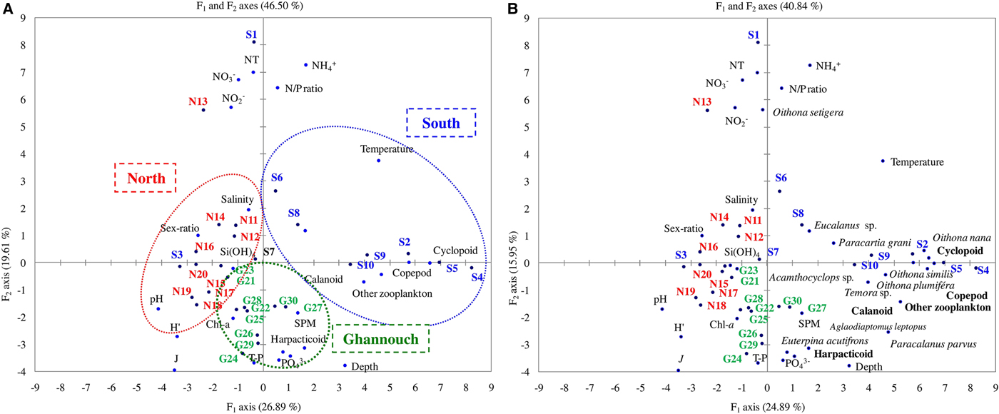
Fig. 6. Canonical correspondence analysis (CCA) (Axis I and II) on mean values of several physical and chemical parameters with (A) zooplankton group and (B) copepod species in stations sampled in the northern and southern coastal areas of Sfax and the Ghannouch area sampled during autumn (October–November 2014).
DISCUSSION
Zooplankton is recognized among the best indicators for investigating and documenting environmental changes (Siokou-Frangou & Papathanassiou, Reference Siokou-Frangou and Papathanassiou1991; Sipkay et al., Reference Sipkay, Kiss, Vadadi-Fülöp and Hufnagel2009; Bagheri et al., Reference Bagheri, Sabkara, Mirzajani, Khodaparast, Yosefzad and Yeok2013). The variations of zooplankton populations are closely related to environmental parameters such as temperature, pH and salinity (Pascual & Guichard, Reference Pascual and Guichard2005; Rossi & Jamet, Reference Rossi, Jamet, Martorino and Puopolo2009; Srichandan et al., Reference Srichandan, Panda and Rout2013). Main zooplankton taxa have short life cycles and their community structure is able to reflect real-time scenarios as it is less enforced by the stability of individuals from previous years (Richardson, Reference Richardson2008; Bagheri et al., Reference Bagheri, Sabkara, Mirzajani, Khodaparast, Yosefzad and Yeok2013). Thus, hypoxic/anoxic conditions related to organic enrichment are found to be associated with the decrease of zooplankton abundance in eutrophic and/or organically polluted systems (Stalder & Marcus, Reference Stalder and Marcus1997; Park & Marshall, Reference Park and Marshall2000; Gordina et al., Reference Gordina, Pavlova, Ovsyany, Wilson, Kemp and Romanov2001) and high turbidity can increase the death rate of copepods (e.g. Castel & Feurtet, Reference Castel and Feurtet1992).
Anthropogenic inputs status of the coastal zone
We found quite high PO43− concentrations, very probably related to inputs from the phosphate processing industries (SIAPE-Sfax and GCT-Gabes), revealing different anthropogenic input degrees. In this context, we may say that GA is the most affected by PO43− followed by SC and NC. The high concentration of PO43− (4.46 ± 2.60 µm) in GA was in the range of values previously reported by Baccar (Reference Baccar2014) in the Gabes area (3.73 ± 1.57 µm), while the values we found at SC (3.11 ± 2.81 µm) and NC (2.07 ± 0.62 µm) were far higher than the ones noted by Rekik et al. (Reference Rekik, Drira, Guermazi, Elloumi, Maalej, Aleya and Ayadi2012) (0.28 ± 0.05 µm) in SC or by Drira et al. (Reference Drira, Bel Hassen, Hamza, Rebai, Bouain, Ayadi and Aleya2009) in the offshore waters of the Gulf of Gabes (0.06 ± 0.03 µm). The highest levels of PO43−were always found near the potential sources, i.e. the SIAPE-Sfax plant (station 4), wadi El Maou (station 7), the Sfax fishing harbour (station 9) and the commercial harbour (stations 25 and 27) and the GCT-Gabes phosphoric acid industry (station 28) for GA. Therefore, the high apparent availability of inorganic phosphates in the SC and GA areas were related to the release of phosphate residues from the SIAPE and GCT-Gabes industries (Bejaoui et al., Reference Bejaoui, Raïs and Koutitonsky2004; Ben Brahim et al., Reference Ben Brahim, Hamza, Hannachi, Rebai, Jarboui, Bouain and Aleya2010; Rekik et al., Reference Rekik, Drira, Guermazi, Elloumi, Maalej, Aleya and Ayadi2012; Ben Salem et al., Reference Ben Salem, Drira and Ayadi2015; Drira et al., Reference Drira, Kmiha-Megdiche, Sahnoun, Hammami, Allouche, Tedetti and Ayadi2016). Ammonium, which was the chemical factor with the most significant differences between areas, showed the highest value in the SC (ANOVA, P < 0.001). The importance of ammonium compared with nitrite and nitrate was a typical finding of coastal eutrophic waters due to anthropogenic pollution, mainly represented by untreated discharges (Nuccio et al., Reference Nuccio, Melillo, Massi and Innamorati2003; Bouchouicha-Smida et al., Reference Bouchouicha-Smida, Sahraoui, Mabrouk and Sakka Hlaili2012). Our result also showed that NC was slightly alkaline (pH 8.12 ± 0.06) compared with GA (pH = 8.05 ± 0.07), and SC (pH = 7.99 ± 0.07), which is in agreement with results reported by Rekik et al. (Reference Rekik, Maalej, Ayadi and Aleya2013) at the same season (8.16 ± 0.3) for this area.
Copepod assemblages as a bioindicator of environmental quality
Investigations on zooplankton community in relation with anthropogenic inputs have already been conducted in the Mediterranean Sea (Siokou-Frangou, Reference Siokou-Frangou1996; Jamet et al., Reference Jamet, Boge, Richard, Geneys and Jamet2001; Isinibilir et al., Reference Isinibilir, Kideys, Tarkan and Yilmaz2008; Papantoniou et al., Reference Papantoniou, Danielidis, Spyropoulou and Ragopoulu2015). One previous study has been performed so far in the coastal waters of the Gulf of Gabes, i.e. in the SC (Drira et al., submitted). In this study, we tried to determine the effects of anthropogenic inputs on planktonic copepods by comparing the abundance and spatial distribution of the main species in three coastal marine areas with different anthropogenic input levels. Our results showed a clear dominance of copepods (nauplii stage to the adult stage) in the three areas, representing 76, 83 and 84% of total zooplankton in GA, SC and NC, respectively. The dominance of copepods has already been reported in several studies in the Gulf of Gabes: in SC (5–50%; Ben Salem et al., Reference Ben Salem, Drira and Ayadi2015), NC (82%, Rekik et al., Reference Rekik, Drira, Guermazi, Elloumi, Maalej, Aleya and Ayadi2012), in the city of Gabes: Ghannouch and Zarrat (46–83%; Baccar, Reference Baccar2014) and in offshore waters of the Gulf of Gabes (83%; Drira et al., Reference Drira, Bel Hassen, Ayadi and Aleya2014; Ben Ltaief et al., Reference Ben Ltaief, Drira, Hannachi, Bel Hassen, Hamza, Pagano and Ayadi2015).
In this study, we reported the presence of 25 species belonging to 13 families and three orders, namely calanoid, cyclopoid and harpacticoid, while poecilostomatoid were virtually absent. We found a preponderance of cyclopoids, particularly in SC (with 80% of total copepod abundance), while calanoids were also important in GA (51%) and NC (43%). This is consistent with previous works showing that cyclopoids are numerically the most important group in the Gulf of Gabes (Drira et al., Reference Drira, Bel Hassen, Hamza, Rebai, Bouain, Ayadi and Aleya2009, Reference Drira, Bel Hassen, Ayadi and Aleya2014; Ben Ltaief et al., Reference Ben Ltaief, Drira, Hannachi, Bel Hassen, Hamza, Pagano and Ayadi2015). This predominance of cyclopoids in such polluted areas agrees with their cosmopolitan and less demanding character in terms of environmental conditions compared with other groups (Sarkka et al., Reference Sarkka, Levonen and Mäkelä1998). Adult copepods dominated other developmental stages of copepods in the three study sites with adult females being predominant (>58% of adults). The dominance of females was already reported in the Gulf of Gabes (2005–2007) (Drira et al., Reference Drira, Bel Hassen, Ayadi, Hamza, Zarrad, Bouaïn and Aleya2010a, Reference Drira, Hamza, Bel Hassen, Ayadi, Bouaïn and Aleyab, Reference Drira, Bel Hassen, Ayadi and Aleya2014). Dominance of females compared with males, which reduces the sex ratio (Kiorboe, Reference Kiorboe2006), may be due to the higher mortality of males because of their increased vulnerability to predation during their search for mates (Mendes-Gusmão et al., Reference Mendes-Gusmão, McKinnon and Richardson2013). In addition, environmental factors such as pollution have strong effects on copepod sex ratio, and suggest that differential physiological longevity of males and females may be more important in determining the sex ratio (Mendes-Gusmão et al., Reference Mendes-Gusmão, McKinnon and Richardson2013). Oithonids were numerically very important with O. nana (36% of zooplankton abundance in SC, 12.7% in NC and 6.4% in GA and O. similis (23% in SC, 21% in NC and 17% in GA) as the main species. In previous studies, O. nana were also reported at a very high abundance in SC (Drira et al., submitted) as well as in NC before (2007; Rekik et al., Reference Rekik, Drira, Guermazi, Elloumi, Maalej, Aleya and Ayadi2012) and after (2009–2010; Rekik et al., Reference Rekik, Maalej, Ayadi and Aleya2013) the Taparura restoration process. In the CCA analysis, Oithonids (and O. similis) were negatively correlated with the NC stations corresponding to the less disturbed area and positively correlated with the polluted SC stations, which clearly indicates an affinity of these copepods for anthropogenic inputs. In general, oithonidae may survive in a wide range of habitats and maintain their populations under adverse conditions because they are morphologically less specialized than calanoids (Paffenhöfer, Reference Paffenhöfer1993). In agreement with our study, Oithonidae, and more specifically O. nana, are often associated with a high degree of anthropogenic inputs and regarded as a bio-indicator species of anthropogenic pollution (Annabi-Trabelsi et al., Reference Annabi-Trabelsi, Daly-Yahia, Romdhane and Ben-Maïz2005; Drira et al., Reference Drira, Bel Hassen, Ayadi and Aleya2014; Serranito et al., Reference Serranito, Aubert, Stemmann, Rossi and Jamet2016). The good adaptation of O. nana to anthropized areas can be partly explained by its feeding habits (Serranito et al., Reference Serranito, Aubert, Stemmann, Rossi and Jamet2016). It has been reported to be more flexible in its diet compared with other copepods, thus able to adapt to a wide range of food resources (Moraitou-Apostolopoulou, Reference Moraitou-Apostolopoulou1976; Lampitt & Gamble, Reference Lampitt and Gamble1982; Rekik et al., Reference Rekik, Drira, Guermazi, Elloumi, Maalej, Aleya and Ayadi2012; Serranito et al., Reference Serranito, Aubert, Stemmann, Rossi and Jamet2016) and having a mixotrophic diet by incorporating faecal matter, ciliates protozoa and dinoflagellates (Williams & Muxagata, Reference Williams and Muxagata2006). This small euryoecious species is characterized by a high tolerance to various environmental parameters (Riccardi & Mariotto, Reference Riccardi and Mariotto2000). Its shorter life cycle and higher reproduction rate compared with larger copepods could also partly explain its higher success in adapting to new conditions (Gallienne & Robins, Reference Gallienne and Robins2001). Oithona similis is a ubiquitous and abundant cyclopoid not only in our study site, but also in the Algerian basin (Riandey et al., Reference Riandey, Champalbert, Carlotti, Taupier-Letage and Thibault-Botha2005), in the Bay of Tunis (Daly-Yahia et al., Reference Daly-Yahia, Souissi and Daly-Yahia Kéfi2004), in the lagoon of Tunis (Annabi-Trabelsi et al., Reference Annabi-Trabelsi, Daly-Yahia, Romdhane and Ben-Maïz2005) and in the offshore waters of the Gulf of Gabes (Drira et al., Reference Drira, Bel Hassen, Hamza, Rebai, Bouain, Ayadi and Aleya2009). In our study, harpacticoid and more specifically Euterpina acutifrons, were clearly associated to highly polluted conditions as they were correlated to GA stations characterized by the highest SPM and PO43− concentrations. Euterpina acutifrons, known as eurythermic and euryhaline, lives in marine coastal areas (Furnestin, Reference Furnestin1960; Moreira et al., Reference Moreira, Jillett, Vernberg and Weinrich1982; Delia Vinas et al., Reference Delia Vinas, Diovisalvi and Cepeda2010). The plasticity of this species which occupies several coastal habitats is often due to its broad trophic spectrum (phytoplankton, microplankton and detritus) (Goswani, Reference Goswani1976; Moreira et al., Reference Moreira, Yamashita and McNamara1983).
The taxonomic diversity is also strongly influenced by anthropogenic inputs (Danilov & Ekelund, Reference Danilov and Ekelund1999). In the present work, we showed that NC, considered as a restored environment in term of phosphogypsum contamination, was characterized by a taxonomic diversity (H′ = 1.95 bits ind−1, J′ = 0.6) higher than in GA (H′ = 1.74 bits ind−1, J′ = 0.6) and SC (H′ = 1.49 bits ind−1, J′ = 0.5). Taxonomic diversity (as Piélou's evenness) as well as Oithonidae relative abundance were singled out as the most pertinent indicators of anthropogenic pollution in the case study of the Bay of Toulon (Mediterranean Sea) (Serranito et al., Reference Serranito, Aubert, Stemmann, Rossi and Jamet2016). In our study, based on the same indicators we could classify the three study sites according to the significance of pollution impact on copepods as follows: NC < GA < SC with the diversity (H′ = 1.95, 1.74 and 1.49 bits ind−1, respectively), and GA < NC < SC with the percentage of oithonidae (43, 51 and 79%, respectively). We can also note that the mean Indicator Values for Oithonidae are also higher for the SC area (48%) than for NC and GA (3.7 and 12.2% respectively), which is consistent with the indicator based on this copepod family. In this context, we may assume that GA, although the most affected by orthophosphates (4.46 ± 2.60 µm) is a more pollution-resistant ecosystem than SC (3.11 ± 2.81 µm) compared with NC (2.07 ± 0.62 µm).
CONCLUSION
This study was undertaken to assess the zooplankton communities in accordance with anthropogenic inputs in the Sfax northern and southern coasts and in the Ghannouch area during October and November 2014. These three areas were characterized by different degrees of anthropogenic inputs characterized by levels of PO43− with highest values at GA (stations 25 and 27 near the commercial harbour and station 28 in front of GCT-Gabes) and lowest at NC. The most abundant species in the three environments were O. nana, O. similis and Paracalanus parvus while two species were reported for the first time in the Gulf of Gabes (Aglaodiaptomus leptopus and Eucalanus sp.). Oithona nana and O. similis could be used as an indicator of anthropogenic inputs in the Gulf of Gabes. Our results indicate that the fluctuation of copepod abundances may be a useful tool to evaluate the ecosystem health status. The present work shows that the Northern coast, considered as a restored and reclaimed environment, is characterized by slightly higher species diversity, while the Ghannouch area, although the most affected by orthophosphates, was found to be more pollution-resistant than the southern coast. Meanwhile, our study can be useful in the management of this ecosystem for planning the best disposal options for treating urban and industrial wastes in the gulf's coastal waters.
ACKNOWLEDGEMENTS
This work was conducted in the Biodiversity and Aquatic Ecosystems UR/11ES72 Research Unit at the University of Sfax in collaboration with the Mediterranean Institute of Oceanography (MIO) Marseille, France. This work was carried out in the framework of the IRD Action South project ‘MANGA’ and the IRD French-Tunisian International Joint Laboratory (LMI) ‘COSYS-Med’ This work is a contribution of the WP3 C3A-Action MERMEX/MISTRALS. This study was carried out in the framework of the postdoctoral fellowship of Z. Drira (University of Sfax, Tunisia). The authors acknowledge Mr T. Omar and Mr H. Sahnoun for their technical help during the cruise. We thank the core parameter analytical platform (PAPB) of the MIO for performing analyses of chl-a, Phaeo-a, POC and PON. Special thanks are also due to Mr K. Maaloul, translator and English professor at the Sfax Faculty of Sciences, University of Sfax (Sfax, Tunisia) for constructive proofreading and language improving services.


