


1 Introduction
Any study of propagating shock waves in interplanetary space requires knowledge of the characteristic physical parameters of the shock including the shock velocity, the upstream Mach number, the type of shock, etc. These parameters are usually determined by somehow ‘fitting’ the experimental data to the simplest conceivable model of an ideal MHD shock consisting of a planar shock front – a surface of discontinuity – propagating with constant velocity
 $\boldsymbol{V}_{\text{sh}}$
through an ideal (inviscid and perfectly conducting) magnetohydrodynamic (MHD) fluid in which the plasma states upstream and downstream are both constant, independent of time (Sonett et al.
Reference Sonett, Colburn, Davis, Smith and Coleman1964; Colburn & Sonett Reference Colburn and Sonett1966; Chao Reference Chao1970; Hudson Reference Hudson1970). Within this theoretical framework, changes in the mass density, magnetic field and other plasma variables across the shock surface must satisfy the Rankine–Hugoniot relations of ideal MHD, also called the ‘jump conditions’ of ideal MHD. By fitting solar wind data to the jump conditions in various ways, measurements of the plasma states upstream and downstream of interplanetary shocks have been used to estimate the shock velocity
$\boldsymbol{V}_{\text{sh}}$
through an ideal (inviscid and perfectly conducting) magnetohydrodynamic (MHD) fluid in which the plasma states upstream and downstream are both constant, independent of time (Sonett et al.
Reference Sonett, Colburn, Davis, Smith and Coleman1964; Colburn & Sonett Reference Colburn and Sonett1966; Chao Reference Chao1970; Hudson Reference Hudson1970). Within this theoretical framework, changes in the mass density, magnetic field and other plasma variables across the shock surface must satisfy the Rankine–Hugoniot relations of ideal MHD, also called the ‘jump conditions’ of ideal MHD. By fitting solar wind data to the jump conditions in various ways, measurements of the plasma states upstream and downstream of interplanetary shocks have been used to estimate the shock velocity
 $\boldsymbol{V}_{\text{sh}}$
(see, for example, Sonett et al.
Reference Sonett, Colburn, Davis, Smith and Coleman1964; Ogilvie & Burlaga Reference Ogilvie and Burlaga1969; Lepping & Argentiero Reference Lepping and Argentiero1971; Abraham-Shrauner & Yun Reference Abraham-Shrauner and Yun1976; Russell et al.
Reference Russell, Mellott, Smith and King1983; Hsieh & Richter Reference Hsieh and Richter1986; Viñas & Scudder Reference Viñas and Scudder1986; Szabo Reference Szabo1994; Balogh & Riley Reference Balogh, Riley, Jokipii, Sonett and Giampapa1997; Berdichevsky et al.
Reference Berdichevsky, Szabo, Lepping, Viñas and Mariani2000; Oh, Yi & Kim Reference Oh, Yi and Kim2007). This approach requires that the MHD jump conditions used in the fitting procedure are sufficient to uniquely determine the shock velocity, both speed and direction, given the plasma parameters upstream and downstream of the shock.
$\boldsymbol{V}_{\text{sh}}$
(see, for example, Sonett et al.
Reference Sonett, Colburn, Davis, Smith and Coleman1964; Ogilvie & Burlaga Reference Ogilvie and Burlaga1969; Lepping & Argentiero Reference Lepping and Argentiero1971; Abraham-Shrauner & Yun Reference Abraham-Shrauner and Yun1976; Russell et al.
Reference Russell, Mellott, Smith and King1983; Hsieh & Richter Reference Hsieh and Richter1986; Viñas & Scudder Reference Viñas and Scudder1986; Szabo Reference Szabo1994; Balogh & Riley Reference Balogh, Riley, Jokipii, Sonett and Giampapa1997; Berdichevsky et al.
Reference Berdichevsky, Szabo, Lepping, Viñas and Mariani2000; Oh, Yi & Kim Reference Oh, Yi and Kim2007). This approach requires that the MHD jump conditions used in the fitting procedure are sufficient to uniquely determine the shock velocity, both speed and direction, given the plasma parameters upstream and downstream of the shock.
Uniqueness is not at all obvious since the jump conditions form a nonlinear system of equations for
 $\boldsymbol{V}_{\text{sh}}$
that has more equations than unknowns and because there exist three different types of MHD shocks (slow, intermediate and fast) with distinctly different physical properties. To this author’s knowledge a mathematical proof that the solution for
$\boldsymbol{V}_{\text{sh}}$
that has more equations than unknowns and because there exist three different types of MHD shocks (slow, intermediate and fast) with distinctly different physical properties. To this author’s knowledge a mathematical proof that the solution for
 $\boldsymbol{V}_{\text{sh}}$
is unique has never been given. The purpose of this paper is to show that the jump conditions of ideal MHD uniquely determine the shock velocity for any and all types of MHD shocks and to investigate the minimum number of jump conditions required to accomplish this. For simplicity, this study is restricted to the case of an ideal MHD medium with an isotropic pressure tensor.
$\boldsymbol{V}_{\text{sh}}$
is unique has never been given. The purpose of this paper is to show that the jump conditions of ideal MHD uniquely determine the shock velocity for any and all types of MHD shocks and to investigate the minimum number of jump conditions required to accomplish this. For simplicity, this study is restricted to the case of an ideal MHD medium with an isotropic pressure tensor.
Jump conditions containing pressure terms are relatively complex and more difficult to evaluate accurately using experimental data, contrary to jump conditions that are independent of the pressure; this is especially true when the pressure tensor is anisotropic. This suggests that, statistically, methods based solely on those jump conditions that are independent of the pressure should give more accurate results. Such methods have been utilized by Lepping & Argentiero (Reference Lepping and Argentiero1971), Viñas & Scudder (Reference Viñas and Scudder1986) and possibly others. When the pressure tensor is anisotropic there are three and only three jump conditions that are independent of the plasma pressure: the conservation of mass flux through the shock, the continuity of the normal component of the magnetic field and the continuity of the tangential electric field in the frame of reference of the shock. These three conditions reduce to three scalar equations, however, two of the three scalar equations are degenerate (equivalent) and, therefore, these three equations are insufficient to uniquely determine the shock velocity
 $\boldsymbol{V}_{\text{sh}}$
in terms of the plasma states upstream and downstream. In fact, these equations possess an infinite continuum of possible solutions
$\boldsymbol{V}_{\text{sh}}$
in terms of the plasma states upstream and downstream. In fact, these equations possess an infinite continuum of possible solutions
When the pressure tensor is isotropic, there is a fourth jump condition that is independent of the pressure, namely, the continuity of the tangential component of the momentum flux. When combined with the three jump conditions mentioned in the last paragraph, these four jump conditions reduce to four scalar equations. In this case, however, three of the four equations are degenerate (equivalent) so they too are insufficient to uniquely determine the shock velocity
 $\boldsymbol{V}_{\text{sh}}$
. Consequently, for the simple planar ideal MHD shock model considered here it is mathematically impossible to uniquely determine the shock velocity
$\boldsymbol{V}_{\text{sh}}$
. Consequently, for the simple planar ideal MHD shock model considered here it is mathematically impossible to uniquely determine the shock velocity
 $\boldsymbol{V}_{\text{sh}}$
from the MHD jump conditions without using at least one jump condition containing the pressure. The same is true when the pressure tensor is anisotropic. In general, at least three different scalar equations are required to uniquely determine the three components of the vector
$\boldsymbol{V}_{\text{sh}}$
from the MHD jump conditions without using at least one jump condition containing the pressure. The same is true when the pressure tensor is anisotropic. In general, at least three different scalar equations are required to uniquely determine the three components of the vector
 $\boldsymbol{V}_{\text{sh}}$
from measured data. Remarkably, in the case of MHD media characterized by a scalar pressure, even though the jump condition for the pressure is necessary to derive the theoretical results, it turns out that measurements of the pressure are not necessary for the experimental determination of
$\boldsymbol{V}_{\text{sh}}$
from measured data. Remarkably, in the case of MHD media characterized by a scalar pressure, even though the jump condition for the pressure is necessary to derive the theoretical results, it turns out that measurements of the pressure are not necessary for the experimental determination of
 $\boldsymbol{V}_{\text{sh}}$
.
$\boldsymbol{V}_{\text{sh}}$
.
2 Jump conditions
In ideal MHD, the conservation of mass flux across the shock surface, the continuity of the normal component of the magnetic field and the continuity of the tangential electric field in the frame of reference of the shock may be written, respectively,
 $$\begin{eqnarray}\displaystyle & \displaystyle \unicode[STIX]{x1D70C}_{1}(\boldsymbol{V}_{1}-\boldsymbol{V}_{\text{sh}})\boldsymbol{\cdot }\hat{\boldsymbol{n}}=\unicode[STIX]{x1D70C}_{2}(\boldsymbol{V}_{2}-\boldsymbol{V}_{\text{sh}})\boldsymbol{\cdot }\hat{\boldsymbol{n}}, & \displaystyle\end{eqnarray}$$
 $$\begin{eqnarray}\displaystyle & \displaystyle \boldsymbol{B}_{1}\boldsymbol{\cdot }\hat{\boldsymbol{n}}=\boldsymbol{B}_{2}\boldsymbol{\cdot }\hat{\boldsymbol{n}}, & \displaystyle\end{eqnarray}$$
 $$\begin{eqnarray}\displaystyle & \displaystyle \hat{\boldsymbol{n}}\times [(\boldsymbol{V}_{1}-\boldsymbol{V}_{\text{sh}})\times \boldsymbol{B}_{1}]=\hat{\boldsymbol{n}}\times [(\boldsymbol{V}_{2}-\boldsymbol{V}_{\text{sh}})\times \boldsymbol{B}_{2}], & \displaystyle\end{eqnarray}$$
where
 $\boldsymbol{V}$
is the plasma flow velocity,
$\boldsymbol{V}$
is the plasma flow velocity,
 $\unicode[STIX]{x1D70C}$
is the mass density,
$\unicode[STIX]{x1D70C}$
is the mass density,
 $\boldsymbol{B}$
is the plasma magnetic field,
$\boldsymbol{B}$
is the plasma magnetic field,
 $\hat{\boldsymbol{n}}$
is the unit normal to the shock surface, and the subscripts ‘1’ and ‘2’ denote the regions on opposite sides of the shock. Jump condition (2.2) says that the vector
$\hat{\boldsymbol{n}}$
is the unit normal to the shock surface, and the subscripts ‘1’ and ‘2’ denote the regions on opposite sides of the shock. Jump condition (2.2) says that the vector
 $\unicode[STIX]{x0394}\boldsymbol{B}=\boldsymbol{B}_{1}-\boldsymbol{B}_{2}$
is tangent to the shock surface. Using the vector identity
$\unicode[STIX]{x0394}\boldsymbol{B}=\boldsymbol{B}_{1}-\boldsymbol{B}_{2}$
is tangent to the shock surface. Using the vector identity
 $\boldsymbol{A}\times (\boldsymbol{B}\times \boldsymbol{C})=(\boldsymbol{A}\boldsymbol{\cdot }\boldsymbol{C})\boldsymbol{B}-(\boldsymbol{A}\boldsymbol{\cdot }\boldsymbol{B})\boldsymbol{C}$
, equation (2.3) becomes
$\boldsymbol{A}\times (\boldsymbol{B}\times \boldsymbol{C})=(\boldsymbol{A}\boldsymbol{\cdot }\boldsymbol{C})\boldsymbol{B}-(\boldsymbol{A}\boldsymbol{\cdot }\boldsymbol{B})\boldsymbol{C}$
, equation (2.3) becomes
 $$\begin{eqnarray}(\boldsymbol{B}_{1}\boldsymbol{\cdot }\hat{\boldsymbol{n}})(\boldsymbol{V}_{1}-\boldsymbol{V}_{\text{sh}})-\boldsymbol{B}_{1}(\boldsymbol{V}_{1}-\boldsymbol{V}_{\text{sh}})\boldsymbol{\cdot }\hat{\boldsymbol{n}}=(\boldsymbol{B}_{2}\boldsymbol{\cdot }\hat{\boldsymbol{n}})(\boldsymbol{V}_{2}-\boldsymbol{V}_{\text{sh}})-\boldsymbol{B}_{2}(\boldsymbol{V}_{2}-\boldsymbol{V}_{\text{sh}})\boldsymbol{\cdot }\hat{\boldsymbol{n}}.\end{eqnarray}$$
Using (2.1) and (2.2), the continuity of the tangential electric field (2.4) reduces to
 $$\begin{eqnarray}(\boldsymbol{V}_{1}-\boldsymbol{V}_{2})(\boldsymbol{B}_{1}\boldsymbol{\cdot }\hat{\boldsymbol{n}})=\left(\frac{\boldsymbol{B}_{1}}{\unicode[STIX]{x1D70C}_{1}}-\frac{\boldsymbol{B}_{2}}{\unicode[STIX]{x1D70C}_{2}}\right)[\unicode[STIX]{x1D70C}_{1}(\boldsymbol{V}_{1}-\boldsymbol{V}_{\text{sh}})\boldsymbol{\cdot }\hat{\boldsymbol{n}}].\end{eqnarray}$$
For non-perpendicular shocks
 $\boldsymbol{B}_{1}\boldsymbol{\cdot }\hat{\boldsymbol{n}}\neq 0$
and
$\boldsymbol{B}_{1}\boldsymbol{\cdot }\hat{\boldsymbol{n}}\neq 0$
and
 $\unicode[STIX]{x1D70C}_{1}(\boldsymbol{V}_{1}-\boldsymbol{V}_{\text{sh}})\boldsymbol{\cdot }\hat{\boldsymbol{n}}\neq 0$
and, in this case, it follows from (2.5) that
$\unicode[STIX]{x1D70C}_{1}(\boldsymbol{V}_{1}-\boldsymbol{V}_{\text{sh}})\boldsymbol{\cdot }\hat{\boldsymbol{n}}\neq 0$
and, in this case, it follows from (2.5) that
 $$\begin{eqnarray}\boldsymbol{V}_{1}-\boldsymbol{V}_{2}\propto \frac{\boldsymbol{B}_{1}}{\unicode[STIX]{x1D70C}_{1}}-\frac{\boldsymbol{B}_{2}}{\unicode[STIX]{x1D70C}_{2}}.\end{eqnarray}$$
Thus, for non-perpendicular shocks the vector relations (2.5) and (2.6) hold and (2.5) reduces to the scalar equation
 $$\begin{eqnarray}|\boldsymbol{V}_{1}-\boldsymbol{V}_{2}|^{2}(\boldsymbol{B}_{1}\boldsymbol{\cdot }\hat{\boldsymbol{n}})=(\boldsymbol{V}_{1}-\boldsymbol{V}_{2})\boldsymbol{\cdot }\left(\frac{\boldsymbol{B}_{1}}{\unicode[STIX]{x1D70C}_{1}}-\frac{\boldsymbol{B}_{2}}{\unicode[STIX]{x1D70C}_{2}}\right)[\unicode[STIX]{x1D70C}_{1}(\boldsymbol{V}_{1}-\boldsymbol{V}_{\text{sh}})\boldsymbol{\cdot }\hat{\boldsymbol{n}}].\end{eqnarray}$$
For purposes of numerical calculations with experimental data it is preferable to rewrite (2.7) in a form similar to (2.1) and (2.2), a form that is invariant under the interchange of the indices 1 and 2, that is, in the form
 $$\begin{eqnarray}\displaystyle & & \displaystyle |\boldsymbol{V}_{1}-\boldsymbol{V}_{2}|^{2}(\boldsymbol{B}_{1}+\boldsymbol{B}_{2})\boldsymbol{\cdot }\hat{\boldsymbol{n}}\nonumber\\ \displaystyle & & \displaystyle \quad =(\boldsymbol{V}_{1}-\boldsymbol{V}_{2})\boldsymbol{\cdot }\left(\frac{\boldsymbol{B}_{1}}{\unicode[STIX]{x1D70C}_{1}}-\frac{\boldsymbol{B}_{2}}{\unicode[STIX]{x1D70C}_{2}}\right)[\unicode[STIX]{x1D70C}_{1}(\boldsymbol{V}_{1}-\boldsymbol{V}_{\text{sh}})+\unicode[STIX]{x1D70C}_{2}(\boldsymbol{V}_{2}-\boldsymbol{V}_{\text{sh}})]\boldsymbol{\cdot }\hat{\boldsymbol{n}}.\end{eqnarray}$$
If the plasma states upstream and downstream are known, then the three jump conditions (2.1), (2.2) and (2.8) form a system of three scalar equations in the three unknown components of the vector
 $\boldsymbol{V}_{\text{sh}}$
. For a medium with a pressure tensor that is either isotropic or gyrotropic with respect to the direction of the magnetic field
$\boldsymbol{V}_{\text{sh}}$
. For a medium with a pressure tensor that is either isotropic or gyrotropic with respect to the direction of the magnetic field
 $\boldsymbol{B}$
, this nonlinear system of equations is degenerate and, therefore, it does not possess a unique non-trivial solution (see the next section). This result is a consequence of the so called coplanarity theorem which says that the tangential components of
$\boldsymbol{B}$
, this nonlinear system of equations is degenerate and, therefore, it does not possess a unique non-trivial solution (see the next section). This result is a consequence of the so called coplanarity theorem which says that the tangential components of
 $\boldsymbol{B}_{1}$
,
$\boldsymbol{B}_{1}$
,
 $\boldsymbol{B}_{2}$
and
$\boldsymbol{B}_{2}$
and
 $\unicode[STIX]{x0394}\boldsymbol{V}$
are colinear (Landau & Lifshitz Reference Landau and Lifshitz1960; Colburn & Sonett Reference Colburn and Sonett1966). On the other hand, if the pressure anisotropy is such that the coplanarity theorem does not hold, then the system of three scalar equations (2.1), (2.2) and (2.8) may not be degenerate. Whether this type of pressure anisotropy exists in the solar wind is an interesting question. In the solar wind there are clearly two preferred directions: the magnetic field direction and, as a consequence of the radial expansion, the radial direction. Therefore, non-gyrotropic pressure anisotropies likely exist although they shall not be considered here.
$\unicode[STIX]{x0394}\boldsymbol{V}$
are colinear (Landau & Lifshitz Reference Landau and Lifshitz1960; Colburn & Sonett Reference Colburn and Sonett1966). On the other hand, if the pressure anisotropy is such that the coplanarity theorem does not hold, then the system of three scalar equations (2.1), (2.2) and (2.8) may not be degenerate. Whether this type of pressure anisotropy exists in the solar wind is an interesting question. In the solar wind there are clearly two preferred directions: the magnetic field direction and, as a consequence of the radial expansion, the radial direction. Therefore, non-gyrotropic pressure anisotropies likely exist although they shall not be considered here.
It follows from (2.1) that
 $$\begin{eqnarray}V_{\text{sh}}=\frac{(\unicode[STIX]{x1D70C}_{1}\boldsymbol{V}_{1}-\unicode[STIX]{x1D70C}_{2}\boldsymbol{V}_{2})}{\unicode[STIX]{x1D70C}_{1}-\unicode[STIX]{x1D70C}_{2}}\boldsymbol{\cdot }\hat{\boldsymbol{n}},\end{eqnarray}$$
from (2.7) that
 $$\begin{eqnarray}V_{\text{sh}}=\left[\boldsymbol{V}_{1}-\frac{|\unicode[STIX]{x0394}\boldsymbol{V}|^{2}}{\unicode[STIX]{x0394}\boldsymbol{V}\boldsymbol{\cdot }\unicode[STIX]{x0394}(\boldsymbol{B}/\unicode[STIX]{x1D70C})}\left(\frac{\boldsymbol{B}_{1}}{\unicode[STIX]{x1D70C}_{1}}\right)\right]\boldsymbol{\cdot }\hat{\boldsymbol{n}}\end{eqnarray}$$
and
 $$\begin{eqnarray}V_{\text{sh}}=\left[\boldsymbol{V}_{2}-\frac{|\unicode[STIX]{x0394}\boldsymbol{V}|^{2}}{\unicode[STIX]{x0394}\boldsymbol{V}\boldsymbol{\cdot }\unicode[STIX]{x0394}(\boldsymbol{B}/\unicode[STIX]{x1D70C})}\left(\frac{\boldsymbol{B}_{2}}{\unicode[STIX]{x1D70C}_{2}}\right)\right]\boldsymbol{\cdot }\hat{\boldsymbol{n}},\end{eqnarray}$$
and from (2.8) that
 $$\begin{eqnarray}V_{\text{sh}}=\left[\frac{\unicode[STIX]{x1D70C}_{1}\boldsymbol{V}_{1}+\unicode[STIX]{x1D70C}_{2}\boldsymbol{V}_{2}}{\unicode[STIX]{x1D70C}_{1}+\unicode[STIX]{x1D70C}_{2}}-\frac{|\unicode[STIX]{x0394}\boldsymbol{V}|^{2}}{\unicode[STIX]{x0394}\boldsymbol{V}\boldsymbol{\cdot }\unicode[STIX]{x0394}(\boldsymbol{B}/\unicode[STIX]{x1D70C})}\left(\frac{\boldsymbol{B}_{1}+\boldsymbol{B}_{2}}{\unicode[STIX]{x1D70C}_{1}+\unicode[STIX]{x1D70C}_{2}}\right)\right]\boldsymbol{\cdot }\hat{\boldsymbol{n}}.\end{eqnarray}$$
Another form that is invariant under interchange of the indices is
 $$\begin{eqnarray}V_{\text{sh}}=\left[\frac{\boldsymbol{V}_{1}+\boldsymbol{V}_{2}}{2}-\frac{|\unicode[STIX]{x0394}\boldsymbol{V}|^{2}}{\unicode[STIX]{x0394}\boldsymbol{V}\boldsymbol{\cdot }\unicode[STIX]{x0394}(\boldsymbol{B}/\unicode[STIX]{x1D70C})}\left(\frac{\boldsymbol{B}_{1}+\boldsymbol{B}_{2}}{2}\right)\right]\boldsymbol{\cdot }\hat{\boldsymbol{n}}.\end{eqnarray}$$
Alternative expressions are
 $$\begin{eqnarray}V_{\text{sh}}=\left[\boldsymbol{V}_{1}-\frac{\unicode[STIX]{x0394}\boldsymbol{V}\boldsymbol{\cdot }\unicode[STIX]{x0394}(\boldsymbol{B}/\unicode[STIX]{x1D70C})}{|\unicode[STIX]{x0394}(\boldsymbol{B}/\unicode[STIX]{x1D70C})|^{2}}\left(\frac{\boldsymbol{B}_{1}}{\unicode[STIX]{x1D70C}_{1}}\right)\right]\boldsymbol{\cdot }\hat{\boldsymbol{n}},\end{eqnarray}$$
and
 $$\begin{eqnarray}V_{\text{sh}}=\left[\frac{\boldsymbol{V}_{1}+\boldsymbol{V}_{2}}{2}-\frac{\unicode[STIX]{x0394}\boldsymbol{V}\boldsymbol{\cdot }\unicode[STIX]{x0394}(\boldsymbol{B}/\unicode[STIX]{x1D70C})}{|\unicode[STIX]{x0394}(\boldsymbol{B}/\unicode[STIX]{x1D70C})|^{2}}\left(\frac{\boldsymbol{B}_{1}+\boldsymbol{B}_{2}}{2}\right)\right]\boldsymbol{\cdot }\hat{\boldsymbol{n}},\end{eqnarray}$$
etc. The expressions (2.10)–(2.15) do not appear to have been noted previously.
3 How to construct the solution
To find the solutions of the system (2.1), (2.2), and (2.8) let
 $\hat{\boldsymbol{\unicode[STIX]{x1D702}}}$
be any vector perpendicular to
$\hat{\boldsymbol{\unicode[STIX]{x1D702}}}$
be any vector perpendicular to
 $\unicode[STIX]{x0394}\boldsymbol{B}=\boldsymbol{B}_{1}-\boldsymbol{B}_{2}$
such that
$\unicode[STIX]{x0394}\boldsymbol{B}=\boldsymbol{B}_{1}-\boldsymbol{B}_{2}$
such that
 $|\hat{\boldsymbol{\unicode[STIX]{x1D702}}}|=1$
and let
$|\hat{\boldsymbol{\unicode[STIX]{x1D702}}}|=1$
and let
 $\hat{\unicode[STIX]{x1D743}}=(\unicode[STIX]{x0394}\boldsymbol{B}/|\unicode[STIX]{x0394}\boldsymbol{B}|)\times \hat{\boldsymbol{\unicode[STIX]{x1D702}}}$
. Then the ordered triple
$\hat{\unicode[STIX]{x1D743}}=(\unicode[STIX]{x0394}\boldsymbol{B}/|\unicode[STIX]{x0394}\boldsymbol{B}|)\times \hat{\boldsymbol{\unicode[STIX]{x1D702}}}$
. Then the ordered triple
 $\{\unicode[STIX]{x0394}\boldsymbol{B}/|\unicode[STIX]{x0394}\boldsymbol{B}|,\hat{\boldsymbol{\unicode[STIX]{x1D702}}},\hat{\unicode[STIX]{x1D743}}\}$
is a right-handed orthonormal basis and any vector perpendicular to
$\{\unicode[STIX]{x0394}\boldsymbol{B}/|\unicode[STIX]{x0394}\boldsymbol{B}|,\hat{\boldsymbol{\unicode[STIX]{x1D702}}},\hat{\unicode[STIX]{x1D743}}\}$
is a right-handed orthonormal basis and any vector perpendicular to
 $\unicode[STIX]{x0394}\boldsymbol{B}$
may be uniquely expressed in the form
$\unicode[STIX]{x0394}\boldsymbol{B}$
may be uniquely expressed in the form
 $x\hat{\boldsymbol{\unicode[STIX]{x1D702}}}+y\hat{\unicode[STIX]{x1D743}}$
. Recalling that
$x\hat{\boldsymbol{\unicode[STIX]{x1D702}}}+y\hat{\unicode[STIX]{x1D743}}$
. Recalling that
 $\hat{\boldsymbol{n}}=\boldsymbol{V}_{\text{sh}}/|\boldsymbol{V}_{\text{sh}}|$
, the jump condition (2.2) is satisfied if and only if
$\hat{\boldsymbol{n}}=\boldsymbol{V}_{\text{sh}}/|\boldsymbol{V}_{\text{sh}}|$
, the jump condition (2.2) is satisfied if and only if
 $\boldsymbol{V}_{\text{sh}}$
is perpendicular to
$\boldsymbol{V}_{\text{sh}}$
is perpendicular to
 $\unicode[STIX]{x0394}\boldsymbol{B}$
and, therefore,
$\unicode[STIX]{x0394}\boldsymbol{B}$
and, therefore,
 $\boldsymbol{V}_{\text{sh}}$
has the form
$\boldsymbol{V}_{\text{sh}}$
has the form
 $$\begin{eqnarray}\boldsymbol{V}_{\text{sh}}=x\hat{\boldsymbol{\unicode[STIX]{x1D702}}}+y\hat{\unicode[STIX]{x1D743}},\end{eqnarray}$$
where
 $x=\boldsymbol{V}_{\text{sh}}\boldsymbol{\cdot }\hat{\boldsymbol{\unicode[STIX]{x1D702}}}$
and
$x=\boldsymbol{V}_{\text{sh}}\boldsymbol{\cdot }\hat{\boldsymbol{\unicode[STIX]{x1D702}}}$
and
 $y=\boldsymbol{V}_{\text{sh}}\boldsymbol{\cdot }\hat{\unicode[STIX]{x1D743}}$
. The most general solution of the jump condition (2.2) is given by (3.1), where
$y=\boldsymbol{V}_{\text{sh}}\boldsymbol{\cdot }\hat{\unicode[STIX]{x1D743}}$
. The most general solution of the jump condition (2.2) is given by (3.1), where
 $x$
and
$x$
and
 $y$
are arbitrary real numbers. The substitution of (3.1) into the remaining two jump conditions (2.1) and (2.8) yields
$y$
are arbitrary real numbers. The substitution of (3.1) into the remaining two jump conditions (2.1) and (2.8) yields
 $$\begin{eqnarray}\frac{(\unicode[STIX]{x1D70C}_{1}\boldsymbol{V}_{1}-\unicode[STIX]{x1D70C}_{2}\boldsymbol{V}_{2})}{\unicode[STIX]{x1D70C}_{1}-\unicode[STIX]{x1D70C}_{2}}\boldsymbol{\cdot }(x\hat{\boldsymbol{\unicode[STIX]{x1D702}}}+y\hat{\unicode[STIX]{x1D743}})=x^{2}+y^{2}\end{eqnarray}$$
and
 $$\begin{eqnarray}\left[\frac{\unicode[STIX]{x1D70C}_{1}\boldsymbol{V}_{1}+\unicode[STIX]{x1D70C}_{2}\boldsymbol{V}_{2}}{\unicode[STIX]{x1D70C}_{1}+\unicode[STIX]{x1D70C}_{2}}-\frac{|\unicode[STIX]{x0394}\boldsymbol{V}|^{2}}{\unicode[STIX]{x0394}\boldsymbol{V}\boldsymbol{\cdot }\unicode[STIX]{x0394}(\boldsymbol{B}/\unicode[STIX]{x1D70C})}\left(\frac{\boldsymbol{B}_{1}+\boldsymbol{B}_{2}}{\unicode[STIX]{x1D70C}_{1}+\unicode[STIX]{x1D70C}_{2}}\right)\right]\boldsymbol{\cdot }(x\hat{\boldsymbol{\unicode[STIX]{x1D702}}}+y\hat{\unicode[STIX]{x1D743}})=x^{2}+y^{2},\end{eqnarray}$$
where
 $$\begin{eqnarray}\unicode[STIX]{x0394}\boldsymbol{V}=\boldsymbol{V}_{1}-\boldsymbol{V}_{2}\quad \text{and}\quad \unicode[STIX]{x0394}(\boldsymbol{B}/\unicode[STIX]{x1D70C})=\frac{\boldsymbol{B}_{1}}{\unicode[STIX]{x1D70C}_{1}}-\frac{\boldsymbol{B}_{2}}{\unicode[STIX]{x1D70C}_{2}}.\end{eqnarray}$$
The simplest way to analyse these two equations is to write (3.2) and (3.3) in the form
 $$\begin{eqnarray}\boldsymbol{x}\boldsymbol{\cdot }(\boldsymbol{x}-\unicode[STIX]{x1D740})=0\quad \text{and}\quad \boldsymbol{x}\boldsymbol{\cdot }(\boldsymbol{x}-\unicode[STIX]{x1D741})=0,\end{eqnarray}$$
respectively, where
 $\boldsymbol{x}=(x,y)$
,
$\boldsymbol{x}=(x,y)$
,
 $\unicode[STIX]{x1D740}=(u,v)$
,
$\unicode[STIX]{x1D740}=(u,v)$
,
 $$\begin{eqnarray}u=\frac{(\unicode[STIX]{x1D70C}_{1}\boldsymbol{V}_{1}-\unicode[STIX]{x1D70C}_{2}\boldsymbol{V}_{2})}{\unicode[STIX]{x1D70C}_{1}-\unicode[STIX]{x1D70C}_{2}}\boldsymbol{\cdot }\hat{\boldsymbol{\unicode[STIX]{x1D702}}},\quad v=\frac{(\unicode[STIX]{x1D70C}_{1}\boldsymbol{V}_{1}-\unicode[STIX]{x1D70C}_{2}\boldsymbol{V}_{2})}{\unicode[STIX]{x1D70C}_{1}-\unicode[STIX]{x1D70C}_{2}}\boldsymbol{\cdot }\hat{\unicode[STIX]{x1D743}},\end{eqnarray}$$
 $\unicode[STIX]{x1D741}=(s,t)$
,
$\unicode[STIX]{x1D741}=(s,t)$
,
 $$\begin{eqnarray}s=\left[\frac{\unicode[STIX]{x1D70C}_{1}\boldsymbol{V}_{1}+\unicode[STIX]{x1D70C}_{2}\boldsymbol{V}_{2}}{\unicode[STIX]{x1D70C}_{1}+\unicode[STIX]{x1D70C}_{2}}-\frac{|\unicode[STIX]{x0394}\boldsymbol{V}|^{2}}{\unicode[STIX]{x0394}\boldsymbol{V}\boldsymbol{\cdot }\unicode[STIX]{x0394}(\boldsymbol{B}/\unicode[STIX]{x1D70C})}\left(\frac{\boldsymbol{B}_{1}+\boldsymbol{B}_{2}}{\unicode[STIX]{x1D70C}_{1}+\unicode[STIX]{x1D70C}_{2}}\right)\right]\boldsymbol{\cdot }\hat{\boldsymbol{\unicode[STIX]{x1D702}}},\end{eqnarray}$$
and
 $$\begin{eqnarray}t=\left[\frac{\unicode[STIX]{x1D70C}_{1}\boldsymbol{V}_{1}+\unicode[STIX]{x1D70C}_{2}\boldsymbol{V}_{2}}{\unicode[STIX]{x1D70C}_{1}+\unicode[STIX]{x1D70C}_{2}}-\frac{|\unicode[STIX]{x0394}\boldsymbol{V}|^{2}}{\unicode[STIX]{x0394}\boldsymbol{V}\boldsymbol{\cdot }\unicode[STIX]{x0394}(\boldsymbol{B}/\unicode[STIX]{x1D70C})}\left(\frac{\boldsymbol{B}_{1}+\boldsymbol{B}_{2}}{\unicode[STIX]{x1D70C}_{1}+\unicode[STIX]{x1D70C}_{2}}\right)\right]\boldsymbol{\cdot }\hat{\unicode[STIX]{x1D743}}.\end{eqnarray}$$
By means of the substitution
 $\boldsymbol{x}=\boldsymbol{z}+(\unicode[STIX]{x1D740}/2)$
, it is a simple matter to show that the general solution of the equation
$\boldsymbol{x}=\boldsymbol{z}+(\unicode[STIX]{x1D740}/2)$
, it is a simple matter to show that the general solution of the equation
 $\boldsymbol{x}\boldsymbol{\cdot }(\boldsymbol{x}-\unicode[STIX]{x1D740})=0$
is
$\boldsymbol{x}\boldsymbol{\cdot }(\boldsymbol{x}-\unicode[STIX]{x1D740})=0$
is
 $\boldsymbol{x}=(\unicode[STIX]{x1D740}+\boldsymbol{a})/2$
, where
$\boldsymbol{x}=(\unicode[STIX]{x1D740}+\boldsymbol{a})/2$
, where
 $\boldsymbol{a}$
is any vector such that
$\boldsymbol{a}$
is any vector such that
 $|\boldsymbol{a}|=|\unicode[STIX]{x1D740}|$
. Thus, the general solution is any point
$|\boldsymbol{a}|=|\unicode[STIX]{x1D740}|$
. Thus, the general solution is any point
 $\boldsymbol{x}=(x,y)$
on the circle with centre
$\boldsymbol{x}=(x,y)$
on the circle with centre
 $\unicode[STIX]{x1D740}/2$
and radius
$\unicode[STIX]{x1D740}/2$
and radius
 $a/2=|\unicode[STIX]{x1D740}|/2$
. Likewise, the general solution of the equation
$a/2=|\unicode[STIX]{x1D740}|/2$
. Likewise, the general solution of the equation
 $\boldsymbol{x}\boldsymbol{\cdot }(\boldsymbol{x}-\unicode[STIX]{x1D741})=0$
is
$\boldsymbol{x}\boldsymbol{\cdot }(\boldsymbol{x}-\unicode[STIX]{x1D741})=0$
is
 $\boldsymbol{x}=(\unicode[STIX]{x1D741}+\boldsymbol{b})/2$
, where
$\boldsymbol{x}=(\unicode[STIX]{x1D741}+\boldsymbol{b})/2$
, where
 $\boldsymbol{b}$
is any vector such that
$\boldsymbol{b}$
is any vector such that
 $|\boldsymbol{b}|=|\unicode[STIX]{x1D741}|$
, that is, any point
$|\boldsymbol{b}|=|\unicode[STIX]{x1D741}|$
, that is, any point
 $\boldsymbol{x}=(x,y)$
that lies on the circle with centre
$\boldsymbol{x}=(x,y)$
that lies on the circle with centre
 $\unicode[STIX]{x1D741}/2$
and radius
$\unicode[STIX]{x1D741}/2$
and radius
 $b/2=|\unicode[STIX]{x1D741}|/2$
. Hence, the solutions of the system (3.5) occur at the intersections of the two circles
$b/2=|\unicode[STIX]{x1D741}|/2$
. Hence, the solutions of the system (3.5) occur at the intersections of the two circles
 $C_{1}\equiv \{\boldsymbol{x}=(\unicode[STIX]{x1D740}+\boldsymbol{a})/2:|\boldsymbol{a}|=|\unicode[STIX]{x1D740}|\}$
, and
$C_{1}\equiv \{\boldsymbol{x}=(\unicode[STIX]{x1D740}+\boldsymbol{a})/2:|\boldsymbol{a}|=|\unicode[STIX]{x1D740}|\}$
, and
 $C_{2}\equiv \{\boldsymbol{x}=(\unicode[STIX]{x1D741}+\boldsymbol{b})/2:|\boldsymbol{b}|=|\unicode[STIX]{x1D741}|\}$
.
$C_{2}\equiv \{\boldsymbol{x}=(\unicode[STIX]{x1D741}+\boldsymbol{b})/2:|\boldsymbol{b}|=|\unicode[STIX]{x1D741}|\}$
.
If
 $|\unicode[STIX]{x1D740}|\neq |\unicode[STIX]{x1D741}|$
so that the circles
$|\unicode[STIX]{x1D740}|\neq |\unicode[STIX]{x1D741}|$
so that the circles
 $C_{1}$
and
$C_{1}$
and
 $C_{2}$
have different radii, then there is one and only one non-trivial solution of the system (3.5) when
$C_{2}$
have different radii, then there is one and only one non-trivial solution of the system (3.5) when
 $\unicode[STIX]{x1D740}$
and
$\unicode[STIX]{x1D740}$
and
 $\unicode[STIX]{x1D741}$
are linearly independent, and the system (3.5) has only the trivial solution
$\unicode[STIX]{x1D741}$
are linearly independent, and the system (3.5) has only the trivial solution
 $\boldsymbol{x}=(0,0)$
when
$\boldsymbol{x}=(0,0)$
when
 $\unicode[STIX]{x1D740}$
and
$\unicode[STIX]{x1D740}$
and
 $\unicode[STIX]{x1D741}$
are colinear meaning that
$\unicode[STIX]{x1D741}$
are colinear meaning that
 $\unicode[STIX]{x1D740}=\unicode[STIX]{x1D6FC}\unicode[STIX]{x1D741}$
. These conclusions follow from inspection of the graphs of
$\unicode[STIX]{x1D740}=\unicode[STIX]{x1D6FC}\unicode[STIX]{x1D741}$
. These conclusions follow from inspection of the graphs of
 $C_{1}$
and
$C_{1}$
and
 $C_{2}$
such as those shown in figure 1. If
$C_{2}$
such as those shown in figure 1. If
 $|\unicode[STIX]{x1D740}|=|\unicode[STIX]{x1D741}|$
so that
$|\unicode[STIX]{x1D740}|=|\unicode[STIX]{x1D741}|$
so that
 $C_{1}$
and
$C_{1}$
and
 $C_{2}$
have equal radii, then there is one and only one non-trivial solution of the system (3.5) when
$C_{2}$
have equal radii, then there is one and only one non-trivial solution of the system (3.5) when
 $\unicode[STIX]{x1D740}$
and
$\unicode[STIX]{x1D740}$
and
 $\unicode[STIX]{x1D741}$
are linearly independent, there is only the trivial solution when
$\unicode[STIX]{x1D741}$
are linearly independent, there is only the trivial solution when
 $\unicode[STIX]{x1D740}=-\unicode[STIX]{x1D741}$
, and when
$\unicode[STIX]{x1D740}=-\unicode[STIX]{x1D741}$
, and when
 $\unicode[STIX]{x1D740}=\unicode[STIX]{x1D741}$
the system is degenerate.
$\unicode[STIX]{x1D740}=\unicode[STIX]{x1D741}$
the system is degenerate.
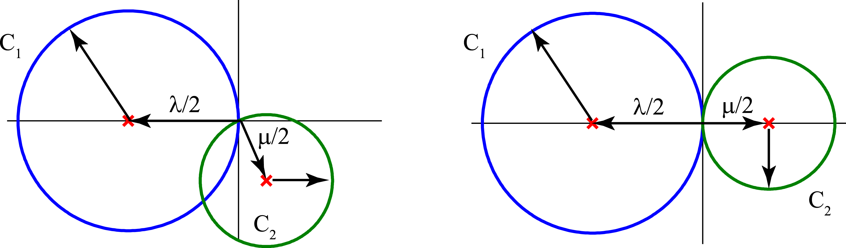
Figure 1. The solutions of the system (3.5) occur at the intersections of the circles
 $C_{1}$
(blue) and
$C_{1}$
(blue) and
 $C_{2}$
(green).
$C_{2}$
(green).
 $C_{1}$
has centre
$C_{1}$
has centre
 $\unicode[STIX]{x1D740}/2$
and radius
$\unicode[STIX]{x1D740}/2$
and radius
 $|\unicode[STIX]{x1D740}/2|$
.
$|\unicode[STIX]{x1D740}/2|$
.
 $C_{2}$
has centre
$C_{2}$
has centre
 $\unicode[STIX]{x1D741}/2$
and radius
$\unicode[STIX]{x1D741}/2$
and radius
 $|\unicode[STIX]{x1D741}/2|$
. In the cases shown here
$|\unicode[STIX]{x1D741}/2|$
. In the cases shown here
 $|\unicode[STIX]{x1D740}|\neq |\unicode[STIX]{x1D741}|$
. In the graph on the right-hand side
$|\unicode[STIX]{x1D740}|\neq |\unicode[STIX]{x1D741}|$
. In the graph on the right-hand side
 $\unicode[STIX]{x1D740}$
and
$\unicode[STIX]{x1D740}$
and
 $\unicode[STIX]{x1D741}$
are anti-parallel and the system has only the trivial solution; in the graph on the left-hand side
$\unicode[STIX]{x1D741}$
are anti-parallel and the system has only the trivial solution; in the graph on the left-hand side
 $\unicode[STIX]{x1D740}$
and
$\unicode[STIX]{x1D740}$
and
 $\unicode[STIX]{x1D741}$
are linearly independent and there is a unique non-trivial solution.
$\unicode[STIX]{x1D741}$
are linearly independent and there is a unique non-trivial solution.
For an ideal MHD shock with the property that the coplanarity theorem holds, the system (3.5) is degenerate, that is,
 $\unicode[STIX]{x1D740}=\unicode[STIX]{x1D741}$
. To show this it is sufficient to show
$\unicode[STIX]{x1D740}=\unicode[STIX]{x1D741}$
. To show this it is sufficient to show
 $u=s$
and
$u=s$
and
 $v=t$
in the special case where
$v=t$
in the special case where
 $\hat{\boldsymbol{\unicode[STIX]{x1D702}}}$
is the true shock normal,
$\hat{\boldsymbol{\unicode[STIX]{x1D702}}}$
is the true shock normal,
 $\hat{\boldsymbol{\unicode[STIX]{x1D702}}}=\hat{\boldsymbol{n}}$
, and
$\hat{\boldsymbol{\unicode[STIX]{x1D702}}}=\hat{\boldsymbol{n}}$
, and
 $\hat{\unicode[STIX]{x1D743}}$
is orthogonal to both
$\hat{\unicode[STIX]{x1D743}}$
is orthogonal to both
 $\unicode[STIX]{x0394}\boldsymbol{B}$
and
$\unicode[STIX]{x0394}\boldsymbol{B}$
and
 $\hat{\boldsymbol{n}}$
. It is sufficient to consider this special case since for any other admissible choice of the unit vector
$\hat{\boldsymbol{n}}$
. It is sufficient to consider this special case since for any other admissible choice of the unit vector
 $\hat{\boldsymbol{\unicode[STIX]{x1D702}}}$
, say
$\hat{\boldsymbol{\unicode[STIX]{x1D702}}}$
, say
 $\hat{\boldsymbol{\unicode[STIX]{x1D702}}}^{\prime }$
, the corresponding unit vectors
$\hat{\boldsymbol{\unicode[STIX]{x1D702}}}^{\prime }$
, the corresponding unit vectors
 $\hat{\boldsymbol{\unicode[STIX]{x1D702}}}^{\prime }$
and
$\hat{\boldsymbol{\unicode[STIX]{x1D702}}}^{\prime }$
and
 $\hat{\unicode[STIX]{x1D743}}^{\prime }$
are each expressible as a linear superposition of the vectors
$\hat{\unicode[STIX]{x1D743}}^{\prime }$
are each expressible as a linear superposition of the vectors
 $\hat{\boldsymbol{\unicode[STIX]{x1D702}}}$
and
$\hat{\boldsymbol{\unicode[STIX]{x1D702}}}$
and
 $\hat{\unicode[STIX]{x1D743}}$
in the special case where
$\hat{\unicode[STIX]{x1D743}}$
in the special case where
 $\hat{\boldsymbol{\unicode[STIX]{x1D702}}}=\hat{\boldsymbol{n}}$
and
$\hat{\boldsymbol{\unicode[STIX]{x1D702}}}=\hat{\boldsymbol{n}}$
and
 $\hat{\unicode[STIX]{x1D743}}\propto \unicode[STIX]{x0394}\boldsymbol{B}\times \hat{\boldsymbol{n}}$
. In this special case it follows from (3.1) that
$\hat{\unicode[STIX]{x1D743}}\propto \unicode[STIX]{x0394}\boldsymbol{B}\times \hat{\boldsymbol{n}}$
. In this special case it follows from (3.1) that
 $(x,y)=(V_{\text{sh}},0)$
and, therefore, setting
$(x,y)=(V_{\text{sh}},0)$
and, therefore, setting
 $y=0$
in (3.2) and (3.3) shows that
$y=0$
in (3.2) and (3.3) shows that
 $u=s$
. The condition
$u=s$
. The condition
 $v=t$
may be written
$v=t$
may be written
 $$\begin{eqnarray}\left[\frac{\unicode[STIX]{x1D70C}_{1}\boldsymbol{V}_{1}+\unicode[STIX]{x1D70C}_{2}\boldsymbol{V}_{2}}{\unicode[STIX]{x1D70C}_{1}+\unicode[STIX]{x1D70C}_{2}}-\frac{|\unicode[STIX]{x0394}\boldsymbol{V}|^{2}}{\unicode[STIX]{x0394}\boldsymbol{V}\boldsymbol{\cdot }\unicode[STIX]{x0394}(\boldsymbol{B}/\unicode[STIX]{x1D70C})}\left(\frac{\boldsymbol{B}_{1}+\boldsymbol{B}_{2}}{\unicode[STIX]{x1D70C}_{1}+\unicode[STIX]{x1D70C}_{2}}\right)\right]\boldsymbol{\cdot }\hat{\unicode[STIX]{x1D743}}=\frac{(\unicode[STIX]{x1D70C}_{1}\boldsymbol{V}_{1}-\unicode[STIX]{x1D70C}_{2}\boldsymbol{V}_{2})}{\unicode[STIX]{x1D70C}_{1}-\unicode[STIX]{x1D70C}_{2}}\boldsymbol{\cdot }\hat{\unicode[STIX]{x1D743}}\end{eqnarray}$$
or, equivalently,
 $$\begin{eqnarray}\left[\frac{2\unicode[STIX]{x1D70C}_{1}\unicode[STIX]{x1D70C}_{2}}{\unicode[STIX]{x1D70C}_{1}^{2}-\unicode[STIX]{x1D70C}_{2}^{2}}\unicode[STIX]{x0394}\boldsymbol{V}+\frac{|\unicode[STIX]{x0394}\boldsymbol{V}|^{2}}{\unicode[STIX]{x0394}\boldsymbol{V}\boldsymbol{\cdot }\unicode[STIX]{x0394}(\boldsymbol{B}/\unicode[STIX]{x1D70C})}\left(\frac{\boldsymbol{B}_{1}+\boldsymbol{B}_{2}}{\unicode[STIX]{x1D70C}_{1}+\unicode[STIX]{x1D70C}_{2}}\right)\right]\boldsymbol{\cdot }\hat{\unicode[STIX]{x1D743}}=0.\end{eqnarray}$$
When the coplanarity theorem holds the tangential components of
 $\boldsymbol{B}_{1}$
,
$\boldsymbol{B}_{1}$
,
 $\boldsymbol{B}_{2}$
and
$\boldsymbol{B}_{2}$
and
 $\unicode[STIX]{x0394}\boldsymbol{V}$
are each colinear with the vector
$\unicode[STIX]{x0394}\boldsymbol{V}$
are each colinear with the vector
 $\unicode[STIX]{x0394}\boldsymbol{B}$
(Landau & Lifshitz Reference Landau and Lifshitz1960; Colburn & Sonett Reference Colburn and Sonett1966) and, therefore, in the special case where
$\unicode[STIX]{x0394}\boldsymbol{B}$
(Landau & Lifshitz Reference Landau and Lifshitz1960; Colburn & Sonett Reference Colburn and Sonett1966) and, therefore, in the special case where
 $\hat{\boldsymbol{\unicode[STIX]{x1D702}}}=\hat{\boldsymbol{n}}$
and
$\hat{\boldsymbol{\unicode[STIX]{x1D702}}}=\hat{\boldsymbol{n}}$
and
 $\hat{\unicode[STIX]{x1D743}}\propto \unicode[STIX]{x0394}\boldsymbol{B}\times \hat{\boldsymbol{n}}$
, each of the vectors in the rectangular bracket in (3.10) is orthogonal to
$\hat{\unicode[STIX]{x1D743}}\propto \unicode[STIX]{x0394}\boldsymbol{B}\times \hat{\boldsymbol{n}}$
, each of the vectors in the rectangular bracket in (3.10) is orthogonal to
 $\hat{\unicode[STIX]{x1D743}}$
since
$\hat{\unicode[STIX]{x1D743}}$
since
 $\hat{\unicode[STIX]{x1D743}}$
is orthogonal to both
$\hat{\unicode[STIX]{x1D743}}$
is orthogonal to both
 $\unicode[STIX]{x0394}\boldsymbol{B}$
and
$\unicode[STIX]{x0394}\boldsymbol{B}$
and
 $\hat{\boldsymbol{n}}$
. This completes the proof.
$\hat{\boldsymbol{n}}$
. This completes the proof.
Thus, when the coplanarity theorem holds the system of three scalar equations (2.1), (2.2) and (2.8) are degenerate and an uncountably infinite number of non-trivial solutions exists. For an ideal MHD shock, the coplanarity theorem holds when the pressure tensor is isotropic, for example, or when the pressure tensor is gyrotropic with respect to the direction of the magnetic field vector
 $\boldsymbol{B}$
(Hudson Reference Hudson1970).
$\boldsymbol{B}$
(Hudson Reference Hudson1970).
4 Tangential flux of linear momentum
In the search for a minimal system of equations that uniquely determine the shock velocity it is logical to next consider the jump condition for the linear momentum flux. In the case of a scalar pressure, the jump condition for the flux of linear momentum is
 $$\begin{eqnarray}\left[\!\!\left[\unicode[STIX]{x1D70C}\boldsymbol{V}^{\prime }V_{n}^{\prime }+\left(p+\frac{B^{2}}{2\unicode[STIX]{x1D707}_{0}}\right)\hat{\boldsymbol{n}}-\frac{\boldsymbol{B}B_{n}}{\unicode[STIX]{x1D707}_{0}}\right]\!\!\right]=0,\end{eqnarray}$$
where
 $\boldsymbol{V}^{\prime }=\boldsymbol{V}-\boldsymbol{V}_{\text{sh}}$
,
$\boldsymbol{V}^{\prime }=\boldsymbol{V}-\boldsymbol{V}_{\text{sh}}$
,
 $V_{n}^{\prime }=\boldsymbol{V}^{\prime }\boldsymbol{\cdot }\hat{\boldsymbol{n}}$
,
$V_{n}^{\prime }=\boldsymbol{V}^{\prime }\boldsymbol{\cdot }\hat{\boldsymbol{n}}$
,
 $B_{n}=\boldsymbol{B}\boldsymbol{\cdot }\hat{\boldsymbol{n}}$
and the double brackets denote the change across the discontinuity, that is,
$B_{n}=\boldsymbol{B}\boldsymbol{\cdot }\hat{\boldsymbol{n}}$
and the double brackets denote the change across the discontinuity, that is,
 $\unicode[STIX]{x27E6}Q\unicode[STIX]{x27E7}\equiv Q_{1}-Q_{2}$
. The normal and tangential components of the jump condition (4.1) may be written
$\unicode[STIX]{x27E6}Q\unicode[STIX]{x27E7}\equiv Q_{1}-Q_{2}$
. The normal and tangential components of the jump condition (4.1) may be written
 $$\begin{eqnarray}\left[\!\!\left[\unicode[STIX]{x1D70C}V_{n}^{\prime 2}+p+\frac{B^{2}}{2\unicode[STIX]{x1D707}_{0}}\right]\!\!\right]=0\end{eqnarray}$$
and
 $$\begin{eqnarray}\left[\!\!\left[(\unicode[STIX]{x1D70C}V_{n}^{\prime })\boldsymbol{V}^{\prime }\times \hat{\boldsymbol{n}}-\frac{B_{n}}{\unicode[STIX]{x1D707}_{0}}\boldsymbol{B}\times \hat{\boldsymbol{n}}\right]\!\!\right]=0,\end{eqnarray}$$
respectively. Thus, when the pressure tensor is isotropic the jump condition (4.3) is independent of the pressure and, consequently, in this case there are four and only four jump conditions that are independent of the pressure (including the three discussed in § 2). Since
 $\unicode[STIX]{x1D70C}V_{n}^{\prime }$
and
$\unicode[STIX]{x1D70C}V_{n}^{\prime }$
and
 $B_{n}$
are both continuous, the jump condition (4.3) implies
$B_{n}$
are both continuous, the jump condition (4.3) implies
 $$\begin{eqnarray}(\unicode[STIX]{x1D70C}_{1}V_{1n}^{\prime })(\unicode[STIX]{x0394}\boldsymbol{V}\times \hat{\boldsymbol{n}})=\frac{B_{1n}}{\unicode[STIX]{x1D707}_{0}}(\unicode[STIX]{x0394}\boldsymbol{B}\times \hat{\boldsymbol{n}})\end{eqnarray}$$
or, taking the cross-product of this equation with
 $\hat{\boldsymbol{n}}$
and using the fact that
$\hat{\boldsymbol{n}}$
and using the fact that
 $\unicode[STIX]{x0394}\boldsymbol{B}\boldsymbol{\cdot }\hat{\boldsymbol{n}}=0$
,
$\unicode[STIX]{x0394}\boldsymbol{B}\boldsymbol{\cdot }\hat{\boldsymbol{n}}=0$
,
 $$\begin{eqnarray}(\unicode[STIX]{x1D70C}_{1}V_{1n}^{\prime })[\unicode[STIX]{x0394}\boldsymbol{V}-(\unicode[STIX]{x0394}\boldsymbol{V}\boldsymbol{\cdot }\hat{\boldsymbol{n}})\hat{\boldsymbol{n}}]=\frac{B_{1n}}{\unicode[STIX]{x1D707}_{0}}\unicode[STIX]{x0394}\boldsymbol{B}.\end{eqnarray}$$
For non-perpendicular shocks
 $\unicode[STIX]{x1D70C}V_{n}^{\prime }\neq 0$
and
$\unicode[STIX]{x1D70C}V_{n}^{\prime }\neq 0$
and
 $B_{n}\neq 0$
and, therefore, it follows from (4.5) that the tangential component of
$B_{n}\neq 0$
and, therefore, it follows from (4.5) that the tangential component of
 $\unicode[STIX]{x0394}\boldsymbol{V}$
is proportional to
$\unicode[STIX]{x0394}\boldsymbol{V}$
is proportional to
 $\unicode[STIX]{x0394}\boldsymbol{B}$
. By virtue of the vector relation (4.5) the jump condition for the tangential momentum flux (4.3) reduces to the scalar equation
$\unicode[STIX]{x0394}\boldsymbol{B}$
. By virtue of the vector relation (4.5) the jump condition for the tangential momentum flux (4.3) reduces to the scalar equation
 $$\begin{eqnarray}(\unicode[STIX]{x1D70C}_{1}V_{1n}^{\prime })(\unicode[STIX]{x0394}\boldsymbol{V}\boldsymbol{\cdot }\unicode[STIX]{x0394}\boldsymbol{B})=\frac{B_{1n}}{\unicode[STIX]{x1D707}_{0}}|\unicode[STIX]{x0394}\boldsymbol{B}|^{2}.\end{eqnarray}$$
An equivalent form that is symmetric under interchange of the indices 1 and 2 is
 $$\begin{eqnarray}(\unicode[STIX]{x1D70C}_{1}V_{1n}^{\prime }+\unicode[STIX]{x1D70C}_{2}V_{2n}^{\prime })(\unicode[STIX]{x0394}\boldsymbol{V}\boldsymbol{\cdot }\unicode[STIX]{x0394}\boldsymbol{B})=\left(\frac{B_{1n}+B_{2n}}{\unicode[STIX]{x1D707}_{0}}\right)|\unicode[STIX]{x0394}\boldsymbol{B}|^{2}.\end{eqnarray}$$
Equations (4.6) and (4.7) yield the following expressions for the shock speed:
 $$\begin{eqnarray}\displaystyle V_{\text{sh}} & = & \displaystyle \left[\boldsymbol{V}_{1}-\frac{|\unicode[STIX]{x0394}\boldsymbol{B}|^{2}}{\unicode[STIX]{x1D707}_{0}\unicode[STIX]{x0394}\boldsymbol{V}\boldsymbol{\cdot }\unicode[STIX]{x0394}\boldsymbol{B}}\left(\frac{\boldsymbol{B}_{1}}{\unicode[STIX]{x1D70C}_{1}}\right)\right]\boldsymbol{\cdot }\hat{\boldsymbol{n}}\end{eqnarray}$$
 $$\begin{eqnarray}\displaystyle & = & \displaystyle \left[\boldsymbol{V}_{2}-\frac{|\unicode[STIX]{x0394}\boldsymbol{B}|^{2}}{\unicode[STIX]{x1D707}_{0}\unicode[STIX]{x0394}\boldsymbol{V}\boldsymbol{\cdot }\unicode[STIX]{x0394}\boldsymbol{B}}\left(\frac{\boldsymbol{B}_{2}}{\unicode[STIX]{x1D70C}_{2}}\right)\right]\boldsymbol{\cdot }\hat{\boldsymbol{n}}\end{eqnarray}$$
 $$\begin{eqnarray}\displaystyle & = & \displaystyle \left[\frac{\unicode[STIX]{x1D70C}_{1}\boldsymbol{V}_{1}+\unicode[STIX]{x1D70C}_{2}\boldsymbol{V}_{2}}{\unicode[STIX]{x1D70C}_{1}+\unicode[STIX]{x1D70C}_{2}}-\frac{|\unicode[STIX]{x0394}\boldsymbol{B}|^{2}}{\unicode[STIX]{x1D707}_{0}\unicode[STIX]{x0394}\boldsymbol{V}\boldsymbol{\cdot }\unicode[STIX]{x0394}\boldsymbol{B}}\left(\frac{\boldsymbol{B}_{1}+\boldsymbol{B}_{2}}{\unicode[STIX]{x1D70C}_{1}+\unicode[STIX]{x1D70C}_{2}}\right)\right]\boldsymbol{\cdot }\hat{\boldsymbol{n}},\end{eqnarray}$$
etc. Making the substitution (3.1), the scalar equation (4.10) takes the simple and familiar form
 $\boldsymbol{x}\boldsymbol{\cdot }(\boldsymbol{x}-\hat{\unicode[STIX]{x1D741}}^{\prime })=0$
, where
$\boldsymbol{x}\boldsymbol{\cdot }(\boldsymbol{x}-\hat{\unicode[STIX]{x1D741}}^{\prime })=0$
, where
 $\hat{\unicode[STIX]{x1D741}}^{\prime }=(s^{\prime },t^{\prime })$
,
$\hat{\unicode[STIX]{x1D741}}^{\prime }=(s^{\prime },t^{\prime })$
,
 $$\begin{eqnarray}s^{\prime }=\left[\frac{\unicode[STIX]{x1D70C}_{1}\boldsymbol{V}_{1}+\unicode[STIX]{x1D70C}_{2}\boldsymbol{V}_{2}}{\unicode[STIX]{x1D70C}_{1}+\unicode[STIX]{x1D70C}_{2}}-\frac{|\unicode[STIX]{x0394}\boldsymbol{B}|^{2}}{\unicode[STIX]{x1D707}_{0}\unicode[STIX]{x0394}\boldsymbol{V}\boldsymbol{\cdot }\unicode[STIX]{x0394}\boldsymbol{B}}\left(\frac{\boldsymbol{B}_{1}+\boldsymbol{B}_{2}}{\unicode[STIX]{x1D70C}_{1}+\unicode[STIX]{x1D70C}_{2}}\right)\right]\boldsymbol{\cdot }\hat{\boldsymbol{\unicode[STIX]{x1D702}}},\end{eqnarray}$$
and
 $$\begin{eqnarray}t^{\prime }=\left[\frac{\unicode[STIX]{x1D70C}_{1}\boldsymbol{V}_{1}+\unicode[STIX]{x1D70C}_{2}\boldsymbol{V}_{2}}{\unicode[STIX]{x1D70C}_{1}+\unicode[STIX]{x1D70C}_{2}}-\frac{|\unicode[STIX]{x0394}\boldsymbol{B}|^{2}}{\unicode[STIX]{x1D707}_{0}\unicode[STIX]{x0394}\boldsymbol{V}\boldsymbol{\cdot }\unicode[STIX]{x0394}\boldsymbol{B}}\left(\frac{\boldsymbol{B}_{1}+\boldsymbol{B}_{2}}{\unicode[STIX]{x1D70C}_{1}+\unicode[STIX]{x1D70C}_{2}}\right)\right]\boldsymbol{\cdot }\hat{\unicode[STIX]{x1D743}}.\end{eqnarray}$$
It is easy to see that this is identical to the scalar equation
 $\boldsymbol{x}\boldsymbol{\cdot }(\boldsymbol{x}-\hat{\unicode[STIX]{x1D741}})=0$
derived in § 3 since
$\boldsymbol{x}\boldsymbol{\cdot }(\boldsymbol{x}-\hat{\unicode[STIX]{x1D741}})=0$
derived in § 3 since
 $\hat{\unicode[STIX]{x1D741}}^{\prime }=\hat{\unicode[STIX]{x1D741}}$
or, equivalently,
$\hat{\unicode[STIX]{x1D741}}^{\prime }=\hat{\unicode[STIX]{x1D741}}$
or, equivalently,
 $s^{\prime }=s$
and
$s^{\prime }=s$
and
 $t^{\prime }=t$
; this identity is a simple consequence of the relations (2.7) and (4.6) which together imply
$t^{\prime }=t$
; this identity is a simple consequence of the relations (2.7) and (4.6) which together imply
 $$\begin{eqnarray}\frac{|\unicode[STIX]{x0394}\boldsymbol{V}|^{2}}{\unicode[STIX]{x0394}\boldsymbol{V}\boldsymbol{\cdot }\unicode[STIX]{x0394}(\boldsymbol{B}/\unicode[STIX]{x1D70C})}=\frac{\unicode[STIX]{x1D70C}_{1}V_{1n}^{\prime }}{B_{1n}}=\frac{|\unicode[STIX]{x0394}\boldsymbol{B}|^{2}}{\unicode[STIX]{x1D707}_{0}\unicode[STIX]{x0394}\boldsymbol{V}\boldsymbol{\cdot }\unicode[STIX]{x0394}\boldsymbol{B}}.\end{eqnarray}$$
Hence, the jump condition for the tangential flux of linear momentum (4.3) reduces to a scalar equation for
 $\boldsymbol{V}_{\text{sh}}$
that is equivalent to the two degenerate equations derived in § 3. It does, however, provide a new vector relation (4.5) between the states upstream and downstream that can be useful when fitting experimental data.
$\boldsymbol{V}_{\text{sh}}$
that is equivalent to the two degenerate equations derived in § 3. It does, however, provide a new vector relation (4.5) between the states upstream and downstream that can be useful when fitting experimental data.
5 Normal flux of linear momentum
In the case of an isotropic pressure tensor, in order to obtain three non-degenerate scalar equations that yield a unique non-trivial solution for the shock velocity it is not enough to use solely those jump relations that are independent of the pressure. It shall now be shown that the jump condition for the normal component of the linear momentum flux (4.2), when combined with the three jump conditions considered in § 2, is sufficient to uniquely determine
 $\boldsymbol{V}_{\text{sh}}$
. The jump condition (4.2) may be written
$\boldsymbol{V}_{\text{sh}}$
. The jump condition (4.2) may be written
 $$\begin{eqnarray}\unicode[STIX]{x1D70C}_{1}[(\boldsymbol{V}_{1}-\boldsymbol{V}_{\text{sh}})\boldsymbol{\cdot }\boldsymbol{V}_{\text{sh}}]^{2}-\unicode[STIX]{x1D70C}_{2}[(\boldsymbol{V}_{2}-\boldsymbol{V}_{\text{sh}})\boldsymbol{\cdot }\boldsymbol{V}_{\text{sh}}]^{2}=-\unicode[STIX]{x0394}\left(p+\frac{B^{2}}{2\unicode[STIX]{x1D707}_{0}}\right)\boldsymbol{V}_{\text{sh}}\boldsymbol{\cdot }\boldsymbol{V}_{\text{sh}},\end{eqnarray}$$
where
 $$\begin{eqnarray}\unicode[STIX]{x0394}\left(p+\frac{B^{2}}{2\unicode[STIX]{x1D707}_{0}}\right)=(p_{1}-p_{2})+\frac{B_{1}^{2}-B_{2}^{2}}{2\unicode[STIX]{x1D707}_{0}}\end{eqnarray}$$
and
 $B^{2}=\boldsymbol{B}\boldsymbol{\cdot }\boldsymbol{B}$
. The left-hand side of (5.1) is
$B^{2}=\boldsymbol{B}\boldsymbol{\cdot }\boldsymbol{B}$
. The left-hand side of (5.1) is
 $$\begin{eqnarray}[\sqrt{\unicode[STIX]{x1D70C}_{1}}(\boldsymbol{V}_{1}-\boldsymbol{V}_{\text{sh}})\boldsymbol{\cdot }\boldsymbol{V}_{\text{sh}}+\sqrt{\unicode[STIX]{x1D70C}_{2}}(\boldsymbol{V}_{2}-\boldsymbol{V}_{\text{sh}})\boldsymbol{\cdot }\boldsymbol{V}_{\text{sh}}][\sqrt{\unicode[STIX]{x1D70C}_{1}}(\boldsymbol{V}_{1}-\boldsymbol{V}_{\text{sh}})\boldsymbol{\cdot }\boldsymbol{V}_{\text{sh}}-\sqrt{\unicode[STIX]{x1D70C}_{2}}(\boldsymbol{V}_{2}-\boldsymbol{V}_{\text{sh}})\boldsymbol{\cdot }\boldsymbol{V}_{\text{sh}}]\end{eqnarray}$$
or, equivalently,
 $$\begin{eqnarray}\displaystyle & & \displaystyle \{[(\sqrt{\unicode[STIX]{x1D70C}_{1}}\boldsymbol{V}_{1}+\sqrt{\unicode[STIX]{x1D70C}_{2}}\boldsymbol{V}_{2})-(\sqrt{\unicode[STIX]{x1D70C}_{1}}+\sqrt{\unicode[STIX]{x1D70C}_{2}})\boldsymbol{V}_{\text{sh}})]\boldsymbol{\cdot }\boldsymbol{V}_{\text{sh}}\}\nonumber\\ \displaystyle & & \displaystyle \quad \times \,\{[(\sqrt{\unicode[STIX]{x1D70C}_{1}}\boldsymbol{V}_{1}-\sqrt{\unicode[STIX]{x1D70C}_{2}}\boldsymbol{V}_{2})-(\sqrt{\unicode[STIX]{x1D70C}_{1}}-\sqrt{\unicode[STIX]{x1D70C}_{2}})\boldsymbol{V}_{\text{sh}})]\boldsymbol{\cdot }\boldsymbol{V}_{\text{sh}}\}.\end{eqnarray}$$
Thus, using the representation (3.1), equation (5.1) takes the form
 $$\begin{eqnarray}[(\boldsymbol{x}-\boldsymbol{a})\boldsymbol{\cdot }\boldsymbol{x}][(\boldsymbol{x}-\boldsymbol{b})\boldsymbol{\cdot }\boldsymbol{x}]=-\frac{1}{\unicode[STIX]{x1D70C}_{1}-\unicode[STIX]{x1D70C}_{2}}\unicode[STIX]{x0394}\left(p+\frac{B^{2}}{2\unicode[STIX]{x1D707}_{0}}\right)(\boldsymbol{x}\boldsymbol{\cdot }\boldsymbol{x}),\end{eqnarray}$$
where
 $$\begin{eqnarray}\displaystyle & \displaystyle \boldsymbol{a}=\left(\frac{\sqrt{\unicode[STIX]{x1D70C}_{1}}\boldsymbol{V}_{1}+\sqrt{\unicode[STIX]{x1D70C}_{2}}\boldsymbol{V}_{2}}{\sqrt{\unicode[STIX]{x1D70C}_{1}}+\sqrt{\unicode[STIX]{x1D70C}_{2}}}\boldsymbol{\cdot }\hat{\boldsymbol{\unicode[STIX]{x1D702}}},~\frac{\sqrt{\unicode[STIX]{x1D70C}_{1}}\boldsymbol{V}_{1}+\sqrt{\unicode[STIX]{x1D70C}_{2}}\boldsymbol{V}_{2}}{\sqrt{\unicode[STIX]{x1D70C}_{1}}+\sqrt{\unicode[STIX]{x1D70C}_{2}}}\boldsymbol{\cdot }\hat{\unicode[STIX]{x1D743}}\right), & \displaystyle\end{eqnarray}$$
 $$\begin{eqnarray}\displaystyle & \displaystyle \boldsymbol{b}=\left(\frac{\sqrt{\unicode[STIX]{x1D70C}_{1}}\boldsymbol{V}_{1}-\sqrt{\unicode[STIX]{x1D70C}_{2}}\boldsymbol{V}_{2}}{\sqrt{\unicode[STIX]{x1D70C}_{1}}-\sqrt{\unicode[STIX]{x1D70C}_{2}}}\boldsymbol{\cdot }\hat{\boldsymbol{\unicode[STIX]{x1D702}}},~\frac{\sqrt{\unicode[STIX]{x1D70C}_{1}}\boldsymbol{V}_{1}-\sqrt{\unicode[STIX]{x1D70C}_{2}}\boldsymbol{V}_{2}}{\sqrt{\unicode[STIX]{x1D70C}_{1}}-\sqrt{\unicode[STIX]{x1D70C}_{2}}}\boldsymbol{\cdot }\hat{\unicode[STIX]{x1D743}}\right), & \displaystyle\end{eqnarray}$$
and, as in § 3,
 $\boldsymbol{x}=(x,y)$
.
$\boldsymbol{x}=(x,y)$
.
Three of the four scalar equations derived from the jump conditions (2.1), (2.2), (2.3) and (4.3) were previously shown to be degenerate. The general solution of those four scalar equations derived in § 3 is
 $\boldsymbol{x}=(\unicode[STIX]{x1D740}+|\unicode[STIX]{x1D740}|\hat{\boldsymbol{u}})/2$
, where
$\boldsymbol{x}=(\unicode[STIX]{x1D740}+|\unicode[STIX]{x1D740}|\hat{\boldsymbol{u}})/2$
, where
 $\unicode[STIX]{x1D740}$
is defined by (3.6) and
$\unicode[STIX]{x1D740}$
is defined by (3.6) and
 $\hat{\boldsymbol{u}}=(\cos \unicode[STIX]{x1D703},\sin \unicode[STIX]{x1D703})$
is any arbitrary unit vector. To simultaneously solve the scalar equation (5.5) together with the four previous equations substitute
$\hat{\boldsymbol{u}}=(\cos \unicode[STIX]{x1D703},\sin \unicode[STIX]{x1D703})$
is any arbitrary unit vector. To simultaneously solve the scalar equation (5.5) together with the four previous equations substitute
 $\boldsymbol{x}=(\unicode[STIX]{x1D740}+|\unicode[STIX]{x1D740}|\hat{\boldsymbol{u}})/2$
into (5.5) to obtain
$\boldsymbol{x}=(\unicode[STIX]{x1D740}+|\unicode[STIX]{x1D740}|\hat{\boldsymbol{u}})/2$
into (5.5) to obtain
 $$\begin{eqnarray}(\boldsymbol{P}\boldsymbol{\cdot }\hat{\boldsymbol{u}}+L)(\boldsymbol{Q}\boldsymbol{\cdot }\hat{\boldsymbol{u}}+M)+(\boldsymbol{R}\boldsymbol{\cdot }\hat{\boldsymbol{u}}+N)=0,\end{eqnarray}$$
where
 $$\begin{eqnarray}\boldsymbol{P}=\frac{1}{2}|\unicode[STIX]{x1D740}|(\unicode[STIX]{x1D740}-\boldsymbol{a}),\quad \boldsymbol{Q}=\frac{1}{2}|\unicode[STIX]{x1D740}|(\unicode[STIX]{x1D740}-\boldsymbol{b}),\quad \boldsymbol{R}=\frac{|\unicode[STIX]{x1D740}|\unicode[STIX]{x1D740}}{2(\unicode[STIX]{x1D70C}_{1}-\unicode[STIX]{x1D70C}_{2})}\unicode[STIX]{x0394}\left(p+\frac{B^{2}}{2\unicode[STIX]{x1D707}_{0}}\right),\end{eqnarray}$$
 $$\begin{eqnarray}L=\frac{1}{2}\unicode[STIX]{x1D740}\boldsymbol{\cdot }(\unicode[STIX]{x1D740}-\boldsymbol{a}),\quad M=\frac{1}{2}\unicode[STIX]{x1D740}\boldsymbol{\cdot }(\unicode[STIX]{x1D740}-\boldsymbol{b}),\quad N=\frac{\unicode[STIX]{x1D706}^{2}}{2(\unicode[STIX]{x1D70C}_{1}-\unicode[STIX]{x1D70C}_{2})}\unicode[STIX]{x0394}\left(p+\frac{B^{2}}{2\unicode[STIX]{x1D707}_{0}}\right),\end{eqnarray}$$
and
 $\unicode[STIX]{x1D706}^{2}=\unicode[STIX]{x1D740}\boldsymbol{\cdot }\unicode[STIX]{x1D740}$
. Using the definitions (3.6) and (5.6) it is easy to show that
$\unicode[STIX]{x1D706}^{2}=\unicode[STIX]{x1D740}\boldsymbol{\cdot }\unicode[STIX]{x1D740}$
. Using the definitions (3.6) and (5.6) it is easy to show that
 $$\begin{eqnarray}\unicode[STIX]{x1D740}-\boldsymbol{a}=-(\unicode[STIX]{x1D740}-\boldsymbol{b})=\frac{\sqrt{\unicode[STIX]{x1D70C}_{1}\unicode[STIX]{x1D70C}_{2}}}{\unicode[STIX]{x1D70C}_{1}-\unicode[STIX]{x1D70C}_{2}}(\unicode[STIX]{x0394}\boldsymbol{V}\boldsymbol{\cdot }\hat{\boldsymbol{\unicode[STIX]{x1D702}}},\unicode[STIX]{x0394}\boldsymbol{V}\boldsymbol{\cdot }\hat{\unicode[STIX]{x1D743}})\end{eqnarray}$$
and, therefore,
 $$\begin{eqnarray}\displaystyle \boldsymbol{P}\boldsymbol{\cdot }\hat{\boldsymbol{u}}+L & = & \displaystyle -(\boldsymbol{Q}\boldsymbol{\cdot }\hat{\boldsymbol{u}}+M)\nonumber\\ \displaystyle & = & \displaystyle \frac{1}{2}|\unicode[STIX]{x1D740}||\unicode[STIX]{x0394}V_{n}|\frac{\sqrt{\unicode[STIX]{x1D70C}_{1}\unicode[STIX]{x1D70C}_{2}}}{\unicode[STIX]{x1D70C}_{1}-\unicode[STIX]{x1D70C}_{2}}\left[\frac{\unicode[STIX]{x0394}\boldsymbol{V}\boldsymbol{\cdot }\hat{\boldsymbol{\unicode[STIX]{x1D702}}}}{|\unicode[STIX]{x0394}V_{n}|}\left(\frac{u}{\sqrt{u^{2}+v^{2}}}+\cos \unicode[STIX]{x1D703}\right)\right.\nonumber\\ \displaystyle & & \displaystyle \left.+\,\frac{\unicode[STIX]{x0394}\boldsymbol{V}\boldsymbol{\cdot }\hat{\unicode[STIX]{x1D743}}}{|\unicode[STIX]{x0394}V_{n}|}\left(\frac{v}{\sqrt{u^{2}+v^{2}}}+\sin \unicode[STIX]{x1D703}\right)\right]\end{eqnarray}$$
or, equivalently,
 $$\begin{eqnarray}\displaystyle & & \displaystyle \frac{1}{2}|\unicode[STIX]{x1D740}||\unicode[STIX]{x0394}V_{n}|\frac{\sqrt{\unicode[STIX]{x1D70C}_{1}\unicode[STIX]{x1D70C}_{2}}}{\unicode[STIX]{x1D70C}_{1}-\unicode[STIX]{x1D70C}_{2}}[\cos \unicode[STIX]{x1D719}(\cos \unicode[STIX]{x1D703}_{\unicode[STIX]{x1D706}}+\cos \unicode[STIX]{x1D703})+\sin \unicode[STIX]{x1D719}(\sin \unicode[STIX]{x1D703}_{\unicode[STIX]{x1D706}}+\sin \unicode[STIX]{x1D703})]\nonumber\\ \displaystyle & & \displaystyle \quad =\frac{1}{2}|\unicode[STIX]{x1D740}||\unicode[STIX]{x0394}V_{n}|\frac{\sqrt{\unicode[STIX]{x1D70C}_{1}\unicode[STIX]{x1D70C}_{2}}}{\unicode[STIX]{x1D70C}_{1}-\unicode[STIX]{x1D70C}_{2}}[\cos (\unicode[STIX]{x1D703}_{\unicode[STIX]{x1D706}}-\unicode[STIX]{x1D719})+\cos (\unicode[STIX]{x1D703}-\unicode[STIX]{x1D719})],\end{eqnarray}$$
where the angle
 $\unicode[STIX]{x1D703}_{\unicode[STIX]{x1D706}}$
is defined by
$\unicode[STIX]{x1D703}_{\unicode[STIX]{x1D706}}$
is defined by
 $$\begin{eqnarray}\cos (\unicode[STIX]{x1D703}_{\unicode[STIX]{x1D706}})=\frac{u}{\sqrt{u^{2}+v^{2}}},\quad \sin (\unicode[STIX]{x1D703}_{\unicode[STIX]{x1D706}})=\frac{v}{\sqrt{u^{2}+v^{2}}},\end{eqnarray}$$
and the angle
 $\unicode[STIX]{x1D719}$
is defined by
$\unicode[STIX]{x1D719}$
is defined by
 $$\begin{eqnarray}\cos (\unicode[STIX]{x1D719})=\frac{\unicode[STIX]{x0394}\boldsymbol{V}\boldsymbol{\cdot }\hat{\boldsymbol{\unicode[STIX]{x1D702}}}}{|\unicode[STIX]{x0394}V_{n}|},\quad \sin (\unicode[STIX]{x1D719})=\frac{\unicode[STIX]{x0394}\boldsymbol{V}\boldsymbol{\cdot }\hat{\unicode[STIX]{x1D743}}}{|\unicode[STIX]{x0394}V_{n}|}.\end{eqnarray}$$
To justify this derivation it is important to note that
 $(\unicode[STIX]{x0394}\boldsymbol{V}\boldsymbol{\cdot }\hat{\boldsymbol{\unicode[STIX]{x1D702}}})^{2}+(\unicode[STIX]{x0394}\boldsymbol{V}\boldsymbol{\cdot }\hat{\unicode[STIX]{x1D743}})^{2}=(\unicode[STIX]{x0394}\boldsymbol{V}\boldsymbol{\cdot }\hat{\boldsymbol{n}})^{2}$
since the tangential component of
$(\unicode[STIX]{x0394}\boldsymbol{V}\boldsymbol{\cdot }\hat{\boldsymbol{\unicode[STIX]{x1D702}}})^{2}+(\unicode[STIX]{x0394}\boldsymbol{V}\boldsymbol{\cdot }\hat{\unicode[STIX]{x1D743}})^{2}=(\unicode[STIX]{x0394}\boldsymbol{V}\boldsymbol{\cdot }\hat{\boldsymbol{n}})^{2}$
since the tangential component of
 $\unicode[STIX]{x0394}\boldsymbol{V}$
is proportional to
$\unicode[STIX]{x0394}\boldsymbol{V}$
is proportional to
 $\unicode[STIX]{x0394}\boldsymbol{B}$
, see (4.5), and both
$\unicode[STIX]{x0394}\boldsymbol{B}$
, see (4.5), and both
 $\hat{\boldsymbol{\unicode[STIX]{x1D702}}}$
and
$\hat{\boldsymbol{\unicode[STIX]{x1D702}}}$
and
 $\hat{\unicode[STIX]{x1D743}}$
are perpendicular to
$\hat{\unicode[STIX]{x1D743}}$
are perpendicular to
 $\unicode[STIX]{x0394}\boldsymbol{B}$
. In addition, it follows that
$\unicode[STIX]{x0394}\boldsymbol{B}$
. In addition, it follows that
 $|\unicode[STIX]{x0394}V_{n}|^{2}$
is a known quantity given by
$|\unicode[STIX]{x0394}V_{n}|^{2}$
is a known quantity given by
 $$\begin{eqnarray}|\unicode[STIX]{x0394}V_{n}|^{2}=|\unicode[STIX]{x0394}\boldsymbol{V}|^{2}-|\unicode[STIX]{x0394}\boldsymbol{V}_{t}|^{2}=|\unicode[STIX]{x0394}\boldsymbol{V}|^{2}-\frac{(\unicode[STIX]{x0394}\boldsymbol{V}\boldsymbol{\cdot }\unicode[STIX]{x0394}\boldsymbol{B})^{2}}{|\unicode[STIX]{x0394}\boldsymbol{B}|^{2}},\end{eqnarray}$$
where the subscript ‘
 $t$
’ denotes the tangential component.
$t$
’ denotes the tangential component.
Proceeding in a similar manner, one may show
 $$\begin{eqnarray}\boldsymbol{R}\boldsymbol{\cdot }\hat{\boldsymbol{u}}+N=\frac{\unicode[STIX]{x1D706}^{2}}{2(\unicode[STIX]{x1D70C}_{1}-\unicode[STIX]{x1D70C}_{2})}\unicode[STIX]{x0394}\left(p+\frac{B^{2}}{2\unicode[STIX]{x1D707}_{0}}\right)[1+\cos (\unicode[STIX]{x1D703}-\unicode[STIX]{x1D703}_{\unicode[STIX]{x1D706}})]\end{eqnarray}$$
and, therefore, equation (5.8) becomes
 $$\begin{eqnarray}\frac{[\cos (\unicode[STIX]{x1D703}-\unicode[STIX]{x1D719})+\cos (\unicode[STIX]{x1D703}_{\unicode[STIX]{x1D706}}-\unicode[STIX]{x1D719})]^{2}}{2[1+\cos (\unicode[STIX]{x1D703}-\unicode[STIX]{x1D703}_{\unicode[STIX]{x1D706}})]}=\frac{1}{|\unicode[STIX]{x0394}V_{n}|^{2}}\left(\frac{1}{\unicode[STIX]{x1D70C}_{2}}-\frac{1}{\unicode[STIX]{x1D70C}_{1}}\right)\unicode[STIX]{x0394}\left(p+\frac{B^{2}}{2\unicode[STIX]{x1D707}_{0}}\right).\end{eqnarray}$$
It is shown in appendix A that the jump condition for the normal component of the momentum flux (4.2) together with the continuity of the mass flux imply that for an ideal MHD shock the quantity on the right-hand side is unity. Thus, (5.18) takes the final form
 $$\begin{eqnarray}\frac{[\cos (\unicode[STIX]{x1D703}-\unicode[STIX]{x1D719})+\cos (\unicode[STIX]{x1D703}_{\unicode[STIX]{x1D706}}-\unicode[STIX]{x1D719})]^{2}}{2[1+\cos (\unicode[STIX]{x1D703}-\unicode[STIX]{x1D703}_{\unicode[STIX]{x1D706}})]}=1.\end{eqnarray}$$
This is an equation for the angle
 $\unicode[STIX]{x1D703}$
of the unit vector
$\unicode[STIX]{x1D703}$
of the unit vector
 $\hat{\boldsymbol{u}}$
in the plane defined by the orthogonal basis vectors
$\hat{\boldsymbol{u}}$
in the plane defined by the orthogonal basis vectors
 $\hat{\boldsymbol{\unicode[STIX]{x1D702}}}$
and
$\hat{\boldsymbol{\unicode[STIX]{x1D702}}}$
and
 $\hat{\unicode[STIX]{x1D743}}$
. The inputs to this equation, the angles
$\hat{\unicode[STIX]{x1D743}}$
. The inputs to this equation, the angles
 $\unicode[STIX]{x1D703}_{\unicode[STIX]{x1D706}}$
and
$\unicode[STIX]{x1D703}_{\unicode[STIX]{x1D706}}$
and
 $\unicode[STIX]{x1D719}$
defined by (5.14) and (5.15), depend on the plasma state variables
$\unicode[STIX]{x1D719}$
defined by (5.14) and (5.15), depend on the plasma state variables
 $\unicode[STIX]{x1D70C}_{1}$
,
$\unicode[STIX]{x1D70C}_{1}$
,
 $\boldsymbol{V}_{1}$
,
$\boldsymbol{V}_{1}$
,
 $\boldsymbol{B}_{1}$
and
$\boldsymbol{B}_{1}$
and
 $\unicode[STIX]{x1D70C}_{2}$
,
$\unicode[STIX]{x1D70C}_{2}$
,
 $\boldsymbol{V}_{2}$
,
$\boldsymbol{V}_{2}$
,
 $\boldsymbol{B}_{2}$
but not the pressure. If equation (5.19) has a solution
$\boldsymbol{B}_{2}$
but not the pressure. If equation (5.19) has a solution
 $\unicode[STIX]{x1D703}$
, then the corresponding solution for the shock velocity is
$\unicode[STIX]{x1D703}$
, then the corresponding solution for the shock velocity is
 $\boldsymbol{x}=(\unicode[STIX]{x1D740}+|\unicode[STIX]{x1D740}|\hat{\boldsymbol{u}})/2$
, where
$\boldsymbol{x}=(\unicode[STIX]{x1D740}+|\unicode[STIX]{x1D740}|\hat{\boldsymbol{u}})/2$
, where
 $\hat{\boldsymbol{u}}=\cos (\unicode[STIX]{x1D703})\hat{\boldsymbol{\unicode[STIX]{x1D702}}}+\sin (\unicode[STIX]{x1D703})\hat{\unicode[STIX]{x1D743}}$
.
$\hat{\boldsymbol{u}}=\cos (\unicode[STIX]{x1D703})\hat{\boldsymbol{\unicode[STIX]{x1D702}}}+\sin (\unicode[STIX]{x1D703})\hat{\unicode[STIX]{x1D743}}$
.
Do the MHD jump conditions considered so far uniquely determine the shock velocity? Yes, equation (5.19) is sufficient to determine a unique non-trivial solution for the shock velocity and, therefore, the answer is yes. It is shown in appendix B that the left-hand side of (5.19) is a continuously differentiable
 $2\unicode[STIX]{x03C0}$
-periodic function of
$2\unicode[STIX]{x03C0}$
-periodic function of
 $\unicode[STIX]{x1D703}$
that has one local maximum and one local minimum on the interval
$\unicode[STIX]{x1D703}$
that has one local maximum and one local minimum on the interval
 $-\unicode[STIX]{x03C0}<\unicode[STIX]{x1D703}\leqslant \unicode[STIX]{x03C0}$
and that its minimum and maximum values are 0 and 1, respectively. Moreover, the unique solution of (5.19) is
$-\unicode[STIX]{x03C0}<\unicode[STIX]{x1D703}\leqslant \unicode[STIX]{x03C0}$
and that its minimum and maximum values are 0 and 1, respectively. Moreover, the unique solution of (5.19) is
 $\unicode[STIX]{x1D703}=2\unicode[STIX]{x1D719}-\unicode[STIX]{x1D703}_{\unicode[STIX]{x1D706}}+2n\unicode[STIX]{x03C0}$
, where
$\unicode[STIX]{x1D703}=2\unicode[STIX]{x1D719}-\unicode[STIX]{x1D703}_{\unicode[STIX]{x1D706}}+2n\unicode[STIX]{x03C0}$
, where
 $n$
is chosen so that
$n$
is chosen so that
 $-\unicode[STIX]{x03C0}<\unicode[STIX]{x1D703}\leqslant \unicode[STIX]{x03C0}$
(see appendix B).
$-\unicode[STIX]{x03C0}<\unicode[STIX]{x1D703}\leqslant \unicode[STIX]{x03C0}$
(see appendix B).
It only remains to show that the solution thus obtained for the shock velocity is non-trivial. Note that the trivial solution
 $\boldsymbol{x}=\mathbf{0}$
corresponds, by the relation
$\boldsymbol{x}=\mathbf{0}$
corresponds, by the relation
 $\boldsymbol{x}=(\unicode[STIX]{x1D740}+|\unicode[STIX]{x1D740}|\hat{\boldsymbol{u}})/2$
, to
$\boldsymbol{x}=(\unicode[STIX]{x1D740}+|\unicode[STIX]{x1D740}|\hat{\boldsymbol{u}})/2$
, to
 $\hat{\boldsymbol{u}}=-\unicode[STIX]{x1D740}/|\unicode[STIX]{x1D740}|$
or, equivalently, to the angle
$\hat{\boldsymbol{u}}=-\unicode[STIX]{x1D740}/|\unicode[STIX]{x1D740}|$
or, equivalently, to the angle
 $\unicode[STIX]{x1D703}=\unicode[STIX]{x1D703}_{0}$
such that
$\unicode[STIX]{x1D703}=\unicode[STIX]{x1D703}_{0}$
such that
 $$\begin{eqnarray}\cos (\unicode[STIX]{x1D703}_{0})=-\frac{u}{\sqrt{u^{2}+v^{2}}},\quad \sin (\unicode[STIX]{x1D703}_{0})=-\frac{v}{\sqrt{u^{2}+v^{2}}}.\end{eqnarray}$$
This solution has the equivalent representation
 $\unicode[STIX]{x1D703}_{0}=\unicode[STIX]{x1D703}_{\unicode[STIX]{x1D706}}+(2n+1)\unicode[STIX]{x03C0}$
. Equating the solution
$\unicode[STIX]{x1D703}_{0}=\unicode[STIX]{x1D703}_{\unicode[STIX]{x1D706}}+(2n+1)\unicode[STIX]{x03C0}$
. Equating the solution
 $\unicode[STIX]{x1D703}=2\unicode[STIX]{x1D719}-\unicode[STIX]{x1D703}_{\unicode[STIX]{x1D706}}+2n\unicode[STIX]{x03C0}$
obtained in the last paragraph to
$\unicode[STIX]{x1D703}=2\unicode[STIX]{x1D719}-\unicode[STIX]{x1D703}_{\unicode[STIX]{x1D706}}+2n\unicode[STIX]{x03C0}$
obtained in the last paragraph to
 $\unicode[STIX]{x1D703}_{0}$
shows that the trivial solution occurs when
$\unicode[STIX]{x1D703}_{0}$
shows that the trivial solution occurs when
 $\unicode[STIX]{x1D703}_{\unicode[STIX]{x1D706}}-\unicode[STIX]{x1D719}=(2m+1)\unicode[STIX]{x03C0}/2$
, where
$\unicode[STIX]{x1D703}_{\unicode[STIX]{x1D706}}-\unicode[STIX]{x1D719}=(2m+1)\unicode[STIX]{x03C0}/2$
, where
 $m$
is an integer or, equivalently, when
$m$
is an integer or, equivalently, when
 $\cos (\unicode[STIX]{x1D703}_{\unicode[STIX]{x1D706}}-\unicode[STIX]{x1D719})=0$
. Using the definitions (5.14) and (5.15), the condition for the solution to be trivial is
$\cos (\unicode[STIX]{x1D703}_{\unicode[STIX]{x1D706}}-\unicode[STIX]{x1D719})=0$
. Using the definitions (5.14) and (5.15), the condition for the solution to be trivial is
 $$\begin{eqnarray}(\unicode[STIX]{x0394}\boldsymbol{V}\boldsymbol{\cdot }\hat{\boldsymbol{\unicode[STIX]{x1D702}}})\left(\frac{\unicode[STIX]{x1D70C}_{1}\boldsymbol{V}_{1}-\unicode[STIX]{x1D70C}_{2}\boldsymbol{V}_{2}}{\unicode[STIX]{x1D70C}_{1}-\unicode[STIX]{x1D70C}_{2}}\right)\boldsymbol{\cdot }\hat{\boldsymbol{\unicode[STIX]{x1D702}}}+(\unicode[STIX]{x0394}\boldsymbol{V}\boldsymbol{\cdot }\hat{\unicode[STIX]{x1D743}})\left(\frac{\unicode[STIX]{x1D70C}_{1}\boldsymbol{V}_{1}-\unicode[STIX]{x1D70C}_{2}\boldsymbol{V}_{2}}{\unicode[STIX]{x1D70C}_{1}-\unicode[STIX]{x1D70C}_{2}}\right)\boldsymbol{\cdot }\hat{\unicode[STIX]{x1D743}}=0.\end{eqnarray}$$
This is the dot product of two projections: the projection of
 $(\boldsymbol{V}_{1}-\boldsymbol{V}_{2})$
onto the
$(\boldsymbol{V}_{1}-\boldsymbol{V}_{2})$
onto the
 $\unicode[STIX]{x1D702}\unicode[STIX]{x1D709}$
-plane (the plane perpendicular to
$\unicode[STIX]{x1D702}\unicode[STIX]{x1D709}$
-plane (the plane perpendicular to
 $\unicode[STIX]{x0394}\boldsymbol{B}$
) dotted with the projection of
$\unicode[STIX]{x0394}\boldsymbol{B}$
) dotted with the projection of
 $(\unicode[STIX]{x1D70C}_{1}\boldsymbol{V}_{1}-\unicode[STIX]{x1D70C}_{2}\boldsymbol{V}_{2})/(\unicode[STIX]{x1D70C}_{1}-\unicode[STIX]{x1D70C}_{2})$
onto the
$(\unicode[STIX]{x1D70C}_{1}\boldsymbol{V}_{1}-\unicode[STIX]{x1D70C}_{2}\boldsymbol{V}_{2})/(\unicode[STIX]{x1D70C}_{1}-\unicode[STIX]{x1D70C}_{2})$
onto the
 $\unicode[STIX]{x1D702}\unicode[STIX]{x1D709}$
-plane. To evaluate the dot product choose a coordinate system in the
$\unicode[STIX]{x1D702}\unicode[STIX]{x1D709}$
-plane. To evaluate the dot product choose a coordinate system in the
 $\unicode[STIX]{x1D702}\unicode[STIX]{x1D709}$
-plane such that
$\unicode[STIX]{x1D702}\unicode[STIX]{x1D709}$
-plane such that
 $\hat{\boldsymbol{\unicode[STIX]{x1D702}}}=\hat{\boldsymbol{n}}$
. Then
$\hat{\boldsymbol{\unicode[STIX]{x1D702}}}=\hat{\boldsymbol{n}}$
. Then
 $\unicode[STIX]{x0394}\boldsymbol{V}\boldsymbol{\cdot }\hat{\unicode[STIX]{x1D743}}=0$
since
$\unicode[STIX]{x0394}\boldsymbol{V}\boldsymbol{\cdot }\hat{\unicode[STIX]{x1D743}}=0$
since
 $\hat{\unicode[STIX]{x1D743}}$
is perpendicular to both
$\hat{\unicode[STIX]{x1D743}}$
is perpendicular to both
 $\hat{\boldsymbol{n}}$
and
$\hat{\boldsymbol{n}}$
and
 $\unicode[STIX]{x0394}\boldsymbol{B}$
so that the inner product on the left-hand side of (5.21) becomes
$\unicode[STIX]{x0394}\boldsymbol{B}$
so that the inner product on the left-hand side of (5.21) becomes
 $V_{\text{sh}}(V_{1n}-V_{2n})$
. Thus, the shock velocity obtained from the solution of (5.19) is non-trivial whenever
$V_{\text{sh}}(V_{1n}-V_{2n})$
. Thus, the shock velocity obtained from the solution of (5.19) is non-trivial whenever
 $\unicode[STIX]{x1D70C}_{2}\neq \unicode[STIX]{x1D70C}_{1}$
and
$\unicode[STIX]{x1D70C}_{2}\neq \unicode[STIX]{x1D70C}_{1}$
and
 $V_{\text{sh}}\neq 0$
.
$V_{\text{sh}}\neq 0$
.
6 Continuity of the energy flux
One jump condition that has not yet been considered is the jump condition for the energy flux. In this section it is shown that the unique solution for the shock velocity obtained in the previous section also satisfies the jump condition for the energy flux and, consequently, in the case of an isotropic pressure tensor, the set of all jump conditions of ideal MHD uniquely determine the shock velocity given the plasma variables upstream and downstream. It should be kept in mind that it has tacitly been assumed that the plasma variables represent a true shock and not a MHD discontinuity of another kind, such as a tangential discontinuity.
The jump condition for the energy flux is
 $$\begin{eqnarray}\left[\!\!\left[\left(\frac{\unicode[STIX]{x1D70C}V^{\prime 2}}{2}+\frac{\unicode[STIX]{x1D6FE}p}{\unicode[STIX]{x1D6FE}-1}+\frac{B^{2}}{\unicode[STIX]{x1D707}_{0}}\right)V_{n}^{\prime }-(\boldsymbol{V}^{\prime }\boldsymbol{\cdot }\boldsymbol{B})\frac{B_{n}}{\unicode[STIX]{x1D707}_{0}}\right]\!\!\right]=0,\end{eqnarray}$$
where
 $\unicode[STIX]{x1D6FE}$
is the ratio of specific heats. Using the continuity of
$\unicode[STIX]{x1D6FE}$
is the ratio of specific heats. Using the continuity of
 $B_{n}$
and
$B_{n}$
and
 $\unicode[STIX]{x1D70C}V_{n}^{\prime }$
together with the relation (4.13),
$\unicode[STIX]{x1D70C}V_{n}^{\prime }$
together with the relation (4.13),
 $\boldsymbol{V}^{\prime }$
may be replaced by
$\boldsymbol{V}^{\prime }$
may be replaced by
 $\boldsymbol{V}$
in the term
$\boldsymbol{V}$
in the term
 $\boldsymbol{V}^{\prime }\boldsymbol{\cdot }\boldsymbol{B}$
and the jump condition (6.1) may be written
$\boldsymbol{V}^{\prime }\boldsymbol{\cdot }\boldsymbol{B}$
and the jump condition (6.1) may be written
 $$\begin{eqnarray}\left[\!\!\left[\frac{1}{2}|\boldsymbol{V}-\boldsymbol{V}_{\text{sh}}|^{2}+\left(\frac{\unicode[STIX]{x1D6FE}}{\unicode[STIX]{x1D6FE}-1}\right)\frac{p}{\unicode[STIX]{x1D70C}}+\frac{B^{2}}{\unicode[STIX]{x1D707}_{0}\unicode[STIX]{x1D70C}}-\frac{\unicode[STIX]{x0394}\boldsymbol{V}\boldsymbol{\cdot }\unicode[STIX]{x0394}\boldsymbol{B}}{|\unicode[STIX]{x0394}\boldsymbol{B}|^{2}}(\boldsymbol{V}\boldsymbol{\cdot }\boldsymbol{B})\right]\!\!\right]=0\end{eqnarray}$$
or, using the fact that
 $\unicode[STIX]{x27E6}\boldsymbol{V}_{\text{sh}}\unicode[STIX]{x27E7}=0$
,
$\unicode[STIX]{x27E6}\boldsymbol{V}_{\text{sh}}\unicode[STIX]{x27E7}=0$
,
 $$\begin{eqnarray}\unicode[STIX]{x0394}\boldsymbol{V}\boldsymbol{\cdot }\boldsymbol{V}_{\text{sh}}=c,\end{eqnarray}$$
where
 $$\begin{eqnarray}c=\left[\!\!\left[\frac{V^{2}}{2}+\left(\frac{\unicode[STIX]{x1D6FE}}{\unicode[STIX]{x1D6FE}-1}\right)\frac{p}{\unicode[STIX]{x1D70C}}+\frac{B^{2}}{\unicode[STIX]{x1D707}_{0}\unicode[STIX]{x1D70C}}-\frac{\unicode[STIX]{x0394}\boldsymbol{V}\boldsymbol{\cdot }\unicode[STIX]{x0394}\boldsymbol{B}}{|\unicode[STIX]{x0394}\boldsymbol{B}|^{2}}(\boldsymbol{V}\boldsymbol{\cdot }\boldsymbol{B})\right]\!\!\right].\end{eqnarray}$$
Introducing the representation (3.1), equation (6.3) becomes
 $$\begin{eqnarray}\boldsymbol{q}\boldsymbol{\cdot }\boldsymbol{x}=c,\end{eqnarray}$$
where
 $\boldsymbol{q}=(\unicode[STIX]{x0394}\boldsymbol{V}\boldsymbol{\cdot }\hat{\boldsymbol{\unicode[STIX]{x1D702}}},\unicode[STIX]{x0394}\boldsymbol{V}\boldsymbol{\cdot }\hat{\unicode[STIX]{x1D743}})$
.
$\boldsymbol{q}=(\unicode[STIX]{x0394}\boldsymbol{V}\boldsymbol{\cdot }\hat{\boldsymbol{\unicode[STIX]{x1D702}}},\unicode[STIX]{x0394}\boldsymbol{V}\boldsymbol{\cdot }\hat{\unicode[STIX]{x1D743}})$
.
If
 $\boldsymbol{x}$
is the unique non-trivial solution of (5.19) obtained in the previous section, then
$\boldsymbol{x}$
is the unique non-trivial solution of (5.19) obtained in the previous section, then
 $\boldsymbol{x}$
also solves (6.5) and, therefore, the solution for the shock velocity is unchanged when the jump condition for the energy flux (6.1) is solved simultaneously with the jump conditions considered in §§ 1–5. To demonstrate this, suppose simultaneous solutions of the scalar equation (6.5) together with the scalar equations considered in § 3 are sought by setting
$\boldsymbol{x}$
also solves (6.5) and, therefore, the solution for the shock velocity is unchanged when the jump condition for the energy flux (6.1) is solved simultaneously with the jump conditions considered in §§ 1–5. To demonstrate this, suppose simultaneous solutions of the scalar equation (6.5) together with the scalar equations considered in § 3 are sought by setting
 $\boldsymbol{x}=(\unicode[STIX]{x1D740}+|\unicode[STIX]{x1D740}|\hat{\boldsymbol{u}})/2$
in (6.5). This yields
$\boldsymbol{x}=(\unicode[STIX]{x1D740}+|\unicode[STIX]{x1D740}|\hat{\boldsymbol{u}})/2$
in (6.5). This yields
 $$\begin{eqnarray}\cos (\unicode[STIX]{x1D703}-\unicode[STIX]{x1D719})=\frac{1}{|\unicode[STIX]{x1D740}||\boldsymbol{q}|}(2c-\boldsymbol{q}\boldsymbol{\cdot }\unicode[STIX]{x1D740})\end{eqnarray}$$
or, equivalently,
 $$\begin{eqnarray}\cos (\unicode[STIX]{x1D703}-\unicode[STIX]{x1D719})+\cos (\unicode[STIX]{x1D703}_{\unicode[STIX]{x1D706}}-\unicode[STIX]{x1D719})=\frac{2c}{|\unicode[STIX]{x1D740}||\boldsymbol{q}|},\end{eqnarray}$$
where the angles
 $\unicode[STIX]{x1D703}_{\unicode[STIX]{x1D706}}$
and
$\unicode[STIX]{x1D703}_{\unicode[STIX]{x1D706}}$
and
 $\unicode[STIX]{x1D719}$
are defined by (5.14) and (5.15). Inserting the solution
$\unicode[STIX]{x1D719}$
are defined by (5.14) and (5.15). Inserting the solution
 $\unicode[STIX]{x1D703}=2\unicode[STIX]{x1D719}-\unicode[STIX]{x1D703}_{\unicode[STIX]{x1D706}}+2n\unicode[STIX]{x03C0}$
obtained in the previous section, equation (6.7) becomes
$\unicode[STIX]{x1D703}=2\unicode[STIX]{x1D719}-\unicode[STIX]{x1D703}_{\unicode[STIX]{x1D706}}+2n\unicode[STIX]{x03C0}$
obtained in the previous section, equation (6.7) becomes
 $|\unicode[STIX]{x1D740}||\boldsymbol{q}|\cos (\unicode[STIX]{x1D703}_{\unicode[STIX]{x1D706}}-\unicode[STIX]{x1D719})=c$
or
$|\unicode[STIX]{x1D740}||\boldsymbol{q}|\cos (\unicode[STIX]{x1D703}_{\unicode[STIX]{x1D706}}-\unicode[STIX]{x1D719})=c$
or
 $u(\unicode[STIX]{x0394}\boldsymbol{V}\boldsymbol{\cdot }\hat{\boldsymbol{\unicode[STIX]{x1D702}}})+v(\unicode[STIX]{x0394}\boldsymbol{V}\boldsymbol{\cdot }\hat{\unicode[STIX]{x1D743}})=c$
or
$u(\unicode[STIX]{x0394}\boldsymbol{V}\boldsymbol{\cdot }\hat{\boldsymbol{\unicode[STIX]{x1D702}}})+v(\unicode[STIX]{x0394}\boldsymbol{V}\boldsymbol{\cdot }\hat{\unicode[STIX]{x1D743}})=c$
or
 $$\begin{eqnarray}(\unicode[STIX]{x0394}\boldsymbol{V}\boldsymbol{\cdot }\hat{\boldsymbol{\unicode[STIX]{x1D702}}})\left(\frac{\unicode[STIX]{x1D70C}_{1}\boldsymbol{V}_{1}-\unicode[STIX]{x1D70C}_{2}\boldsymbol{V}_{2}}{\unicode[STIX]{x1D70C}_{1}-\unicode[STIX]{x1D70C}_{2}}\right)\boldsymbol{\cdot }\hat{\boldsymbol{\unicode[STIX]{x1D702}}}+(\unicode[STIX]{x0394}\boldsymbol{V}\boldsymbol{\cdot }\hat{\unicode[STIX]{x1D743}})\left(\frac{\unicode[STIX]{x1D70C}_{1}\boldsymbol{V}_{1}-\unicode[STIX]{x1D70C}_{2}\boldsymbol{V}_{2}}{\unicode[STIX]{x1D70C}_{1}-\unicode[STIX]{x1D70C}_{2}}\right)\boldsymbol{\cdot }\hat{\unicode[STIX]{x1D743}}=c.\end{eqnarray}$$
Again, this is the dot product of two projections: the projection of
 $\unicode[STIX]{x0394}\boldsymbol{V}$
onto the
$\unicode[STIX]{x0394}\boldsymbol{V}$
onto the
 $\unicode[STIX]{x1D702}\unicode[STIX]{x1D709}$
-plane dotted with the projection of
$\unicode[STIX]{x1D702}\unicode[STIX]{x1D709}$
-plane dotted with the projection of
 $(\unicode[STIX]{x1D70C}_{1}\boldsymbol{V}_{1}-\unicode[STIX]{x1D70C}_{2}\boldsymbol{V}_{2})/(\unicode[STIX]{x1D70C}_{1}-\unicode[STIX]{x1D70C}_{2})$
onto the
$(\unicode[STIX]{x1D70C}_{1}\boldsymbol{V}_{1}-\unicode[STIX]{x1D70C}_{2}\boldsymbol{V}_{2})/(\unicode[STIX]{x1D70C}_{1}-\unicode[STIX]{x1D70C}_{2})$
onto the
 $\unicode[STIX]{x1D702}\unicode[STIX]{x1D709}$
-plane (the plane perpendicular to
$\unicode[STIX]{x1D702}\unicode[STIX]{x1D709}$
-plane (the plane perpendicular to
 $\unicode[STIX]{x0394}\boldsymbol{B}$
). To evaluate the dot product choose a coordinate system in the
$\unicode[STIX]{x0394}\boldsymbol{B}$
). To evaluate the dot product choose a coordinate system in the
 $\unicode[STIX]{x1D702}\unicode[STIX]{x1D709}$
-plane such that
$\unicode[STIX]{x1D702}\unicode[STIX]{x1D709}$
-plane such that
 $\hat{\boldsymbol{\unicode[STIX]{x1D702}}}=\hat{\boldsymbol{n}}$
. Then
$\hat{\boldsymbol{\unicode[STIX]{x1D702}}}=\hat{\boldsymbol{n}}$
. Then
 $\unicode[STIX]{x0394}\boldsymbol{V}\boldsymbol{\cdot }\hat{\unicode[STIX]{x1D743}}=0$
since
$\unicode[STIX]{x0394}\boldsymbol{V}\boldsymbol{\cdot }\hat{\unicode[STIX]{x1D743}}=0$
since
 $\hat{\unicode[STIX]{x1D743}}$
is perpendicular to both
$\hat{\unicode[STIX]{x1D743}}$
is perpendicular to both
 $\hat{\boldsymbol{n}}$
and
$\hat{\boldsymbol{n}}$
and
 $\unicode[STIX]{x0394}\boldsymbol{B}$
and the inner product on the left-hand side of (6.8) becomes
$\unicode[STIX]{x0394}\boldsymbol{B}$
and the inner product on the left-hand side of (6.8) becomes
 $(\unicode[STIX]{x0394}V_{n})V_{\text{sh}}=\unicode[STIX]{x0394}\boldsymbol{V}\boldsymbol{\cdot }\boldsymbol{V}_{\text{sh}}$
. Hence, the jump condition (6.3) is satisfied as was to be shown. In addition, one obtains the formula
$(\unicode[STIX]{x0394}V_{n})V_{\text{sh}}=\unicode[STIX]{x0394}\boldsymbol{V}\boldsymbol{\cdot }\boldsymbol{V}_{\text{sh}}$
. Hence, the jump condition (6.3) is satisfied as was to be shown. In addition, one obtains the formula
 $$\begin{eqnarray}V_{\text{sh}}=\frac{1}{\unicode[STIX]{x27E6}V_{n}\unicode[STIX]{x27E7}}\left[\!\!\left[\frac{V^{2}}{2}+\left(\frac{\unicode[STIX]{x1D6FE}}{\unicode[STIX]{x1D6FE}-1}\right)\frac{p}{\unicode[STIX]{x1D70C}}+\frac{B^{2}}{\unicode[STIX]{x1D707}_{0}\unicode[STIX]{x1D70C}}-\frac{\unicode[STIX]{x0394}\boldsymbol{V}\boldsymbol{\cdot }\unicode[STIX]{x0394}\boldsymbol{B}}{|\unicode[STIX]{x0394}\boldsymbol{B}|^{2}}(\boldsymbol{V}\boldsymbol{\cdot }\boldsymbol{B})\right]\!\!\right],\end{eqnarray}$$
where
 $\unicode[STIX]{x27E6}V_{n}\unicode[STIX]{x27E7}$
is given by (5.16). The interesting feature of this formula that sets it apart from the others is that it is independent of the shock normal
$\unicode[STIX]{x27E6}V_{n}\unicode[STIX]{x27E7}$
is given by (5.16). The interesting feature of this formula that sets it apart from the others is that it is independent of the shock normal
 $\hat{\boldsymbol{n}}$
.
$\hat{\boldsymbol{n}}$
.
7 Conclusions
In studies of travelling interplanetary shocks it is common to estimate the shock normal
 $\hat{\boldsymbol{n}}$
and the shock speed
$\hat{\boldsymbol{n}}$
and the shock speed
 $V_{\text{sh}}$
separately using, for example, the formula (2.9) together with the familiar expression (Ogilvie & Burlaga Reference Ogilvie and Burlaga1969; Abraham-Shrauner Reference Abraham-Shrauner1972; Volkmer & Neubauer Reference Volkmer and Neubauer1985)
$V_{\text{sh}}$
separately using, for example, the formula (2.9) together with the familiar expression (Ogilvie & Burlaga Reference Ogilvie and Burlaga1969; Abraham-Shrauner Reference Abraham-Shrauner1972; Volkmer & Neubauer Reference Volkmer and Neubauer1985)
 $$\begin{eqnarray}\hat{\boldsymbol{n}}=\pm \frac{(\boldsymbol{B}_{1}\times \boldsymbol{B}_{2})\times (\boldsymbol{B}_{1}-\boldsymbol{B}_{2})}{|(\boldsymbol{B}_{1}\times \boldsymbol{B}_{2})\times (\boldsymbol{B}_{1}-\boldsymbol{B}_{2})|}.\end{eqnarray}$$
The approach taken here is different. Here the jump conditions are considered to be a system of equations for the unknown
 $\boldsymbol{V}_{\text{sh}}=V_{\text{sh}}\hat{\boldsymbol{n}}$
and the goal is to solve that system for the velocity vector
$\boldsymbol{V}_{\text{sh}}=V_{\text{sh}}\hat{\boldsymbol{n}}$
and the goal is to solve that system for the velocity vector
 $\boldsymbol{V}_{\text{sh}}$
. When the jump condition for the energy flux is excluded, the remaining MHD jump conditions have been shown to reduce to five scalar equations, three of which are degenerate, leaving three non-degenerate scalar equations that uniquely determine the three components of the shock velocity. Furthermore, it was shown that the resulting solution for the shock velocity
$\boldsymbol{V}_{\text{sh}}$
. When the jump condition for the energy flux is excluded, the remaining MHD jump conditions have been shown to reduce to five scalar equations, three of which are degenerate, leaving three non-degenerate scalar equations that uniquely determine the three components of the shock velocity. Furthermore, it was shown that the resulting solution for the shock velocity
 $\boldsymbol{V}_{\text{sh}}$
is the unique non-trivial solution of the complete set of jump conditions of ideal MHD including the jump condition for the energy flux.
$\boldsymbol{V}_{\text{sh}}$
is the unique non-trivial solution of the complete set of jump conditions of ideal MHD including the jump condition for the energy flux.
The results presented here, which require no a priori information about the type of shock (slow, intermediate or fast), provide justification for methods of estimating
 $\boldsymbol{V}_{\text{sh}}$
that rely on fitting experimental data to the jump conditions. It is also noteworthy that the procedure developed to solve for the shock velocity
$\boldsymbol{V}_{\text{sh}}$
that rely on fitting experimental data to the jump conditions. It is also noteworthy that the procedure developed to solve for the shock velocity
 $\boldsymbol{V}_{\text{sh}}$
requires knowledge of the plasma variables
$\boldsymbol{V}_{\text{sh}}$
requires knowledge of the plasma variables
 $\unicode[STIX]{x1D70C}_{1}$
,
$\unicode[STIX]{x1D70C}_{1}$
,
 $\boldsymbol{V}_{1}$
,
$\boldsymbol{V}_{1}$
,
 $\boldsymbol{B}_{1}$
and
$\boldsymbol{B}_{1}$
and
 $\unicode[STIX]{x1D70C}_{2}$
,
$\unicode[STIX]{x1D70C}_{2}$
,
 $\boldsymbol{V}_{2}$
,
$\boldsymbol{V}_{2}$
,
 $\boldsymbol{B}_{2}$
but not the pressure. This gives it some appeal as a practical tool.
$\boldsymbol{B}_{2}$
but not the pressure. This gives it some appeal as a practical tool.
Although the solution procedure employed here can be used step by step to determine
 $\boldsymbol{V}_{\text{sh}}$
from spacecraft observations of interplanetary shocks, it was not designed for this purpose and it may not provide any improvement over existing methods. In practice, the state variables upstream and downstream of the shock are obtained by some kind of averaging procedure and the successful application of any such technique requires that the state variables satisfy the vector relations derived from the jump conditions as well as the associated scalar relations; for example, vector relations such as (2.5) and (2.6), (4.5) and the auxiliary relation (4.13). This is an important prerequisite in applications. If all such vector relations are not satisfied within the experimental uncertainties, then the data cannot satisfy the MHD jump conditions and the data do not fit the simple MHD shock model used here. Even though vector relations such as (2.5) and (2.6) have been known for a long time (Hudson Reference Hudson1970), they have not been routinely used for the purpose of confirming the consistency between experimental data and the jump conditions of the ideal MHD shock model. Such consistency checks are strongly recommended for the successful estimation of the shock velocity from the MHD jump conditions.
$\boldsymbol{V}_{\text{sh}}$
from spacecraft observations of interplanetary shocks, it was not designed for this purpose and it may not provide any improvement over existing methods. In practice, the state variables upstream and downstream of the shock are obtained by some kind of averaging procedure and the successful application of any such technique requires that the state variables satisfy the vector relations derived from the jump conditions as well as the associated scalar relations; for example, vector relations such as (2.5) and (2.6), (4.5) and the auxiliary relation (4.13). This is an important prerequisite in applications. If all such vector relations are not satisfied within the experimental uncertainties, then the data cannot satisfy the MHD jump conditions and the data do not fit the simple MHD shock model used here. Even though vector relations such as (2.5) and (2.6) have been known for a long time (Hudson Reference Hudson1970), they have not been routinely used for the purpose of confirming the consistency between experimental data and the jump conditions of the ideal MHD shock model. Such consistency checks are strongly recommended for the successful estimation of the shock velocity from the MHD jump conditions.
Acknowledgements
This research was supported in part by the NASA Heliophysics Supporting Research Program and by the NASA Heliophysics Guest Investigators Program. Helpful discussions with Joe Borovsky are gratefully acknowledged.
Appendix A
Here it is shown that
 $$\begin{eqnarray}\frac{1}{|\unicode[STIX]{x0394}V_{n}|^{2}}\left(\frac{1}{\unicode[STIX]{x1D70C}_{2}}-\frac{1}{\unicode[STIX]{x1D70C}_{1}}\right)\left(p_{1}-p_{2}+\frac{B_{1}^{2}-B_{2}^{2}}{2\unicode[STIX]{x1D707}_{0}}\right)=1.\end{eqnarray}$$
It follows immediately from the jump condition for the normal component of the momentum flux (4.2) and the continuity of the mass flux that
 $$\begin{eqnarray}p_{1}-p_{2}+\frac{B_{1}^{2}-B_{2}^{2}}{2\unicode[STIX]{x1D707}_{0}}=(\unicode[STIX]{x1D70C}_{1}V_{1n}^{\prime })(V_{2n}-V_{1n}).\end{eqnarray}$$
Hence,
 $$\begin{eqnarray}\frac{1}{|\unicode[STIX]{x0394}V_{n}|^{2}}\left(\frac{1}{\unicode[STIX]{x1D70C}_{2}}-\frac{1}{\unicode[STIX]{x1D70C}_{1}}\right)\left(p_{1}-p_{2}+\frac{B_{1}^{2}-B_{2}^{2}}{2\unicode[STIX]{x1D707}_{0}}\right)=\left(\frac{\unicode[STIX]{x1D70C}_{1}}{\unicode[STIX]{x1D70C}_{2}}-1\right)\left(\frac{V_{2n}^{\prime }}{V_{1n}^{\prime }}-1\right)^{\!\!-1}=1.\end{eqnarray}$$
Appendix B. Properties of the left-hand side of (5.19)
For purposes of analysis, let
 $x=\unicode[STIX]{x1D703}-\unicode[STIX]{x1D703}_{\unicode[STIX]{x1D706}}$
and
$x=\unicode[STIX]{x1D703}-\unicode[STIX]{x1D703}_{\unicode[STIX]{x1D706}}$
and
 $y=\unicode[STIX]{x1D703}_{\unicode[STIX]{x1D706}}-\unicode[STIX]{x1D719}$
. Then the left-hand side of (5.19) is a function of
$y=\unicode[STIX]{x1D703}_{\unicode[STIX]{x1D706}}-\unicode[STIX]{x1D719}$
. Then the left-hand side of (5.19) is a function of
 $x$
given by
$x$
given by
 $$\begin{eqnarray}f(x)=\frac{[\cos (x+y)+\cos (y)]^{2}}{2[1+\cos (x)]}.\end{eqnarray}$$
This is a continuously differentiable
 $2\unicode[STIX]{x03C0}$
-periodic function of
$2\unicode[STIX]{x03C0}$
-periodic function of
 $x$
. The extrema of this function occur at the points where its derivative vanishes, that is, where
$x$
. The extrema of this function occur at the points where its derivative vanishes, that is, where
 $$\begin{eqnarray}f^{\prime }(x)=-\frac{[\cos (x+y)+\cos (y)][\sin (x+y)+\sin (y)]}{2[1+\cos (x)]}=0.\end{eqnarray}$$
At the points
 $x=(2m+1)\unicode[STIX]{x03C0}$
, where the numerator and denominator of (B 2) both vanish, the derivative
$x=(2m+1)\unicode[STIX]{x03C0}$
, where the numerator and denominator of (B 2) both vanish, the derivative
 $f^{\prime }(x)$
is continuous,
$f^{\prime }(x)$
is continuous,
 $f^{\prime }(x)\rightarrow -\sin ^{2}(y)$
as
$f^{\prime }(x)\rightarrow -\sin ^{2}(y)$
as
 $x\rightarrow (2m+1)\unicode[STIX]{x03C0}$
, and, therefore, the derivative is non-zero at
$x\rightarrow (2m+1)\unicode[STIX]{x03C0}$
, and, therefore, the derivative is non-zero at
 $x=(2m+1)\unicode[STIX]{x03C0}$
except when
$x=(2m+1)\unicode[STIX]{x03C0}$
except when
 $y=n\unicode[STIX]{x03C0}$
. The extrema occur at the points
$y=n\unicode[STIX]{x03C0}$
. The extrema occur at the points
 $x=-2y+(2m+1)\unicode[STIX]{x03C0}$
and
$x=-2y+(2m+1)\unicode[STIX]{x03C0}$
and
 $x=-2y+2n\unicode[STIX]{x03C0}$
, where
$x=-2y+2n\unicode[STIX]{x03C0}$
, where
 $m$
and
$m$
and
 $n$
are arbitrary integers. The substitution of these values into (B 1) shows that
$n$
are arbitrary integers. The substitution of these values into (B 1) shows that
 $f(x)=1$
when
$f(x)=1$
when
 $x=-2y+2n\unicode[STIX]{x03C0}$
and
$x=-2y+2n\unicode[STIX]{x03C0}$
and
 $f(x)=0$
when
$f(x)=0$
when
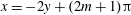 $x=-2y+(2m+1)\unicode[STIX]{x03C0}$
. Hence, the function
$x=-2y+(2m+1)\unicode[STIX]{x03C0}$
. Hence, the function
 $f(x)$
has precisely one local minimum and one local maximum on any contiguous half-open interval of length
$f(x)$
has precisely one local minimum and one local maximum on any contiguous half-open interval of length
 $2\unicode[STIX]{x03C0}$
.
$2\unicode[STIX]{x03C0}$
.

