


1. Introduction
Certain high-energy astrophysical sources are characterised by luminous and rapid flares of energetic radiation. In particular, these include blazars (e.g. Aharonian et al. Reference Aharonian, Akhperjanian, Bazer-Bachi, Behera, Beilicke, Benbow, Berge, Bernlöhr, Boisson and Bolz2007; Albert et al. Reference Albert, Aliu, Anderhub, Antoranz, Armada, Baixeras, Barrio, Bartko, Bastieri and Becker2007; Aleksić et al. Reference Aleksić, Antonelli, Antoranz, Backes, Barrio, Bastieri, Becerra González, Bednarek, Berdyugin and Berger2011; Abdo et al. Reference Abdo, Ackermann, Ajello, Allafort, Baldini, Ballet, Barbiellini, Bastieri, Bellazzini and Berenji2011b; Nalewajko Reference Nalewajko2013; Ackermann et al. Reference Ackermann, Anantua, Asano, Baldini, Barbiellini, Bastieri, Becerra Gonzalez, Bellazzini and Bissaldi2016) and the Crab pulsar wind nebula (Tavani et al. Reference Tavani, Bulgarelli, Vittorini, Pellizzoni, Striani, Caraveo, Weisskopf, Tennant, Pucella and Trois2011; Abdo et al. Reference Abdo, Ackermann, Ajello, Allafort, Baldini, Ballet, Barbiellini, Bastieri, Bechtol and Bellazzini2011a; Buehler et al. Reference Buehler, Scargle, Blandford, Baldini, Baring, Belfiore, Charles, Chiang, D'Ammando and Dermer2012; Lyubarsky Reference Lyubarsky2012; Mayer et al. Reference Mayer, Buehler, Hays, Cheung, Dutka, Grove, Kerr and Ojha2013; Striani et al. Reference Striani, Tavani, Vittorini, Donnarumma, Giuliani, Pucella, Argan, Bulgarelli, Colafrancesco and Cardillo2013). In these extreme astrophysical environments, magnetic fields may dominate even the local rest-mass energy density. Magnetic reconnection is considered a leading explanation for the efficient particle acceleration behind the dramatic gamma-ray flares of blazars (Giannios, Uzdensky & Begelman Reference Giannios, Uzdensky and Begelman2009; Nalewajko et al. Reference Nalewajko, Giannios, Begelman, Uzdensky and Sikora2011, Reference Nalewajko, Begelman, Cerutti, Uzdensky and Sikora2012; Giannios Reference Giannios2013; Sironi, Petropoulou & Giannios Reference Sironi, Petropoulou and Giannios2015; Petropoulou, Giannios & Sironi Reference Petropoulou, Giannios and Sironi2016). Through changes of the magnetic line topology, particles are accelerated in current sheets, converting magnetic energy into kinetic and thermal energy. In the case of the Crab pulsar wind nebula, the gamma-ray radiation spectral peaks can surpass the classical synchrotron radiation reaction limit ( ${\sim }160\ \textrm {MeV}$), which suggests a very efficient localised dissipation of magnetic energy that allows for rapid particle acceleration (Arons Reference Arons2012; Clausen-Brown & Lyutikov Reference Clausen-Brown and Lyutikov2012; Uzdensky, Cerutti & Begelman Reference Uzdensky, Cerutti and Begelman2011; Komissarov & Lyutikov Reference Komissarov and Lyutikov2011; Komissarov Reference Komissarov2012; Buehler & Blandford Reference Buehler and Blandford2014; Zrake Reference Zrake2016; Zrake & Arons Reference Zrake and Arons2017; Lyutikov et al. Reference Lyutikov, Komissarov, Sironi and Porth2018).
Numerical simulations based on the kinetic particle-in-cell (PIC) algorithm have demonstrated that relativistic reconnection in collisionless plasma is an efficient mechanism of magnetic energy dissipation and particle acceleration (Zenitani & Hoshino Reference Zenitani and Hoshino2001; Jaroschek et al. Reference Jaroschek, Treumann, Lesch and Scholer2004; Zenitani & Hoshino Reference Zenitani and Hoshino2007; Lyubarsky & Liverts Reference Lyubarsky and Liverts2008; Liu et al. Reference Liu, Li, Yin, Albright, Bowers and Liang2011; Bessho & Bhattacharjee Reference Bessho and Bhattacharjee2012; Kagan, Milosavljević & Spitkovsky Reference Kagan, Milosavljević and Spitkovsky2013; Guo et al. Reference Guo, Li, Daughton and Liu2014; Sironi & Spitkovsky Reference Sironi and Spitkovsky2014; Melzani et al. Reference Melzani, Walder, Folini, Winisdoerffer and Favre2014; Guo et al. Reference Guo, Liu, Daughton and Li2015, Reference Guo, Li, Li, Daughton, Zhang, Lloyd-Ronning, Liu, Zhang and Deng2016; Werner et al. Reference Werner, Uzdensky, Cerutti, Nalewajko and Begelman2016; Werner & Uzdensky Reference Werner and Uzdensky2017; Werner et al. Reference Werner, Uzdensky, Begelman, Cerutti and Nalewajko2018; Petropoulou & Sironi Reference Petropoulou and Sironi2018; Petropoulou et al. Reference Petropoulou, Sironi, Spitkovsky and Giannios2019; Guo et al. Reference Guo, Li, Daughton, Kilian, Li, Liu, Yan and Ma2019, Reference Guo, Li, Daughton, Li, Kilian, Liu, Zhang and Zhang2020), and that it can produce extreme radiative signatures – energetic, highly anisotropic and rapidly variable (Cerutti et al. Reference Cerutti, Werner, Uzdensky and Begelman2012, Reference Cerutti, Werner, Uzdensky and Begelman2013, Reference Cerutti, Werner, Uzdensky and Begelman2014; Kagan, Nakar & Piran Reference Kagan, Nakar and Piran2016; Nalewajko Reference Nalewajko2018a; Christie et al. Reference Christie, Petropoulou, Sironi and Giannios2018; Comisso, Sobacchi & Sironi Reference Comisso, Sobacchi and Sironi2020; Mehlhaff et al. Reference Mehlhaff, Werner, Uzdensky and Begelman2020; Ortuño-Macías & Nalewajko Reference Ortuño-Macías and Nalewajko2020). Most of these simulations were initiated from relativistic Harris-type current layers (Kirk & Skjaraasen Reference Kirk and Skjaraasen2003).
An alternative class of magnetostatic equilibria known as the ‘Arnold–Beltrami– Childress’ (ABC) magnetic fields (Arnold Reference Arnold1965) has been recently applied as an initial configuration for investigating relativistic magnetic dissipation (East et al. Reference East, Zrake, Yuan and Blandford2015). This configuration involves no kinetically thin current sheets, but is unstable to the so-called coalescence modes that lead to localised interactions of magnetic domains of opposite polarities, emergence of dynamical current layers, instantaneous particle acceleration and production of rapid flares of high-energy radiation. The overall process has been dubbed magnetoluminescence – a generic term for efficient and fast conversion of magnetic energy into radiation (Blandford et al. Reference Blandford, Yuan, Hoshino and Sironi2017).
Numerical simulations of ABC fields have been performed with relativistic magnetohydrodynamics and relativistic force-free (FF) algorithms (East et al. Reference East, Zrake, Yuan and Blandford2015). Detailed comparison between two-dimensional (2-D) and three-dimensional (3-D) ABC fields in the FF framework has been performed by Zrake & East (Reference Zrake and East2016). Some PIC simulations of 2-D ABC fields have been reported by Nalewajko et al. (Reference Nalewajko, Zrake, Yuan, East and Blandford2016) with the focus on the structure of current layers and particle acceleration, by Yuan et al. (Reference Yuan, Nalewajko, Zrake, East and Blandford2016) including synchrotron radiation reaction and radiative signatures and by Nalewajko, Yuan & Chruślińska (Reference Nalewajko, Yuan and Chruślińska2018) including synchrotron and inverse Compton radiation. The ABC fields have been also investigated in great detail (including PIC simulations) by Lyutikov et al. (Reference Lyutikov, Sironi, Komissarov and Porth2017a,Reference Lyutikov, Sironi, Komissarov and Porthb, Reference Lyutikov, Komissarov, Sironi and Porth2018) with application to the Crab Nebula flares. The first 3-D PIC simulations of ABC fields have been reported in Nalewajko (Reference Nalewajko2018b).
Previous works have established the following picture. The ABC fields simulated in periodic numerical grids are unstable to coalescence instability only if there exists a state of equal total magnetic helicity and lower total magnetic energy (East et al. Reference East, Zrake, Yuan and Blandford2015). The growth time scale of the linear coalescence instability is a fraction of the light crossing time scale that depends on the mean magnetisation (or equivalently on the typical Alfvén velocity) (Nalewajko et al. Reference Nalewajko, Zrake, Yuan, East and Blandford2016). The magnetic dissipation efficiency is determined primarily by the global magnetic field topology, and it is restricted in 2-D systems due to the existence of additional topological invariants (Zrake & East Reference Zrake and East2016). The dissipated magnetic energy is transferred to the particles, resulting in non-thermal high-energy tails of their energy distributions. These tails can be in most cases described as power laws with a power-law index, but more generally they can be characterised by the non-thermal number and energy fractions (Nalewajko et al. Reference Nalewajko, Zrake, Yuan, East and Blandford2016). With increasing initial magnetisation, the non-thermal tails become harder, containing higher number and energy fractions, similar to the results for Harris-layer reconnection (Guo et al. Reference Guo, Li, Daughton and Liu2014; Sironi & Spitkovsky Reference Sironi and Spitkovsky2014; Werner et al. Reference Werner, Uzdensky, Cerutti, Nalewajko and Begelman2016). A limitation of the ABC fields in comparison with the Harris layers is that the initial magnetisation is limited for a given simulation size by the minimum particle densities required to sustain volumetric currents.
The particle acceleration mechanisms of ABC fields, described in more detail in Nalewajko et al. (Reference Nalewajko, Zrake, Yuan, East and Blandford2016), Yuan et al. (Reference Yuan, Nalewajko, Zrake, East and Blandford2016) and Lyutikov et al. (Reference Lyutikov, Sironi, Komissarov and Porth2017a), show similarities to other numerical approaches to the problem of relativistic magnetic dissipation. During the linear stage of coalescence instability, kinetically thin current layers form and evolve very dynamically. The few particles that happen to straggle into one of those layers are accelerated by direct non-ideal reconnection electric fields ( $\boldsymbol {E}\boldsymbol {\cdot }\boldsymbol {B} \ne 0$,
  $|\boldsymbol {E}| > |\boldsymbol {B}|$). This is essentially the Zenitani & Hoshino (Reference Zenitani and Hoshino2001) picture of magnetic
  $X$-point, which is important also in large-scale simulations of Harris-layer reconnection in the sense that particles that pass through a magnetic
  $X$-point are most likely to eventually reach top energies (Sironi & Spitkovsky Reference Sironi and Spitkovsky2014; Guo et al. Reference Guo, Li, Daughton, Kilian, Li, Liu, Yan and Ma2019). The nonlinear stage of coalescence instability features slowly damped electric oscillations that gradually convert to particle energies. This can affect essentially all particles, as electric oscillations cross the entire simulation volume multiple times. Particles accelerated during the linear stage now propagate on wide orbits and can interact with electric perturbations at random angles. This is reminiscent of a Fermi process, in particular of the kind envisioned by Hoshino (Reference Hoshino2012). With a larger number of magnetic domains, the coalescence proceeds in multiple stages, with the successive current layers increasingly less regular. The system becomes chaotic more quickly and begins to resemble a decaying turbulence of the kind studied by Comisso & Sironi (Reference Comisso and Sironi2019).
As the previous PIC simulations of ABC fields were largely limited to the lowest unstable mode, in this work we present the results of new series of 2-D PIC simulations of ABC fields for different coherence lengths  $\lambda _0$ in order to understand how they affect the efficiency of magnetic dissipation and particle acceleration. Although the coalescence instability is rather fast, it is followed by slowly damped nonlinear oscillations, and hence our simulations are run for at least
  $25 L/c$ light crossing times for the system size
  $L$ to allow these oscillations to settle. Our simulations were performed at three different sizes. In addition we investigated the effects of numerical resolution and local particle anisotropy, in order to break the relation between the effective wavenumber and the mean initial magnetisation. We also compare our results with new 3-D simulations following the set-up described in Nalewajko (Reference Nalewajko2018b).
In § 2 we define the initial configuration of our simulations. Our results are presented in § 3, including spatial distributions of magnetic fields (§ 3.1), evolution of the total energy components (§ 3.2), conservation accuracy of the magnetic helicity (§ 3.3) and particle energy distributions (§ 3.4). A discussion is provided in § 4.
2. Simulation set-up
We perform a series of PIC simulations using the Zeltron codeFootnote 1 (Cerutti et al. Reference Cerutti, Werner, Uzdensky and Begelman2013) of 2-D periodic magnetic equilibria known as ABC fields (East et al. Reference East, Zrake, Yuan and Blandford2015). As opposed to the Harris layers, these initial configurations do not contain kinetically thin current layers. In two dimensions, there are two ways to implement ABC fields on a periodic grid, which we call diagonal and parallel, referring to the orientation of the separatrices between individual magnetic domains. The diagonal ABC field is defined as
 \begin{gather} B_x(x,y) = B_0\sin(2{\rm \pi} y/\lambda_0), \end{gather}
 \begin{gather}B_y(x,y) = B_0\cos(2{\rm \pi} x/\lambda_0), \end{gather}
 \begin{gather}B_z(x,y) = B_0[\sin(2{\rm \pi} x/\lambda_0)+\cos(2{\rm \pi} y/\lambda_0)], \end{gather}
where  $\lambda _0$ is the coherence length. The parallel ABC field can be obtained from the diagonal one through rotation by
  $45^{\circ }$ and increasing the effective wavenumber by a factor of
  $\sqrt {2}$:
 \begin{gather} B_x(x,y) = B_0[\sin(\sqrt{2}{\rm \pi}(x+y)/\lambda_0)+\sin(\sqrt{2}{\rm \pi}(x-y)/\lambda_0)]/\sqrt{2}, \end{gather}
 \begin{gather}B_y(x,y) = B_0[\sin(\sqrt{2}{\rm \pi}(x-y)/\lambda_0)-\sin(\sqrt{2}{\rm \pi}(x+y)/\lambda_0)]/\sqrt{2}, \end{gather}
 \begin{gather}B_z(x,y) = B_0[\cos(\sqrt{2}{\rm \pi}(x+y)/\lambda_0)-\cos(\sqrt{2}{\rm \pi}(x-y)/\lambda_0)]. \end{gather}
With this, both the diagonal and parallel configurations satisfy the Beltrami condition  $\boldsymbol {\nabla }\times \boldsymbol {B} = -(2{\rm \pi} /\lambda _0)\boldsymbol {B}$. In all cases, the mean squared magnetic field strength is
  $\langle B^2\rangle = 2B_0^2$ and the maximum magnetic field strength is
  $B_{\max } = 2B_0$.
These magnetic fields are maintained in an initial equilibrium by volumetric current densities  $\boldsymbol {j}(\boldsymbol {x}) = -(c/2\lambda _0)\boldsymbol {B}(\boldsymbol {x})$ provided by locally anisotropic particle distribution (for details, see Nalewajko et al. (Reference Nalewajko, Zrake, Yuan, East and Blandford2016) and Nalewajko (Reference Nalewajko2018b)). The ABC fields are characterised by vanishing divergence of the electromagnetic stress tensor
  $\partial _iT_\textrm {EM}^{ij} = 0$ (equivalent to the vanishing
  $\boldsymbol {j}\times \boldsymbol {B}$ force), which implies uniform gas pressure that can be realised with uniform temperature
  $T$ and uniform gas density
  $n$. We chose the initial particle energy distribution to be a Maxwell–Jüttner distribution of relativistic temperature
  $\varTheta = kT/mc^2 = 1$, and hence the mean particle energy is
  $\langle \gamma \rangle \simeq 3.37$ and the mean particle velocity is
  $\langle \beta \rangle \simeq 0.906$. The gas density (including both electrons and positrons) is given by
 \begin{equation} n = \frac{3B_0}{2e \tilde{a}_1\langle\beta\rangle \lambda_0}, \end{equation}
where  $\tilde {a}_1 \leqslant 1/2$ is a constant that normalises the dipole moment of the local particle distribution. We chose
  $\tilde {a}_1 = 1/4$ as a standard value, but we investigate the effect of reduced local particle anisotropy with lower values of
  $\tilde {a}_1$ that result in higher particle densities and lower magnetisation values. The initial kinetic energy density is
 \begin{equation} u_{\textrm{kin},\textrm{ini}} = \langle\gamma\rangle nm_{e}c^2 \simeq \frac{6{\rm \pi}\langle\gamma\rangle}{\tilde{a}_1\varTheta\langle\beta\rangle} \left(\frac{\rho_0}{\lambda_0}\right) \langle u_{B,\textrm{ini}}\rangle, \end{equation}
where  $\rho _0 = \varTheta m_\textrm {e} c^2/(eB_0)$ is the nominal gyroradius and
  $\langle u_{B,\textrm {ini}}\rangle = B_0^2/4{\rm \pi}$ is the initial mean magnetic energy density. The initial mean hot magnetisation is given by
 \begin{equation} \langle\sigma_\textrm{ini}\rangle = \frac{\langle B^2\rangle}{4{\rm \pi} w} = \frac{\tilde{a}_1\varTheta\langle\beta\rangle}{3{\rm \pi} (\langle\gamma\rangle+\varTheta)} \left(\frac{\lambda_0}{\rho_0}\right), \end{equation}
where  $w = (\langle \gamma \rangle +\varTheta )nm_{e}c^2$ is the relativistic enthalpy density. For
  $\varTheta = 1$, we have
  $\langle \sigma _\textrm {ini}\rangle \simeq (4\tilde {a}_1)(\lambda _0/182\rho _0)$.
We performed simulations of either diagonal or parallel ABC fields and for different wavenumbers  $k$ (
$k$ ( $k = L/\lambda _0$ for diagonal configuration and
  $k = L/\sqrt {2}\lambda _0$ for parallel configuration). For instance, a simulation labelled diag_k2 is initiated with a diagonal ABC field with
  $L/\lambda _0 = 2$. In order to verify the scaling of our results, we performed series of simulations for three sizes of numerical grids: small (s) for
  $N_x = N_y = 1728$; medium (m) for
  $N_x = N_y = 3456$; and large (l)
  $N_x = N_y = 6912$. For numerical resolution
  $\Delta x = \Delta y = L/N_x$, where
  $L$ is the physical system size, we chose a standard value of
  $\Delta x = \rho _0/2.4$, but we investigated the effect of increased resolution on the medium numerical grid. The numerical time step was chosen as
  $\Delta t = 0.99(\Delta x/\sqrt {2}c)$. All of our simulations were performed for at least
  $25 L/c$ light crossing times. In each case we used 128 macroparticles (including both species) per cell.
We also performed two new 3-D simulations for the cases diag_k2 and diag_k4, following the configuration described in Nalewajko (Reference Nalewajko2018b), but extending them to  $25 L/c$. In this case we chose the following parameter values:
  $N_x = N_y = N_z = 1152$,
  $\Delta x = \Delta y = \Delta z = \rho _0/1.28$,
  $\tilde {a}_1 = 0.2$ and 16 macroparticles per cell.
3. Results
The key parameters of our large simulations are listed in table 1, where we report basic results describing global energy transformations that are discussed in § 3.2, and particle energy distributions that are discussed in § 3.4.
Table 1. Global parameters of energy conversion and particle acceleration compared for the 2-D and 3-D simulations. The initial values denoted with subscript ‘ini’ are measured at  $t=0$ and the final values (‘fin’) are averaged over
  $20 \leqslant ct/L \leqslant 25$. The initial mean hot magnetisation
  $\langle \sigma _\textrm {ini}\rangle$ is computed from (2.9). The initial magnetic energies
  $\mathcal {E}_{B,\textrm {ini}}$ are normalised to the total system energy
  $\mathcal {E}_\textrm {tot}$. The magnetic dissipation efficiency is defined as
  $\epsilon _\textrm {diss} = 1-\mathcal {E}_{B,\textrm {fin}}/\mathcal {E}_{B,\textrm {ini}}$. We report the peak value
  $\tau _{E,\textrm {peak}}$ of the linear growth time scale
  $\tau _E$ of electric energy, which scales like
  $\mathcal {E}_{E} \propto \exp (ct/L\tau _E)$. For the final particle energy distributions, we report: the power-law index
  $p$, the maximum Lorentz factor
  $\gamma _{\max }$ and the non-thermal particle energy fraction
  $f_E$.

3.1. Spatial distribution of magnetic fields
Figure 1 compares the initial ( $ct/L = 0$), intermediate (
 $ct/L \simeq 4$) and final (
 $ct/L \simeq 25$) configurations of the out-of-plane magnetic field component
  $B_z$. The initial configurations have the form of periodic grids of
  $B_z$ minima (blue) and maxima (red). The case diag_k1 is the only one that represents a stable equilibrium, as it involves only one minimum and one maximum of
  $B_z$. The case para_k1 (investigated in detail in Nalewajko et al. (Reference Nalewajko, Zrake, Yuan, East and Blandford2016) and Yuan et al. (Reference Yuan, Nalewajko, Zrake, East and Blandford2016)) begins with two minima and two maxima of
  $B_z$, by
  $ct/L \simeq 4$ it is just entering the linear instability stage and the final state appears very similar to the case diag_k1, although the domains of positive and negative
  $B_z$ are still slightly perturbed. As we increase
  $L/\lambda _0$, throughout the case of para_k4, the intermediate states become more evolved, at further stages of magnetic domain coalescence, while the final states in all cases consist of single positive and negative
  $B_z$ domains. We notice that these domains become separated by increasingly broad bands of
  $B_z \simeq 0$.

Figure 1. Spatial distributions of the out-of-plane magnetic field component  $B_z$ for ABC fields of different initial topologies. Each column of panels compares the initial configuration at
  $ct/L = 0$ (a) with an intermediate state at
  $ct/L \simeq 4$ (b) and with the final state at
  $ct/L \simeq 25$ (c).
3.2. Total energy transformations
The initial configurations investigated here involve various levels of magnetic energy  $\mathcal {E}_{B,\textrm {ini}}$ as fractions of the total energy
  $\mathcal {E}_{\textrm {tot}}$. The initial magnetic energy fraction decreases with increasing
  $L/\lambda _0$ and increases with the system size. Our simulations probe the range of
  $\mathcal {E}_{B,\textrm {ini}}/\mathcal {E}_\textrm {tot}$ values from 0.19 to 0.88. Related to the initial magnetic energy fraction is the initial mean hot magnetisation
  $\langle \sigma _\textrm {ini}\rangle$ (see (2.9)), which in our simulations takes values from 0.35 to 11.2.
Time evolutions of the magnetic energy fractions are presented in figure 2(a). In all studied cases, the magnetic energy experiences a sudden decrease followed by a slow settling. As the settling is largely complete by  $t = 20L/c$, we measure the final magnetic energy fraction
  $\mathcal {E}_{B,\textrm {fin}}$ as the average over the
  $20 < ct/L < 25$ period. We define the final magnetic dissipation efficiency as
  $\epsilon _{\textrm {diss},\textrm {fin}} = 1 - \mathcal {E}_{B,\textrm {fin}}/\mathcal {E}_{B,\textrm {ini}}$. Figure 2(b) shows that
  $\epsilon _{\textrm {diss},\textrm {fin}}$ is a function of magnetic topology parameter
  $L/\lambda _0$, almost independent of the system size
  $L$ (although it is slightly lower for reduced values of
  $\tilde {a}_1$). For large values of
  $L/\lambda _0$, magnetic dissipation efficiency appears to saturate at the level of
  $\epsilon _\textrm {diss} \sim 0.6$. We have fitted the large and medium 2-D results for the standard values of
  $\tilde {a}_1$ and
  $\rho _0/\Delta x$ with a relation
  $\epsilon _\textrm {diss} = \epsilon _0 - \epsilon _2(\lambda _0/L)^2$, finding
  $\epsilon _0 \simeq 0.62$ and
  $\epsilon _2 \simeq 0.70$.

Figure 2. (a) Time evolution of the magnetic energy  $\mathcal {E}_{B}$ as a fraction of the total energy
  $\mathcal {E}_\textrm {tot}$ for the medium (thin solid lines) and large (thick solid lines) simulation sizes. The thick dashed lines indicate two 3-D simulations. The line colour indicates the effective wavenumber
  $L/\lambda _0$, as shown in the right-hand panel. (b) Final magnetic dissipation efficiency
  $\epsilon _{\textrm {diss},\textrm {fin}} = 1 - \mathcal {E}_{B,\textrm {fin}} / \mathcal {E}_{B,\textrm {ini}}$ (evaluated at
  $20 < ct/L < 25$) as a function of the effective wavenumber of initial magnetic configuration
  $L/\lambda _0$. The large/medium/small circles indicate new results obtained from large/medium/small simulations, the plus symbols indicate simulations for non-standard values of
  $\tilde {a}_1$, the cross symbols indicate simulations for non-standard values of
  $\rho _0/\Delta x$ and the stars indicate 3-D simulations. The symbol colours indicate the effective wavenumber
  $L/\lambda _0$. The black dashed line shows a
  $1-\lambda _0/L$ relation predicted by the relaxation theorem of Taylor (Reference Taylor1974) and matching the 3-D results, and the magenta dashed line shows a
 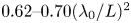 $0.62 \text {--} 0.70(\lambda _0/L)^2$ relation fitted to the 2-D results.
Also shown in figure 2 are analogous results for two 3-D simulations. These results are consistent with a relation 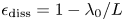 $\epsilon _\textrm {diss} = 1 - \lambda _0/L$ predicted by the relaxation theorem of Taylor (Reference Taylor1974).
The initial sudden decrease of the magnetic energy is mediated by rapid growth of the electric energy. Time evolutions of the electric energy  $\mathcal {E}_{E}$ as a fraction of the initial magnetic energy
  $\mathcal {E}_{B,\textrm {ini}}$ are presented in figure 3(a). In all studied cases we find an episode of rapid exponential growth of the electric energy, an indication of linear instability known as coalescence instability (East et al. Reference East, Zrake, Yuan and Blandford2015). We indicate moments of peak electric energy growth time scale
  $\tau _{E,\textrm {peak}}$ (defined by
  $\mathcal {E}_{E} \propto \exp (ct/L\tau _{E})$). Figure 3(b) compares the values of
  $\tau _{E,\textrm {peak}}$, multiplied by
  $L/\lambda _0$, as a function of the initial mean magnetisation
  $\langle \sigma _\textrm {ini}\rangle$. Combining our 2-D results with the previous simulations for the case para_k1 reported in Nalewajko et al. (Reference Nalewajko, Zrake, Yuan, East and Blandford2016), the relation between
  $\tau _{E,\textrm {peak}}$ and
  $\langle \sigma _\textrm {ini}\rangle$ for the standard values of
  $\tilde {a}_1$ and
  $\rho _0/\Delta x$ has been fitted as
 \begin{equation} \tau_{E,\textrm{peak}} \simeq \frac{0.233\pm 0.005}{(L/\lambda_0)\beta_{A,\textrm{ini}}^3}, \end{equation}
where 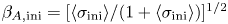 $\beta _{A,\textrm {ini}} = [\langle \sigma _\textrm {ini}\rangle /(1+\langle \sigma _\textrm {ini}\rangle )]^{1/2}$ is the characteristic value of initial Alfvén velocity. The four 3-D simulations (including two new full runs and two shorter runs from

Figure 3. (a) Time evolution of the electric energy  $\mathcal{E}_E$ as a fraction of the initial magnetic energy
  $\mathcal {E}_{B,\textrm {ini}}$. The line types are the same as in figure 2(a). Moments of minimum growth time scale are indicated with filled symbols. (b) Minimum growth time scales for the total electric energy
  $\tau _{E}$ as a function of the initial mean magnetisation
  $\langle \sigma _\textrm {ini}\rangle$. The symbol types are the same as in figure 2(b); in addition the blue diamonds indicate the para_k1 simulations from Nalewajko et al. (Reference Nalewajko, Zrake, Yuan, East and Blandford2016), and original shorter 3-D runs from Nalewajko (Reference Nalewajko2018b) are indicated. The black dashed line shows a
  $\beta _{A}^{-3}$ trend (see (3.1)) fitted to all 2-D results. The blue dashed line shows a different trend (see (4.1)) suggested previously by Nalewajko et al. (Reference Nalewajko, Zrake, Yuan, East and Blandford2016).
Nalewajko (Reference Nalewajko2018b)) show longer growth time scales compared with their 2-D counterparts, with the cases para_k4 being strongly affected by the noise component of the electric field.
3.3. Conservation of total energy and magnetic helicity
Figure 4 shows the conservation accuracy for the total system energy  $\mathcal {E}_\textrm {tot}$ and total magnetic helicity
  $\mathcal {H} = \int H\,\textrm {d}V$ (where
  $H = \boldsymbol {A}\boldsymbol {\cdot }\boldsymbol {B}$ with
  $\boldsymbol {A}$ the magnetic vector potential). The conservation accuracy for parameter
  $X$ is defined as
  $\delta _X \equiv \max |X(ct<25L)/X(t=0)-1|$. The conservation accuracy of total energy
  $\delta _\mathcal {E}$ is presented as a function of modified magnetisation parameter
  $\sigma _{\mathcal {E}} \equiv \langle \sigma _\textrm {ini}\rangle (2.4\Delta x/\rho _0)^{-3/4} (L/2880\rho _0)^{-3/4}$. For
  $1 < \sigma _{\mathcal {E}} < 6$ (essentially for
  $L/\lambda _0 \gtrsim 2\sqrt {2}$), energy conservation accuracy scales like
  $\delta _\mathcal {E} \propto \sigma _\mathcal {E}^{-5/2} \propto \langle \sigma _\textrm {ini}\rangle ^{-5/2} (\Delta x/\rho _0)^{15/8 \simeq 2} (L/\rho _0)^{15/8 \simeq 2}$, reaching the value of
  $\simeq 0.02$ for
  $\sigma _\mathcal {E} \simeq 1$. For
  $\sigma _\mathcal {E} > 6$, energy conservation accuracy is found to be of the order of
  $\delta _\mathcal {E} \sim 3\times 10^{-4}$. In the 3-D cases, energy conservation is found to be worse by factor
  $\simeq 30$ as compared with the 2-D results for the same value of
  $\sigma _\mathcal {E}$.

Figure 4. Conservation accuracies of total energy  $\delta _\mathcal {E}$ (a) and total magnetic helicity
  $\delta _\mathcal {H}$ (b) as functions of modified magnetisation parameters
  $\sigma _\mathcal {E}$ and
  $\sigma _\mathcal {H}$, respectively, chosen to minimise scatter around the suggested trends (dashed lines;
  $\sigma _\mathcal {E}^{-5/2}$ and
  $\sigma _\mathcal {H}^{-2}$, respectively). See the main text for details. The symbol types are the same as in figure 2(b).
The conservation accuracy of total magnetic helicity  $\delta _\mathcal {H}$ is presented as a function of a different modified magnetisation parameter
  $\sigma _\mathcal {H} \equiv \langle \sigma _\textrm {ini}\rangle / (4\tilde {a}_1) \simeq \lambda _0/182\rho _0$ (the latter assuming
  $\varTheta =1$). For
  $\sigma _\mathcal {H} < 2.5$, magnetic helicity conservation accuracy scales like
  $\delta _\mathcal {H} \propto \sigma _\mathcal {H}^{-2} \propto (\lambda _0/\rho _0)^{-2}$, reaching the value of
  $\simeq 0.1$ for
  $\sigma _\mathcal {H} \simeq 0.4$. For
  $\sigma _\mathcal {H} > 2.5$ (essentially for
  $L/\lambda _0 \lesssim 2$), we find that simulations with reduced values of
  $\tilde {a}_1$ appear to follow the same trend; however, large and medium simulations with standard
  $\tilde {a}_1$ value show worse conservation of the order of
  $\delta _\mathcal {H} \sim 3\times 10^{-3}$. In the 3-D cases, magnetic helicity conservation is found to be worse by factor
  $\sim 12$ as compared with the 2-D results for the same value of
  $\sigma _\mathcal {H}$.
3.4. Particle energy distributions
Figure 5 shows the particle momentum distributions  $N(u)$ (closely related to the energy distributions for
  $u = \sqrt {\gamma ^2-1} \gg 1$) for the final states of the medium and large 2-D simulations, as well as the 3-D simulations (averaged over the time range of
  $20 < ct/L < 25$). The non-evolving case diag_k1 is equivalent to the initial Maxwell–Jüttner distribution. A high-energy excess is evident in all other cases.

Figure 5. Momentum distributions  $u^2 N(u)$ of electrons and positrons averaged over the time period
  $20 < ct/L < 25$. The line types are the same as in figure 2(a).
There are several ways to characterise this excess component. In most cases, a power-law section can be clearly identified. Accurate evaluation of the corresponding power-law index  $p$ (such that
  $N(u) \propto u^{-p}$) is in general complicated, as it requires fitting analytical functions that properly represent the high-energy cutoff (Werner et al. Reference Werner, Uzdensky, Cerutti, Nalewajko and Begelman2016). Here, in order to avoid those complications, we estimate a power-law index using a compensation method, multiplying the measured distribution by
  $u^p$ with different
  $p$ values to obtain the broadest and most balanced plateau section. The accuracy of this method is estimated at
  ${\pm } 0.05$. The best values of
  $p$ estimated for our simulations are reported in table 1. No power-law sections could be identified for certain cases with low initial magnetisations
  $\langle \sigma _\textrm {ini}\rangle < 1$. The hardest spectrum with
  $p \simeq 2.4$ has been found for the large simulation para_k1. A similar spectrum with
  $p \simeq 2.45$ (re-examined with the same method) has been obtained in previous simulations for the case para_k1 reported in Nalewajko et al. (Reference Nalewajko, Zrake, Yuan, East and Blandford2016) and characterised by slightly higher initial magnetisation of
  $\langle \sigma _\textrm {ini}\rangle = 12.4$.
Figure 6(a) shows the power-law index  $p$ as a function of the initial magnetic energy fraction
  $\mathcal {E}_{B,\textrm {ini}}/\mathcal {E}_\textrm {tot}$. The value of
  $p$ is strongly anti-correlated with
  $\mathcal {E}_{B,\textrm {ini}}/\mathcal {E}_\textrm {tot}$, independent of the simulation size, with a Pearson correlation coefficient of
  $\simeq -0.98$. A linear trend has been fitted to the results of 2-D simulations with standard values of
  $\tilde {a}_1$ and
  $\rho _0/\Delta x$, including the previous para_k1 simulations from Nalewajko et al. (Reference Nalewajko, Zrake, Yuan, East and Blandford2016):
 \begin{equation} p \simeq ({-}3.9 \pm 0.2) \frac{\mathcal{E}_{B,\textrm{ini}}}{\mathcal{E}_\textrm{tot}} + (5.8 \pm 0.1). \end{equation}
Also shown are results for two 3-D simulations showing particle distributions slightly steeper as compared with 2-D simulations with comparable initial magnetic energy fractions.

Figure 6. (a) Power-law index  $p$ of the momentum distribution
  $N(u) \propto u^{-p}$ as a function of the initial magnetic energy fraction
  $\mathcal {E}_{B,\textrm {ini}}/\mathcal {E}_\textrm {tot}$. The black dashed line shows a linear trend fitted to all 2-D results. (b) Non-thermal energy fraction
  $f_E$ as a function of a modified magnetisation parameter
  $\sigma _f$. The dashed lines indicate two trends:
  $\propto \sigma _f^{3/4}$ (blue) and
  $\propto \sigma _f^{2}$ (brown). For both panels, the symbol types are the same as in figure 3(b).
The high-momentum excess component of the particle distribution can be alternatively characterised by the maximum particle energy reached  $\gamma _{\max }$. Here, the value of
  $\gamma _{\max }$ is evaluated at the fixed level of
  $10^{-3}$ of the
  $u^2 N(u)$ distribution normalised to peak at unity (cf. the bottom edge of figure 5). The final values of
  $\gamma _{\max }$ for our large simulations are reported in table 1. The highest value of
  $\gamma _{\max } \simeq 1620$ has been found for the large simulation para_k2. For the cases where the power-law index
  $p$ could be evaluated (note that
  $\gamma _{\max }$ can always be evaluated),
  $\log \gamma _{\max }$ is strongly anti-correlated with
  $p$, with a Pearson correlation coefficient of
  $\simeq -0.99$.
Yet another approach to the high-momentum excess is to fit and subtract a low-momentum Maxwell–Jüttner component and to calculate the non-thermal fractions of particle number  $f_n$ and particle energy
  $f_E$ contained in the remaining excess. This fitting was performed using the weighted least squares method with the weights proportional to
  $u^{-2}$. In all cases, the non-thermal number fractions were found to be closely related to the energy fractions as
  $f_n \simeq f_E/3.5$. The values of non-thermal energy fractions
  $f_E$ for our simulations are reported in table 1. The highest value of
  $f_E \simeq 56\,\%$ has been found for the large simulation diag_k1. For the cases where
  $p$ could be evaluated,
  $f_E$ is anti-correlated with
  $p$, with a Pearson correlation coefficient of
  $\simeq -0.93$.
Figure 6(b) shows the non-thermal energy fraction  $f_E$ versus another modified magnetisation parameter
  $\sigma _f \equiv \langle \sigma _\textrm {ini}\rangle (4\tilde {a}_1)^{1/2}$. We also indicate the
  $f_E \propto \langle \sigma _\textrm {ini}\rangle ^{3/4}$ trend suggested by Nalewajko et al. (Reference Nalewajko, Zrake, Yuan, East and Blandford2016) and re-fitted only to the para_k1 results (deep blue symbols). We confirm that this trend describes the para_k1 results reasonably well; however, it is not followed by the high-
 $(L/\lambda _0)$ cases that probe lower magnetisation values
  $\sigma _f < 1$. In the particular case of
  $L/\lambda _0 = 8\sqrt {2}$ (brown symbols), the values of
  $f_E$ decrease faster with decreasing
  $\sigma _f$, roughly like
  $f_E \propto \sigma _f^{2}$ for
  $\sigma _f < 1$. For intermediate magnetisation values
  $1 < \sigma _f < 10$, the values of
  $f_E$ for
  $L/\lambda _0 > \sqrt {2}$ are systematically higher as compared with the para_k1 trend line. The 3-D simulations produced
  $f_E$ values that are consistent with (in the case diag_k2) or somewhat lower than (in the case diag_k4) the 2-D results.
We use the final non-thermal energy fractions  $f_E$ to divide the global energy gain of the particles into the non-thermal and thermal parts:
 \begin{gather} \Delta\mathcal{E}_\textrm{nth} =f_E\,\mathcal{E}_{\textrm{kin},\textrm{fin}}, \end{gather}
 \begin{gather}\Delta\mathcal{E}_\textrm{th} = (1-f_E)\mathcal{E}_{\textrm{kin},\textrm{fin}} - \mathcal{E}_{\textrm{kin},\textrm{ini}}, \end{gather}
where  $\mathcal {E}_{\textrm {kin},\textrm {ini}} = \mathcal {E}_\textrm {tot} - \mathcal {E}_{B,\textrm {ini}}$ and
  $\mathcal {E}_{\textrm {kin},\textrm {fin}} \simeq \mathcal {E}_\textrm {tot} - \mathcal {E}_{B,\textrm {fin}}$, since by
  $ct = 25L$ the total electric energy that mediates the dissipation of magnetic energy decreases to the level of
 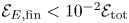 $\mathcal {E}_{E,\textrm {fin}} < 10^{-2}\mathcal {E}_\textrm {tot}$. The two components of particle energy gain are presented in figure 7 as functions of yet two other modified magnetisation parameters
  $\sigma _\textrm {th} \equiv \langle \sigma _\textrm {ini}\rangle (4\tilde {a}_1)^{-1/2} (L/\lambda _0)^{3/4} (2.4\Delta x/\rho _0)^{3/4}$ and
  $\sigma _\textrm {nth} \equiv \langle \sigma _\textrm {ini}\rangle (4\tilde {a}_1)^{1/2} (L/\lambda _0)^{-1/4} (2.4\Delta x/\rho _0)^{-1/4}$, respectively. We find that the cases of para_k1 (deep blue symbols) stand out from other cases, having significantly lower thermal energy gains, suggesting that they are limited by the magnetic topology. On the other hand, their non-thermal energy gains are comparable to other cases, but achieved at significantly higher values of
  $\sigma _\textrm {nth}$. Power-law trends can be suggested only for sufficiently high wavenumbers (
 $L/\lambda _0 \gtrsim 4\sqrt {2}$):
  $\Delta \mathcal {E}_\textrm {th} \propto \sigma _\textrm {th}^{1/3}$ and
 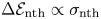 $\Delta \mathcal {E}_\textrm {nth} \propto \sigma _\textrm {nth}$, respectively. However, in the diag_k8 cases (brown symbols), a steeper trend for the non-thermal energy gain
 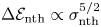 $\Delta \mathcal {E}_\textrm {nth} \propto \sigma _\textrm {nth}^{5/2}$ is apparent for low magnetisation values
  $\sigma _\textrm {nth} < 0.25$. The highest value of
 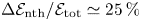 $\Delta \mathcal {E}_\textrm {nth} / \mathcal {E}_\textrm {tot} \simeq 25\,\%$ is obtained for our large simulation diag_k2.

Figure 7. Global gain of the particle energy divided into thermal  $\Delta \mathcal {E}_\textrm {th}$ (a) and non-thermal
  $\Delta \mathcal {E}_\textrm {nth}$ (b) components, normalised to the total energy
  $\mathcal {E}_\textrm {tot}$, as functions of modified magnetisation parameters
  $\sigma _\textrm {th}$ and
  $\sigma _\textrm {nth}$, respectively, chosen to minimise scatter around suggested trends (dashed black lines)
  $\propto \sigma _\textrm {th}^{1/3}$ and
  $\propto \sigma _\textrm {nth}$, respectively. The symbol types are the same as in figure 3(b).
4. Discussion
Our new results extend the previous study of 2-D PIC simulations of ABC fields for the para_k1 case in the non-radiative regime (Nalewajko et al. Reference Nalewajko, Zrake, Yuan, East and Blandford2016), and connect it with a study of 3-D PIC simulations for the cases diag_k2 and diag_k4 (Nalewajko Reference Nalewajko2018b). They can also be compared with the FF simulations of ABC fields presented in Zrake & East (Reference Zrake and East2016). In particular, the magnetic dissipation efficiency in the FF limit in two dimensions has been estimated at  $\epsilon _\textrm {diss} \simeq 70\,\%$, while our results suggest
  $\epsilon _\textrm {diss} \simeq 62\,\%$ in the limit of
  $L/\lambda _0 \gg 1$. It should be noted, however, that in PIC simulations this limit forces us towards lower magnetisation values.
In Nalewajko et al. (Reference Nalewajko, Zrake, Yuan, East and Blandford2016), a relation between the electric energy growth time scale  $\tau _{E,\textrm {peak}}$ and the initial characteristic hot magnetisation
  $\sigma _\textrm {hot}$ was suggested in the following form:
 \begin{equation} \tau_{E,\textrm{peak}} \simeq \frac{0.13}{v_{A}(0.21\sigma_\textrm{hot})}, \end{equation}
where  $v_{A}(\sigma ) \equiv [\sigma /(1+\sigma )]^{1/2}$ was treated as a function in the form of Alfvén velocity of arbitrarily scaled argument
  $\sigma$, and
  $\sigma _\textrm {hot} \equiv \langle \sigma _\textrm {ini}\rangle /2$ was a characteristic value of hot magnetisation based on
  $B_0^2$ instead of the mean value
  $\langle B^2\rangle$ used here.Footnote 2 The above relation is shown in figure 3(b) with a dashed blue line (cf. figure 3 of Nalewajko et al. Reference Nalewajko, Zrake, Yuan, East and Blandford2016). We can see that the previously suggested trend agrees very well with the previous measurements from Nalewajko et al. (Reference Nalewajko, Zrake, Yuan, East and Blandford2016), and is very close to the new trend line in the range
  $1.5 < \langle \sigma _\textrm {ini}\rangle < 12.5$. However, the previous trend predicts significantly shorter growth time scales for low magnetisation values
  $\langle \sigma _\textrm {ini}\rangle < 1$ that is probed here with simulations for
  $L/\lambda _0 \geqslant 4\sqrt {2}$.
Our new scaling described by (3.1) is more natural, without arbitrary scaling parameters. It suggests that in the FF limit, when  $\langle \sigma _\textrm {ini}\rangle \to \infty$ and
  $\beta _{A,\textrm {ini}} \to 1$, we should expect that the growth time scale should become
  $\tau _{E,\textrm {FF}} \simeq 0.233/(L/\lambda _0)$. For
  $L/\lambda _0 = \sqrt {2}$, this would yield
  $\tau _{E,\textrm {FF}} \simeq 0.16$, somewhat longer than
  $\tau _{E,\textrm {FF}} \simeq 0.13$ indicated by Nalewajko et al. (Reference Nalewajko, Zrake, Yuan, East and Blandford2016). As for why
  $\tau _{E,\textrm {peak}} (L/\lambda _0)$ should scale with
  $\beta _{A,\textrm {ini}}^{-3}$ requires a theoretical investigation of the linear coalescence instability beyond the FF limit, with proper treatment of magnetic nulls, which is beyond the scope of this work.
We can only partially confirm a relation between non-thermal energy fraction and initial mean hot magnetisation  $f_E \propto \langle \sigma _\textrm {ini}\rangle ^{3/4}$ originally suggested in Nalewajko et al. (Reference Nalewajko, Zrake, Yuan, East and Blandford2016). This relation appears to hold for the para_k1 case, including new simulations extending into the
  $\langle \sigma _\textrm {ini}\rangle \sim 1$ regime, and possibly also for higher values of
  $L/\lambda _0$ as long as
  $\sigma _f > 1$ (see figure 6b). However, for the cases where a power-law index
  $p$ can be determined, a simple linear relation holds between
  $p$ and the initial magnetic energy fraction
  $\mathcal {E}_{B,\textrm {ini}} / \mathcal {E}_\textrm {tot}$ (see (3.2)), at least over the studied range
  $0.3 < \mathcal {E}_{B,\textrm {ini}} / \mathcal {E}_\textrm {tot} < 0.9$ (see figure 6a).
We have introduced several modified magnetisation parameters, as combinations of the initial mean magnetisation  $\langle \sigma _\textrm {ini}\rangle$ with other input parameters, in order to describe the scalings of global output parameters. The particular formulae for the modified magnetisations were chosen in order to minimise scatter around the suggested trends, with the exponents of
  $\Delta x/\rho _0$,
  $L/\rho _0$,
  $L/\lambda _0$ and
  $\tilde {a}_1$ estimated empirically with an accuracy of
  $\sim \pm 1/4$. The energy conservation accuracy for ABC fields simulated with the Zeltron code is found to scale roughly like
  $\delta _\mathcal {E} \propto \langle \sigma _\textrm {ini}\rangle ^{-5/2} (\Delta x/\rho _0)^2 (L/\rho _0)^2$, not sensitive to
  $\lambda _0$. This is different from the reference case of uniform magnetic field, in which we found
  $\delta _\mathcal {E} \propto \langle \sigma _\textrm {ini}\rangle ^{-1} (\Delta x/\rho _0)^2$, independent of
  $L$. On the other hand, the magnetic helicity conservation accuracy is found to scale like
  $\delta _\mathcal {H} \propto (\lambda _0/\rho _0)^{-2}$, but it is not sensitive to
  $\Delta x/\rho _0$ or
  $L/\rho _0$. This is in contrast to the FF simulations of Zrake & East (Reference Zrake and East2016), in which
  $\delta _\mathcal {H} \propto (\Delta x)^{2.8}$. Further investigation is required in order to explain these differences.
For the non-thermal energy fraction  $f_{E}$, the scaling with initial mean magnetisation
  $\langle \sigma _\textrm {ini}\rangle$ is rather ambiguous. Only in the special case of
  $L/\lambda _0 = \sqrt {2}$ do we have sufficient range of
  $\langle \sigma _\textrm {ini}\rangle$ values to claim that
  $f_{E} \propto \langle \sigma _\textrm {ini}\rangle ^{3/4}$; this scaling is improved by additional dependence on the particle anisotropy level
  $\tilde {a}_1$. The scalings of thermal and non-thermal kinetic energy gains,
  $\Delta \mathcal {E}_\textrm {th}$ and
  $\Delta \mathcal {E}_\textrm {nth}$, respectively, can in principle be derived from the scalings of
  $f_{E}$ and magnetic dissipation efficiency
  $\epsilon _\textrm {diss}$. The ambiguity of the
  $f_{E}$ scaling makes it not straightforward to predict in detail the scalings of
  $\Delta \mathcal {E}_\textrm {th}$ and
  $\Delta \mathcal {E}_\textrm {nth}$.
The initial mean hot magnetisation  $\langle \sigma _\textrm {ini}\rangle$ of ABC fields with relativistically warm plasma (
 $\varTheta = 1$) is strongly limited by the simulation size, especially if one would like to resolve numerically all the fundamental length scales, in particular the nominal gyroradius
  $\rho _0$. For a given effective wavenumber
  $L/\lambda _0$, higher values of
  $\langle \sigma _\textrm {ini}\rangle$ can only be reached by increasing the system size
  $L/\rho _0$.Footnote 3 It can be expected that larger simulations would show more effective non-thermal particle acceleration with harder high-energy tails indicated by higher values of non-thermal energy fractions
  $f_e$ and lower values of power-law indices
  $p$. Eventually, at sufficiently high
  $\langle \sigma _\textrm {ini}\rangle$, and with
  $L/\lambda _0 \geqslant 2$, it should be possible to achieve particle distributions dominated energetically by the high-energy particles, with
  $p < 2$, as has been demonstrated in the case of Harris-layer reconnection (Guo et al. Reference Guo, Li, Daughton and Liu2014; Sironi & Spitkovsky Reference Sironi and Spitkovsky2014; Werner et al. Reference Werner, Uzdensky, Cerutti, Nalewajko and Begelman2016; Kagan, Nakar & Piran Reference Kagan, Nakar and Piran2018). What remains unclear, though, is the level of thermal energy gains.
Our results show that the case para_k1 characterised by the lowest unstable effective wavenumber  $L/\lambda _0 = \sqrt {2}$, studied in detail by Nalewajko et al. (Reference Nalewajko, Zrake, Yuan, East and Blandford2016) and Yuan et al. (Reference Yuan, Nalewajko, Zrake, East and Blandford2016), has a limited efficiency of both thermal and non-thermal particle acceleration, which is related to the limited magnetic dissipation efficiency. On the other hand, 2-D ABC fields with high
  $L/\lambda _0$ values, although also limited by topological constraints (Zrake & East Reference Zrake and East2016), can be used as a model for kinetic investigations of decaying relativistic magnetised turbulence, an alternative to uncorrelated magnetic fluctuations (Comisso & Sironi Reference Comisso and Sironi2018, Reference Comisso and Sironi2019; Comisso et al. Reference Comisso, Sobacchi and Sironi2020). Relativistic magnetised turbulence has also been investigated extensively by means of PIC simulations in the driven mode (Zhdankin et al. Reference Zhdankin, Werner, Uzdensky and Begelman2017a,Reference Zhdankin, Uzdensky, Werner and Begelmanb, Reference Zhdankin, Uzdensky, Werner and Begelman2018, Reference Zhdankin, Uzdensky, Werner and Begelman2019, Reference Zhdankin, Uzdensky, Werner and Begelman2020; Wong et al. Reference Wong, Zhdankin, Uzdensky, Werner and Begelman2020).
Acknowledgements
These results are based on numerical simulations performed at the supercomputer Prometheus located at the Academic Computer Centre ‘Cyfronet’ of the AGH University of Science and Technology in Krakow, Poland (PLGrid grants plgpic20, ehtsim); and at the computing cluster Chuck located at the Nicolaus Copernicus Astronomical Center of the Polish Academy of Sciences in Warsaw, Poland. Q.C. and K.N. were supported by Polish National Science Center grant 2015/18/E/ST9/00580. B.M. acknowledges support from DOE through the LDRD program at LANL and NASA Astrophysics Theory Program.
Editor Dmitri Uzdensky thanks the referees for their advice in evaluating this article.
Declaration of interests
The authors report no conflict of interest.


