2 The semi-collisional plasmoid instability

The linear theory of the plasmoid instability in MHD plasmas (Loureiro et al. Reference Loureiro, Schekochihin and Cowley2007; Bhattacharjee et al. Reference Bhattacharjee, Huang, Yang and Rogers2009; Loureiro et al. Reference Loureiro, Schekochihin and Uzdensky2013) assumes the existence of a Sweet–Parker (SP) current sheet (Parker Reference Parker1957; Sweet Reference Sweet and Lehnert1958), which is taken as the background equilibrium whose stability is analysed. In standard tearing mode fashion (Furth, Killeen & Rosenbluth Reference Furth, Killeen and Rosenbluth1963), the calculation divides the spatial domain into an outer region, where resistivity effects can be ignored, and an inner region – a boundary layer of thickness $\unicode[STIX]{x1D6FF}_{\text{in}}$ – where resistivity matters.

Let us revisit this question adding minimal kinetic two-fluid effects: we wish to consider the case where the ion sound Larmor radius, $\unicode[STIX]{x1D70C}_{s}$ , although smaller than the thickness of the SP current sheet, $\unicode[STIX]{x1D6FF}_{\text{SP}}$ , is however larger than the boundary layer of the MHD linear plasmoid instability: $\unicode[STIX]{x1D6FF}_{\text{SP}}\gg \unicode[STIX]{x1D70C}_{s}\gg \unicode[STIX]{x1D6FF}_{\text{in}}$ .Footnote ¹ This obviously implies that MHD is no longer a sufficient description. On the other hand, collisionality ( $\unicode[STIX]{x1D708}_{\text{ei}}$ ) will still be taken to be large enough that the frozen-flux constraint is broken by resistivity, instead of electron inertia; i.e. $\unicode[STIX]{x1D6FF}_{\text{in}}\gg d_{e}$ , with $d_{e}$ the electron skin depth (which results from the ordering $\unicode[STIX]{x1D708}_{\text{ei}}\gg \unicode[STIX]{x1D6FE}$ , where $\unicode[STIX]{x1D6FE}$ is the tearing mode growth rate). Nonetheless, the semi-collisional tearing mode requires $\unicode[STIX]{x1D6FF}_{\text{in}}\ll \unicode[STIX]{x1D70C}_{s}$ and transitions to the usual collisional (MHD) tearing mode in the limit $\unicode[STIX]{x1D6FF}_{\text{in}}\gg \unicode[STIX]{x1D70C}_{s}$ , and becomes the collisionless tearing mode when the collision frequency is decreased such that $\unicode[STIX]{x1D708}_{\text{ei}}\ll \unicode[STIX]{x1D6FE}$ (Drake & Lee Reference Drake and Lee1977). On a qualitative level, this regime does not require ion finite Larmor orbit effects (i.e. it exists in the limit $\unicode[STIX]{x1D70C}_{i}\rightarrow 0$ as long as $\unicode[STIX]{x1D70C}_{s}$ remains finite). But our arguments below assume $\unicode[STIX]{x1D70C}_{i}\sim \unicode[STIX]{x1D70C}_{s}$ , and our simulations will consider the case when $T_{0i}=T_{0e}$ .

The expressions for the growth rate of the plasmoid instability in this regime can be obtained from the appropriate tearing mode theory (Drake & Lee Reference Drake and Lee1977; Pegoraro & Schep Reference Pegoraro and Schep1986; Zocco & Schekochihin Reference Zocco and Schekochihin2011), following the usual procedure of replacing the equilibrium scale length with $\unicode[STIX]{x1D6FF}_{\text{SP}}\sim LS^{-1/2}$ , where $L$ is the length of the current sheet (Tajima & Shibata Reference Tajima and Shibata2002; Bhattacharjee et al. Reference Bhattacharjee, Huang, Yang and Rogers2009).

For small values of the tearing mode instability parameter $\unicode[STIX]{x1D6E5}^{\prime }$ , i.e. $\unicode[STIX]{x1D6E5}^{\prime }\unicode[STIX]{x1D6FF}_{\text{in}}\ll 1$ , we find

(2.1) $$\begin{eqnarray}\displaystyle & \unicode[STIX]{x1D6FE}L/V_{A}\sim (kL)^{2/3}(\unicode[STIX]{x1D6E5}^{\prime }\unicode[STIX]{x1D70C}_{s})^{2/3}, & \displaystyle\end{eqnarray}$$

(2.2) $$\begin{eqnarray}\displaystyle & \unicode[STIX]{x1D6FF}_{\text{in}}/L\sim (\unicode[STIX]{x1D6E5}^{\prime }\unicode[STIX]{x1D70C}_{s})^{1/6}(kL)^{-1/3}S^{-1/2}, & \displaystyle\end{eqnarray}$$

where $\unicode[STIX]{x1D6FE}$ is the growth rate of a mode with wavenumber $k$ . This expression can be simplified if $\unicode[STIX]{x1D6E5}^{\prime }$ is not too small, such that it can be approximated as $\unicode[STIX]{x1D6E5}^{\prime }\unicode[STIX]{x1D6FF}_{\text{SP}}\sim 1/(k\unicode[STIX]{x1D6FF}_{\text{SP}})$ , as pertains to the usual Harris-like magnetic configuration (Harris Reference Harris1962). In that case, we obtain

(2.3) $$\begin{eqnarray}\unicode[STIX]{x1D6FE}L/V_{A}\sim (\unicode[STIX]{x1D70C}_{s}/L)^{2/3}S^{2/3},\end{eqnarray}$$

and the validity condition $\unicode[STIX]{x1D6E5}^{\prime }\unicode[STIX]{x1D6FF}_{\text{in}}\ll 1$ becomes $kL\gg (\unicode[STIX]{x1D70C}_{s}/L)^{1/9}S^{4/9}$ . Note that this expression is independent of $k$ to lowest order.

In the opposite limit of large $\unicode[STIX]{x1D6E5}^{\prime }$ , i.e. $\unicode[STIX]{x1D6E5}^{\prime }\unicode[STIX]{x1D6FF}_{\text{in}}\gg 1$ , we instead have

(2.4) $$\begin{eqnarray}\displaystyle & \unicode[STIX]{x1D6FE}L/V_{A}\sim (\unicode[STIX]{x1D70C}_{s}/L)^{4/7}S^{2/7}(kL)^{6/7}, & \displaystyle\end{eqnarray}$$

(2.5) $$\begin{eqnarray}\displaystyle & \unicode[STIX]{x1D6FF}_{\text{in}}/L\sim (\unicode[STIX]{x1D70C}_{s}/L)^{1/7}(kL)^{-2/7}S^{-3/7}. & \displaystyle\end{eqnarray}$$

The fastest growing mode is yielded by the intersection of these two branches (Loureiro & Uzdensky Reference Loureiro and Uzdensky2016)Footnote ²

(2.6) $$\begin{eqnarray}\displaystyle & \unicode[STIX]{x1D6FE}_{\text{max}}L/V_{A}\sim (\unicode[STIX]{x1D70C}_{s}/L)^{2/3}S^{2/3}, & \displaystyle\end{eqnarray}$$

(2.7) $$\begin{eqnarray}\displaystyle & k_{\text{max}}L\sim (\unicode[STIX]{x1D70C}_{s}/L)^{1/9}S^{4/9}, & \displaystyle\end{eqnarray}$$

(2.8) $$\begin{eqnarray}\displaystyle & \unicode[STIX]{x1D6FF}_{\text{in}}/L\sim (\unicode[STIX]{x1D70C}_{s}/L)^{1/9}S^{-5/9}. & \displaystyle\end{eqnarray}$$

The validity of these expressions rests on two conditions: $\unicode[STIX]{x1D6FF}_{\text{SP}}\gg \unicode[STIX]{x1D70C}_{s}$ , and $\unicode[STIX]{x1D70C}_{s}\gg \unicode[STIX]{x1D6FF}_{\text{in}}$ . Using (2.8), these therefore imply that the semi-collisional plasmoid instability inhabits the region of parameter space defined byFootnote ³

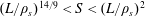
(2.9) $$\begin{eqnarray}(L/\unicode[STIX]{x1D70C}_{s})^{2}\gg S\gg (L/\unicode[STIX]{x1D70C}_{s})^{8/5}.\end{eqnarray}$$

An alternative current sheet profile worth considering – and the one we will make use of in this paper – is that of a sinusoidal-like magnetic field, $B_{y}(x)=B_{0}\sin (x/a)$ , for which $\unicode[STIX]{x1D6E5}^{\prime }\unicode[STIX]{x1D6FF}_{\text{SP}}\sim 1/(k\unicode[STIX]{x1D6FF}_{\text{SP}})^{2}$ . For small $\unicode[STIX]{x1D6E5}^{\prime }$ , we obtain,

(2.10) $$\begin{eqnarray}\displaystyle & \unicode[STIX]{x1D6FE}L/V_{A}\sim (\unicode[STIX]{x1D70C}_{s}/L)^{2/3}(kL)^{-2/3}S, & \displaystyle\end{eqnarray}$$

(2.11) $$\begin{eqnarray}\displaystyle & \unicode[STIX]{x1D6FF}_{\text{in}}\sim (\unicode[STIX]{x1D70C}_{s}/L)^{1/6}(kL)^{-2/3}S^{-1/4}, & \displaystyle\end{eqnarray}$$

valid if $kL\gg (\unicode[STIX]{x1D70C}_{s}/L)^{1/16}S^{15/32}$ . For large $\unicode[STIX]{x1D6E5}^{\prime }$ , the scaling for $\unicode[STIX]{x1D6FE}L/V_{A}$ is same as in (2.4), as there is no explicit dependence on  $\unicode[STIX]{x1D6E5}^{\prime }$ . The fastest growing mode is therefore characterized by

(2.12) $$\begin{eqnarray}\displaystyle & \unicode[STIX]{x1D6FE}_{\text{max}}L/V_{A}\sim (\unicode[STIX]{x1D70C}_{s}/L)^{5/8}S^{11/16}, & \displaystyle\end{eqnarray}$$

(2.13) $$\begin{eqnarray}\displaystyle & k_{\text{max}}L\sim (\unicode[STIX]{x1D70C}_{s}/L)^{1/16}S^{15/32}, & \displaystyle\end{eqnarray}$$

(2.14) $$\begin{eqnarray}\displaystyle & \unicode[STIX]{x1D6FF}_{\text{in}}/L\sim (\unicode[STIX]{x1D70C}_{s}/L)^{1/8}S^{-9/16}. & \displaystyle\end{eqnarray}$$

Figure 1 illustrates both limits of the dispersion relation, and their intersection, for two different combinations of the two relevant parameters, $S$ and $L/\unicode[STIX]{x1D70C}_{s}$ . In the Appendix we recover these scalings via direct numerical simulation, confirming both their validity and the ability of the code Viriato (Loureiro et al. Reference Loureiro, Dorland, Fazendeiro, Kanekar, Mallet, Vilelas and Zocco2016), which we will employ in this paper (see §§ 3 and 4), to recover them.

Figure 1. Dispersion relation for the semi-collisional plasmoid instability for two different combinations of the relevant parameters: $(S,L/\unicode[STIX]{x1D70C}_{s})=(1000,35)$ (red lines) and $(S,L/\unicode[STIX]{x1D70C}_{s})=(10^{6},4000)$ (blue lines). Solid lines represent the case of $\unicode[STIX]{x1D6E5}^{\prime }\unicode[STIX]{x1D6FF}_{\text{in}}\ll 1$ (2.11), whereas dashed lines are for the case of $\unicode[STIX]{x1D6E5}^{\prime }\unicode[STIX]{x1D6FF}_{\text{in}}\gg 1$ (2.4). Respectively, these lines are only valid to the right, or to the left, of their intersection. Their point of intersection provides an estimate of the most unstable wavenumber and corresponding growth rate.

In this case of a sinusoidal-like current sheet profile, equation (2.9) is replaced by:

(2.15) $$\begin{eqnarray}(L/\unicode[STIX]{x1D70C}_{s})^{2}\gg S\gg (L/\unicode[STIX]{x1D70C}_{s})^{14/9}.\end{eqnarray}$$

The lower bound here has only a slightly smaller exponent than (and is in practice difficult to discern from) the Harris-like case of (2.9).

Equations (2.9) and (2.15) lead to the interesting suggestion that this particular version of the plasmoid instability can be obtained at relatively low values of  $S$ , provided that the system (the current sheet length  $L$ , to be precise) is not too large compared with  $\unicode[STIX]{x1D70C}_{s}$ . In other words, the lower bound of $S\sim 10^{4}$ that pertains to the MHD version of the plasmoid instability (Biskamp Reference Biskamp1986; Loureiro et al. Reference Loureiro, Cowley, Dorland, Haines and Schekochihin2005; Samtaney et al. Reference Samtaney, Loureiro, Uzdensky, Schekochihin and Cowley2009; Baty Reference Baty2014) is replaced by a function in the semi-collisional regime, $(L/\unicode[STIX]{x1D70C}_{s})^{14/9}$ , or $(L/\unicode[STIX]{x1D70C}_{s})^{8/5}$ , as appropriate. This growth of plasmoids at low $S$ is possible in the semi-collisional regime due to the presence of the $\unicode[STIX]{x1D70C}_{s}$ scale, which is unavailable in MHD. The tearing calculation in this regime has to account for nested boundary layers instead of a single one: this introduces an extra parameter in the problem and makes the critical Lundquist number (derived from the requirement that the condition for semi-collisional regime, $\unicode[STIX]{x1D6FF}_{\text{SP}}>\unicode[STIX]{x1D70C}_{s}>\unicode[STIX]{x1D6FF}_{\text{in}}$ be satisfied) become dependent on this new parameter.

From both the experimental and the numerical points of view, this feature of low critical Lundquist number is a significant advantage. In particular, this regime should be available to reconnection experiments such as the magnetic reconnection experiment (MRX) (Yamada et al. Reference Yamada, Ji, Hsu, Carter, Kulsrud, Bretz, Jobes, Ono and Perkins1997), terrestrial reconnection experiment (TREX) (Olson et al. Reference Olson, Egedal, Greess, Myers, Clark, Endrizzi, Flanagan, Milhone, Peterson and Wallace2016), facility for laboratory reconnection experiments (FLARE) (Ji & Daughton Reference Ji and Daughton2011) and the mega ampere generator for plasma implosion experiments (Magpie) (Hare et al. Reference Hare, Lebedev, Suttle, Loureiro, Ciardi, Burdiak, Chittenden, Clayson, Eardley and Garcia2017a ,Reference Hare, Suttle, Lebedev, Loureiro, Ciardi, Burdiak, Chittenden, Clayson, Garcia and Niasse b , Reference Hare, Suttle, Lebedev, Loureiro, Ciardi, Chittenden, Clayson, Eardley, Garcia and Halliday2018). Indeed, as we mention above, it is tempting to attribute recent reports of experimental plasmoid observation (Dorfman et al. Reference Dorfman, Ji, Yamada, Yoo, Lawrence, Myers and Tharp2013; Jara-Almonte et al. Reference Jara-Almonte, Ji, Yamada, Yoo and Fox2016; Hare et al. Reference Hare, Lebedev, Suttle, Loureiro, Ciardi, Burdiak, Chittenden, Clayson, Eardley and Garcia2017a ,Reference Hare, Suttle, Lebedev, Loureiro, Ciardi, Burdiak, Chittenden, Clayson, Garcia and Niasse b , Reference Hare, Suttle, Lebedev, Loureiro, Ciardi, Chittenden, Clayson, Eardley, Garcia and Halliday2018) to this version of the plasmoid instability – or to its $\unicode[STIX]{x1D6FD}\sim 1$ analogue (Baalrud et al. Reference Baalrud, Bhattacharjee, Huang and Germaschewski2011) ( $\unicode[STIX]{x1D6FD}$  is the ratio of the plasma pressure to the magnetic pressure). In the weak guide field or $\unicode[STIX]{x1D6FD}\sim 1$ case, the relevant scale is the ion-inertial scale $d_{i}$ (instead of  $\unicode[STIX]{x1D70C}_{s}$ ), and the same feature of scale-dependent critical Lundquist number is expected to hold.

Despite these speculations and conjectures, the existence of this regime of the plasmoid instability has not been confirmed via direct numerical simulations, and indeed there are a couple of issues that may raise suspicion. In particular, we note that all of the scalings above are predicated on there being an asymptotic separation between the scales involved, namely $\unicode[STIX]{x1D6FF}_{\text{SP}}\gg \unicode[STIX]{x1D70C}_{s}\gg \unicode[STIX]{x1D6FF}_{\text{in}}$ .Footnote ⁴ As the Lundquist number is made smaller, this scale separation is inevitably lost, and thus the claim that the semi-collisional plasmoid instability may be obtainable at the relatively low values of $S$ and $L/\unicode[STIX]{x1D70C}_{s}$ that are within the reach of existing experiments needs careful numerical validation.

An additional concern of significant relevance is that of whether the Sweet–Parker sheet that is assumed as the background for the instability derived here is realizable. As has been pointed out (Loureiro et al. Reference Loureiro, Schekochihin and Cowley2007; Pucci & Velli Reference Pucci and Velli2014; Uzdensky & Loureiro Reference Uzdensky and Loureiro2016), the existence of a super-Alfvénic instability whose growth rate diverges as $S\rightarrow \infty$ indicates that the equilibrium that it arises from, may never form in the first place. We think this claim is pertinent at high values of the Lundquist number. However, in the opposite limit of relatively low $S$ with which we are mostly concerned here, where the instability is only mildly super-Alfvénic, a Sweet–Parker sheet may still form and beget the instability.

This paper aims to answer these questions by means of direct numerical simulations of a reconnecting system where the current sheet is not prescribed, but rather allowed to form self-consistently.

3 The model

The weak collisionality of a large number of reconnecting environments demands the use of a kinetic description. In the most general case, one is forced to adopt a first-principles formalism (such as particle-in-cell, or the six-dimensional (6-D) Vlasov (or Boltzmann) equation), with its inherent analytical and numerical complexity. In many situations, however, a strong component of the magnetic field is present that is perpendicular to the reconnection plane. This guide field offers an opportunity for significant simplification: the 5-D gyrokinetic formalism (Frieman & Chen Reference Frieman and Chen1982; Howes et al. Reference Howes, Cowley, Dorland, Hammett, Quataert and Schekochihin2006).

Further simplification is possible if, in addition, one considers plasmas such that the electron $\unicode[STIX]{x1D6FD}$ is sufficiently low to be comparable to the electron-to-ion mass ratio ( $m_{e}/m_{i}$ ); a case in point is the solar corona, as mentioned earlier in § 2. Leveraging on these assumptions (strong guide field and low $\unicode[STIX]{x1D6FD}$ ), a reduced-gyrokinetic formalism was recently derived (dubbed the ‘kinetic reduced electron heating model’, or KREHM) (Zocco & Schekochihin Reference Zocco and Schekochihin2011). One of its appealing features is that the phase space is reduced further to four dimensions (position vector and velocity in the guide-field direction only), thus rendering computations, and even analytic theory, significantly more manageable than fully kinetic approaches.

In this work, we use the KREHM equations to investigate the plasmoid instability in the semi-collisional regime. We will restrict our numerical investigations to the two spatial dimensions comprising the reconnection plane, $(x,y)$ . With this restriction, the KREHM equations become:

(3.1) $$\begin{eqnarray}\displaystyle & \!\displaystyle \frac{1}{n_{0e}}\frac{\text{d}\unicode[STIX]{x1D6FF}n_{e}}{\text{d}t}=\frac{1}{B_{0}}\left\{A_{\Vert },\frac{e}{cm_{e}}d_{e}^{2}\unicode[STIX]{x1D6FB}_{\bot }^{2}A_{\Vert }\right\}\!,\qquad & \displaystyle\end{eqnarray}$$

(3.2) $$\begin{eqnarray}\displaystyle & \!\displaystyle \frac{\text{d}}{\text{d}t}(A_{\Vert }-d_{e}^{2}\unicode[STIX]{x1D6FB}_{\bot }^{2}A_{\Vert })=\unicode[STIX]{x1D702}\unicode[STIX]{x1D6FB}_{\bot }^{2}A_{\Vert }-\frac{cT_{0e}}{eB_{0}}\left\{A_{\Vert },\left(\frac{\unicode[STIX]{x1D6FF}n_{e}}{n_{0e}}+\frac{\unicode[STIX]{x1D6FF}T_{\Vert e}}{T_{0e}}\right)\!\right\}\!,\qquad & \displaystyle\end{eqnarray}$$

(3.3) $$\begin{eqnarray}\displaystyle & \!\displaystyle \frac{\text{d}g_{e}}{\text{d}t}-\frac{v_{\Vert }}{B_{0}}\left\{A_{\Vert },\left(\!g_{e}-\frac{\unicode[STIX]{x1D6FF}T_{\Vert e}}{T_{0e}}F_{0e}\right)\!\right\}=C[g_{e}]-\left(\!1-\frac{2v_{\Vert }^{2}}{v_{\text{the}}^{2}}\right)\frac{F_{0e}}{B_{0}}\left\{A_{\Vert },\frac{e}{cm_{e}}d_{e}^{2}\unicode[STIX]{x1D6FB}_{\bot }^{2}A_{\Vert }\right\}\!,\qquad & \displaystyle\end{eqnarray}$$

where

(3.4) $$\begin{eqnarray}\frac{\text{d}}{\text{d}t}=\frac{\unicode[STIX]{x2202}}{\unicode[STIX]{x2202}t}+\frac{c}{B_{0}}\{\unicode[STIX]{x1D719},\ldots \}.\end{eqnarray}$$

Here, $\unicode[STIX]{x1D719}$ is electrostatic potential and $\{\ldots \}$ denotes the Poisson bracket, defined for any two fields $P$ , $Q$ as $\{P,Q\}=\unicode[STIX]{x2202}_{x}P\unicode[STIX]{x2202}_{y}Q-\unicode[STIX]{x2202}_{y}P\unicode[STIX]{x2202}_{x}Q$ .

Equations (3.1) and (3.2) evolve the zeroth and first moments of the perturbed electron distribution function, $\unicode[STIX]{x1D6FF}f_{e}$ . The zeroth moment is the electron density perturbation, $\unicode[STIX]{x1D6FF}n_{e}$ . The first moment is the parallel electron flow, $u_{\Vert e}$ , and is related to the parallel component of the magnetic vector potential $A_{\Vert }$ by $u_{\Vert e}=(e/cm_{e})d_{e}^{2}\unicode[STIX]{x1D6FB}_{\bot }^{2}A_{\Vert }$ . The perturbed electron distribution function is given by

(3.5) $$\begin{eqnarray}\unicode[STIX]{x1D6FF}f_{e}=g_{e}+(\unicode[STIX]{x1D6FF}n_{e}/n_{0e}+2v_{\Vert }u_{\Vert e}/v_{\text{the}}^{2})F_{0e},\end{eqnarray}$$

where $F_{0e}=n_{0e}/(\unicode[STIX]{x03C0}/v_{\text{the}}^{2})^{3/2}\exp [-(v_{\Vert }^{2}+v_{\bot }^{2})/v_{\text{the}}^{2}]$ is the Maxwellian equilibrium, and $v_{\Vert }$ and $v_{\bot }$ are, respectively, the velocity coordinates parallel and perpendicular to the guide-field direction. The electron thermal speed is $v_{\text{the}}=\sqrt{2T_{0e}/m_{e}}$ , with $e$ the electron charge, and $m_{e}$ its mass. Note that this is a $\unicode[STIX]{x1D6FF}f$ formulation, so any fluctuating quantity is necessarily much smaller than the equilibrium quantity.

The quantity $g_{e}$ is dubbed the reduced electron distribution function; its evolution is given by (3.3). It contains all the moments of $\unicode[STIX]{x1D6FF}f_{e}$ higher than $\unicode[STIX]{x1D6FF}n_{e}$ and $u_{\Vert e}$ . For example, parallel temperature fluctuations (second-order moment) are given by $\unicode[STIX]{x1D6FF}T_{\Vert e}/T_{0e}=(1/n_{0e})\int \,\text{d}^{3}\boldsymbol{v}(2v_{\Vert }^{2}/v_{\text{the}}^{2})g_{e}$ . On the right-hand side, $C[g_{e}]$ denotes the collision operator, and the second term represents what survives of the so-called ‘gyrokinetic potential’ in this expansion.

The background magnetic guide field is $B_{0}$ ; and $n_{0e}$ , $T_{0e}$ are the background electron density and temperature, respectively. Other symbols introduced above are the electron skin depth, $d_{e}=c/\unicode[STIX]{x1D714}_{\text{pe}}$ , with $\unicode[STIX]{x1D714}_{\text{pe}}=\sqrt{4\unicode[STIX]{x03C0}n_{0e}\text{e}^{2}/m_{e}}$ the electron plasma frequency.

The perturbed electron density, $\unicode[STIX]{x1D6FF}n_{e}$ , and the electrostatic potential are related via the gyrokinetic Poisson law,

(3.6) $$\begin{eqnarray}\frac{\unicode[STIX]{x1D6FF}n_{e}}{n_{0e}}=\frac{1}{\unicode[STIX]{x1D70F}}(\hat{\unicode[STIX]{x1D6E4}}_{0}-1)\frac{\text{e}\unicode[STIX]{x1D719}}{T_{0e}},\end{eqnarray}$$

where, $\unicode[STIX]{x1D70F}=T_{0i}/T_{0e}$ is the ion to electron background temperature ratio, and $\hat{\unicode[STIX]{x1D6E4}}_{0}$ is a real space operator whose Fourier transform is $\unicode[STIX]{x1D6E4}_{0}(\unicode[STIX]{x1D6FC})=I_{0}(\unicode[STIX]{x1D6FC})\text{e}^{-\unicode[STIX]{x1D6FC}}$ , with $I_{0}$ the modified Bessel function of zeroth order and $\unicode[STIX]{x1D6FC}=k_{\bot }^{2}{\unicode[STIX]{x1D70C}_{i}}^{2}/2$ , with $\unicode[STIX]{x1D70C}_{i}=v_{\text{thi}}/\unicode[STIX]{x1D6FA}_{i}$ the ion Larmor radius, $v_{\text{thi}}=\sqrt{2T_{0i}/m_{i}}$ the ion thermal velocity and $\unicode[STIX]{x1D6FA}_{i}=|\text{e}|B_{0}/m_{i}c$ the ion gyro frequency.

To make contact with a more familiar set of equations, note that, in the fluid limit ( $d_{e},\unicode[STIX]{x1D70C}_{i},\unicode[STIX]{x1D70C}_{s}\rightarrow 0$ ), equations (3.1) and (3.2) decouple from (3.3) and reduce to the momentum and induction equations of reduced MHD. However, when kinetic effects are retained, Ohm’s law couples to the kinetic equation (3.3) via parallel electron temperature fluctuations.

Observe that (3.3) does not explicitly depend on $v_{\bot }$ . Provided that one chooses a collision operator which is itself also independent of  $v_{\bot }$ , this coordinate can be integrated out, yielding a reduced electron distribution function that is effectively four-dimensional only, $g_{e}=g_{e}(x,y,z,v_{\Vert },t)$ . One model collision operator that exhibits this property is the Lenard–Bernstein operator (Lenard & Bernstein Reference Lenard and Bernstein1958), modified to conserve the pertinent quantities (Zocco & Schekochihin Reference Zocco and Schekochihin2011). Then (3.3) can be more conveniently solved in terms of its expansion in Hermite polynomials:

(3.7) $$\begin{eqnarray}g_{e}(x,y,z,v_{\Vert },t)=\mathop{\sum }_{m=2}^{\infty }\frac{1}{2^{m}m!}H_{m}(v_{\Vert }/v_{\text{the}})g_{m}(x,y,z,t)F_{0e}(v_{\Vert }),\end{eqnarray}$$

where $H_{m}$ denotes the Hermite polynomial of order $m$ and $g_{m}$ is its coefficient. Inserting this expansion into (3.3) yields a coupled set of fluid-like equations for the coefficients of the Hermite polynomials, where by construction $g_{0}=g_{1}=0$ , and for $m\geqslant 2$ we have

(3.8) $$\begin{eqnarray}\displaystyle & & \displaystyle \frac{\text{d}g_{m}}{\text{d}t}-\frac{v_{\text{the}}}{B_{0}}\left(\sqrt{\frac{m+1}{2}}\{A_{\Vert },g_{m+1}\}+\sqrt{\frac{m}{2}}\{A_{\Vert },g_{m-1}\}\right)\nonumber\\ \displaystyle & & \displaystyle \quad =\frac{\sqrt{2}\unicode[STIX]{x1D6FF}_{m,2}}{B_{0}}\left\{A_{\Vert },\frac{e}{cm_{e}}d_{e}^{2}\unicode[STIX]{x1D6FB}_{\bot }^{2}A_{\Vert }\right\}-\unicode[STIX]{x1D708}_{\text{ei}}(mg_{m}-2\unicode[STIX]{x1D6FF}_{m,2}g_{2}),\end{eqnarray}$$

where $\unicode[STIX]{x1D708}_{\text{ei}}$ is the electron–ion collision frequency, $\unicode[STIX]{x1D708}_{\text{ei}}=\unicode[STIX]{x1D702}/d_{e}^{2}$ . The kinetic equations solved by means of Hermite expansion requires a closure. A way to close the set of equations is to demand that at some $m=M$ , the collision term becomes significant such that $g_{M+1}/g_{M}\ll 1$ . This constraint will truncate the kinetic equations at $g_{M}$ as $g_{M+1}$ can be written in terms of $g_{M}$ (Zocco & Schekochihin Reference Zocco and Schekochihin2011; Zocco et al. Reference Zocco, Loureiro, Dickinson, Numata and Roach2015; Loureiro et al. Reference Loureiro, Dorland, Fazendeiro, Kanekar, Mallet, Vilelas and Zocco2016; White & Hazeltine Reference White and Hazeltine2017). This type of closure also recovers the semi-collisional limit exactly.

4 Numerical set-up

Equations (3.1), (3.2), (3.6) and (3.8) are solved numerically on a two-dimensional grid of size $L_{x}\times L_{y}$ , using the pseudo-spectral code Viriato (Loureiro et al. Reference Loureiro, Dorland, Fazendeiro, Kanekar, Mallet, Vilelas and Zocco2016). Periodic boundary conditions are employed in both directions. The numerical configuration is akin to that employed in Loureiro et al. (Reference Loureiro, Cowley, Dorland, Haines and Schekochihin2005) and, as we will show, is such that one can self-consistently obtain an SP current sheet whose stability to plasmoid formation can then be studied. Specifically, the input parameters can be specified in a way as to lead to the dynamic formation of a SP current sheet that meets the conditions of the semi-collisional regime that we have discussed earlier.

The initial equilibrium is $A_{\Vert }(x,y,t=0)=A_{\Vert 0}/\cosh ^{2}(x)$ , where $A_{\Vert 0}=3\sqrt{3}/4$ , such that the maximum of the reconnecting field, $B_{y}=\text{d}A_{\Vert }/\text{d}x$ , is $B_{y,\text{max}}=1$ . This equilibrium is destabilized with a small amplitude (linear) perturbation which seeds the fastest growing tearing mode; in all simulations, this is the longest wavelength mode that fits in the simulation box. Once in the nonlinear stage, the tearing mode undergoes $X$ -point collapse (Waelbroeck Reference Waelbroeck1989; Loureiro et al. Reference Loureiro, Cowley, Dorland, Haines and Schekochihin2005), and a current sheet forms which is consistent with the SP scaling (as we shall confirm). The plasmoid instability is then triggered, or not, depending on the values of $S$ and $\unicode[STIX]{x1D70C}_{s}$ specified in the simulation.

The length of the SP current sheet can be varied by changing the instability parameter, $\unicode[STIX]{x1D6E5}^{\prime }(k)$ , pertaining to the initial tearing mode (Loureiro et al. Reference Loureiro, Cowley, Dorland, Haines and Schekochihin2005). In practice, this is achieved by changing the length of the box in the outflow direction,  $L_{y}$ .

The resolution of a simulation in the inflow ( $x$ ) direction is set by the size of the inner boundary layer that is expected to arise due to the plasmoid instability, estimated using (2.8). The resolution demands in the outflow ( $y$ ) direction are less stringent, and are determined on a ad hoc basis.

An additional constraint on our runs is that the electron inertia play no role. This is insured by setting it to be smaller than the resolution for any given simulation. Therefore, in all runs, the frozen-flux constraint is broken by resistivity. Note that no hyper-resistivity (or hyper-viscosity) is used in these runs, ensuring that the actual Lundquist number in the simulations is determined by the resistivity that we specify. The simulations also employ a finite viscosity, set equal to the magnetic diffusivity.

A final choice has to do with the number of Hermite polynomials to keep in the simulations. For all runs reported here, the highest-order polynomial is $M=4$ – this ought to be sufficient given the relatively high collisionality of our simulations (and indeed we find that in all our runs resistivity is the dominant energy dissipation channel). To check convergence, we performed one test using instead $M=10$ , and observed that in the spectrum of $|g_{m}|^{2}/2$ , the energy at $m>3$ –4, is lower than that at $m=2$ by orders of magnitude, indicating that the power transferred to the Hermite polynomials of higher order is not significant. In all runs, the convergence of the Hermite representation is accelerated by the use of a hyper-collision operator (see Loureiro et al. (Reference Loureiro, Dorland, Fazendeiro, Kanekar, Mallet, Vilelas and Zocco2016) for details).

6 Discussions and conclusions

In this paper, we have investigated, analytically and numerically, the semi-collisional regime of the plasmoid instability – an extension to a Sweet–Parker sheet of the semi-collisional tearing mode (Drake & Lee Reference Drake and Lee1977; Cowley, Kulsrud & Hahm Reference Cowley, Kulsrud and Hahm1986; Zocco & Schekochihin Reference Zocco and Schekochihin2011). We employ a reduced kinetic formalism obtainable from the gyrokinetic formalism via asymptotic expansion in low plasma $\unicode[STIX]{x1D6FD}$ (Zocco & Schekochihin Reference Zocco and Schekochihin2011). The simulations are carried out with the code Viriato (Loureiro et al. Reference Loureiro, Dorland, Fazendeiro, Kanekar, Mallet, Vilelas and Zocco2016). This regime is analytically predicted to occupy a significant sliver of the reconnection phase diagram defined by a lower bound $S>(L/\unicode[STIX]{x1D70C}_{s})^{14/9}$ and an upper bound $S<(L/\unicode[STIX]{x1D70C}_{s})^{2}$ . Our numerical simulations show that these bounds are remarkably robust: runs which fall within these two bounds yield the plasmoid instability, and vice versa. The instability arises at much lower values of the Lundquist numbers than the MHD analogue; as low as $S\sim 250$ . We are limited in our exploration of even lower values of $S$ by our simulation set-up. Thus, we do not rule out the formation of plasmoids for $S<250$ in less constrained systems; indeed, we speculate that this regime could also potentially explain formation of plasmoids in recent reconnection experiments (Jara-Almonte et al. Reference Jara-Almonte, Ji, Yamada, Yoo and Fox2016; Hare et al. Reference Hare, Lebedev, Suttle, Loureiro, Ciardi, Burdiak, Chittenden, Clayson, Eardley and Garcia2017a ,Reference Hare, Suttle, Lebedev, Loureiro, Ciardi, Burdiak, Chittenden, Clayson, Garcia and Niasse b , Reference Hare, Suttle, Lebedev, Loureiro, Ciardi, Chittenden, Clayson, Eardley, Garcia and Halliday2018). In Magpie, for example, we find from table I in Hare et al. (Reference Hare, Suttle, Lebedev, Loureiro, Ciardi, Chittenden, Clayson, Eardley, Garcia and Halliday2018) that $S\approx 120$ and $L/d_{i}\approx 18$ . If we were to consider the relevant kinetic scale to be $d_{i}$ instead of  $\unicode[STIX]{x1D70C}_{s}$ , then the value of these parameters ( $S$ and $L/d_{i}$ ) satisfy the condition for the semi-collisional regime and fall within its bounds. Note that in the collisionless (or weakly collisional) regime, plasmoids arise only when $L/\unicode[STIX]{x1D70C}_{s}$ is larger than a value of about ${\sim}50$ (an empirical value seen in simulations) (Ji & Daughton Reference Ji and Daughton2011), whereas the semi-collisional regime seems to offer no hard lower bound. Further, with the validation of the existence of this regime, the reconnection phase diagram (figure 1 in Ji & Daughton Reference Ji and Daughton2011) would be modified. The lower bound of this regime, governed by either $S=(L/\unicode[STIX]{x1D70C}_{s})^{14/9}$ or $S=(L/\unicode[STIX]{x1D70C}_{s})^{8/5}$ would now cut across the two lines – one line representing the critical Lundquist number for MHD plasmoid instability ( $S=S_{c}$ ) and then a second line representing the lower bound of the multiple $X$ -line hybrid regime ( $S=L\sqrt{S_{c}}/2\unicode[STIX]{x1D70C}_{s}$ ).

The numerical experiments reported here are limited in that the amount of flux to reconnect is finite, and the simulation box is periodic. As such, (statistical) steady state reconnection cannot be attained, thereby preventing us from numerically answering the important question of what the reconnection rate is in the semi-collisional plasmoid regime. However, theoretically we may expect the following. In the phase-space diagram of figure 3, assume that the initial system, with a certain $S$ , $L$ and  $\unicode[STIX]{x1D70C}_{s}$ , is in the semi-collisional regime. As the plasmoid instability unfolds, we expect that smaller, interplasmoid current sheets will arise. These will necessarily have a smaller length, $L^{\prime }\sim L/N$ , where $N$ is the number of primary plasmoids. Each of these interplasmoid current sheets now defines a reconnecting site which can be located in the reconnection phase diagram. Since $\unicode[STIX]{x1D70C}_{s}$ and $\unicode[STIX]{x1D702}$ are fixed, and assuming that $V_{A}$ is the same in these daughter sheets, the only parameter that has changed is the length, from $L$ to  $L^{\prime }$ . This means a diagonal displacement in the direction of smaller $L/\unicode[STIX]{x1D70C}_{s}$ from the initial point in that diagram; the slope of that diagonal is 1, because both axes are linearly proportional to  $L$ . If the new position in this diagram remains in the semi-collisional regime, each interplasmoid current sheet is still unstable to the semi-collisional plasmoid instability. The process then repeats (i.e. the plasmoid hierarchy unfolds further) until arriving at an interplasmoid current sheet which is now short enough to be outside of the semi-collisional bounds. Inevitably, therefore, this lands the system to the left of the $S\sim (L/\unicode[STIX]{x1D70C}_{s})^{2}$ bound, i.e. the collisionless regime, where the expected reconnection rate is ${\sim}0.1\unicode[STIX]{x1D70F}_{A}^{-1}$ . Defining $\unicode[STIX]{x1D706}_{c}=(L_{c}/\unicode[STIX]{x1D70C}_{s})$ as an empirical scale separating the single from the multiple $X$ -line collisionless regimes (numerically observed to be ${\sim}50$ ), we conclude that the system finally lands in either the multiple, or single, $X$ -line collisionless regime depending on whether it is initially above or below the diagonal line $S\sim \unicode[STIX]{x1D706}_{c}(L/\unicode[STIX]{x1D70C}_{s})$ , (which intersects the line $S\sim (L/\unicode[STIX]{x1D70C}_{s})^{2}$ at $(L/\unicode[STIX]{x1D70C}_{s})=\unicode[STIX]{x1D706}_{c}$ ) in the reconnection phase space diagram.

Finally, let us outline some general arguments for the case when, unlike our simulations, the global Lundquist number of the system is so large that a Sweet–Parker current sheet may not be able to form dynamically. Consider then a forming current sheet, and assume for simplicity that the characteristic time at which it is forming is Alfvénic, $\unicode[STIX]{x1D70F}_{A}=L/V_{A}$ . At any given moment of time, we parameterize the forming current sheet aspect ratio as $a/L=S^{-\unicode[STIX]{x1D6FC}}$ (Pucci & Velli Reference Pucci and Velli2014), where $a$ is the current sheet width, and $\unicode[STIX]{x1D6FC}$ is a number such that $0<\unicode[STIX]{x1D6FC}<1/2$ , with $\unicode[STIX]{x1D6FC}=1/2$ representing a Sweet–Parker sheet (which the system presumably never gets to).

Using (2.6) (for a Harris-type sheet) we see that the growth rate of the most unstable semi-collisional mode exceeds the current sheet formation rate (Alfvénic) when

(6.1) $$\begin{eqnarray}\unicode[STIX]{x1D6FE}_{\text{max}}\unicode[STIX]{x1D70F}_{A}\sim (\unicode[STIX]{x1D70C}_{s}/L)^{2/3}S^{-1/3+2\unicode[STIX]{x1D6FC}}\gtrsim 1.\end{eqnarray}$$

This expression constrains the relationship between $S$ and $L/\unicode[STIX]{x1D70C}_{s}$ , for any value of  $\unicode[STIX]{x1D6FC}$ , to attain Alfvénic growth at that value of  $\unicode[STIX]{x1D6FC}$ . In addition, we must further require that this mode (the most unstable semi-collisional mode) is indeed in the semi-collisional regime, i.e. $\unicode[STIX]{x1D6FF}_{\text{in},\text{max}}^{SC}<\unicode[STIX]{x1D70C}_{s}$ . This leads to,

(6.2) $$\begin{eqnarray}(\unicode[STIX]{x1D70C}_{s}/L)^{1/9}S^{-(2\unicode[STIX]{x1D6FC}/3)-2/9}<\unicode[STIX]{x1D70C}_{s}/L.\end{eqnarray}$$

These two expressions intersect when $\unicode[STIX]{x1D6FC}=1/3$ . That is, if $\unicode[STIX]{x1D6FC}<1/3$ , the relationship that $S$ and $L/\unicode[STIX]{x1D70C}_{s}$ must satisfy to yield Alfvénic growth is given by (6.1); if instead $\unicode[STIX]{x1D6FC}>1/3$ , then it is sufficient to satisfy (6.2) to attain Alfvénic growth.Footnote ⁶

A detailed analysis of all different possibilities that are encountered as $\unicode[STIX]{x1D6FC}$ increases is beyond the scope of this paper and will be left to future work. Generally, for $\unicode[STIX]{x1D6FC}<1/3$ , the condition for the fastest semi-collisional mode to become faster than Alfvénic becomes progressively less demanding on  $S$ . Consider the particularly interesting case where $\unicode[STIX]{x1D6FC}$ reaches the value of $1/3$ . At this value, we must have $S>(L/\unicode[STIX]{x1D70C}_{s})^{2}$ for the semi-collisional mode to both exist and be super-Alfvénic. Remarkably, $\unicode[STIX]{x1D6FC}=1/3$ is the value at which the fastest growing MHD mode becomes Alfvénic (Pucci & Velli Reference Pucci and Velli2014). The condition for that mode to indeed be in the MHD regime is, unsurprisingly, just the reverse of the above, $S<(L/\unicode[STIX]{x1D70C}_{s})^{2}$ . So, in this case ( $\unicode[STIX]{x1D6FC}=1/3$ ), the outcome is particularly simple: if $S>(L/\unicode[STIX]{x1D70C}_{s})^{2}$ the forming sheet would be disrupted by a semi-collisional mode, and one might expect the reconnection rate to ensue to be $0.1\unicode[STIX]{x1D70F}_{A}^{-1}$ as discussed above; if, instead $S<(L/\unicode[STIX]{x1D70C}_{s})^{2}$ then the sheet would be disrupted by an MHD mode, and the reconnection rate would presumably be $S_{c}^{-1/2}\unicode[STIX]{x1D70F}_{A}^{-1}\sim 0.01\unicode[STIX]{x1D70F}_{A}^{-1}$ (unless a transition to the semi-collisional regime occurs during the plasmoid cascade – see footnote 4 on page 5). For example, in the solar corona, where $S\sim 10^{13}$ and $L/\unicode[STIX]{x1D70C}_{s}\sim 10^{7}$ , we see that the MHD mode would win.