2 Physical model

The physical model presented in this work has been developed in a previous paper (Peter et al. Reference Peter, Endler, Rizzato and Serbeto2013). Thus, only the final expressions for the equations are shown.

The wiggler $(\boldsymbol{A}_{w})$ and the laser $(\boldsymbol{A})$ fields are described by their vector potentials fields, respectively

$\unicode[STIX]{x1D714}$ is the frequency of the radiation; $a=a(z)$ is the slowly varying dimensionless amplitude of the laser and $a_{w}$ is the dimensionless undulator parameter; $z$ is the position of the beam; and $\hat{\boldsymbol{e}}$ is the circular polarization vector.

The 1-D FEL dynamics is well described by particle equations for the energy $\unicode[STIX]{x1D6FE}$ and phase $\unicode[STIX]{x1D703}$ ( $=[k+k_{w}]z-\unicode[STIX]{x1D714}t$ ), and the wave equation for the laser amplitude $a(z)$ . These equations form what is called wave–particle system, composed by $2N+2$ equations, where $N$ is the number of particles (in the present paper we considered $1000$ particles for the cold beam case and $5000$ particles for the warm beam case). The equations, shown below, were solved using the LSODE code (Hindmarsh Reference Hindmarsh1980, Reference Hindmarsh and Stepleman1983) and they were normalized in a way that: $t=\unicode[STIX]{x1D714}t$ , $v=v/c$ and $z=v_{p}t=k/(k+k_{w})t$

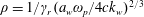
In these equations, $j$ is the index for each particle, while the index $k$ refers to the other particles; the brackets indicate an average over the particle distribution (thus, there is an equation of energy and an equation of phase for each particle); the quantity $\unicode[STIX]{x1D702}$ is the space-charge factor arising from the beam charge, $\unicode[STIX]{x1D702}^{2}={\unicode[STIX]{x1D714}_{p}}^{2}/\unicode[STIX]{x1D714}^{2}$ , with $\unicode[STIX]{x1D714}_{p}=\sqrt{4\unicode[STIX]{x03C0}n_{0}e^{2}/m}$ being the plasma frequency and $n_{0}$ is the average density of particles; the velocity of the ponderomotive potential is represented by $v_{p}=k/(k_{w}+k)=k/k_{p}<1$ ; $\unicode[STIX]{x1D708}$ is the detuning, which is a dimensionless parameter that measures somehow the difference between the ponderomotive potential velocity ( $v_{p}$ ) and the beam velocity ( $v_{p}^{\prime }$ ): $\unicode[STIX]{x1D708}=(v_{p}^{\prime }-v_{p})/v_{p}^{\prime }$ ; and the longitudinal particle velocity is given through the relativistic Lorentz factor definition: ${v_{z}}_{j}=[1-(1-\left|a_{tot}\right|^{2})/{\unicode[STIX]{x1D6FE}_{j}}^{2}]^{1/2}$ , with $\left|a_{tot}\right|^{2}=\left|a_{w}(\exp [\text{i}(k_{w}z)]+\text{c.c.})+(a\,\exp [\text{i}(kz-\unicode[STIX]{x1D714}t)]+\text{c.c.})\right|^{2}$ .

The total energy of the system is conserved while the system evolves. Dividing the energy by a volume and using the Poynting vector is possible to find a relation in which the density of energy is conserved ( $n_{0}\langle \unicode[STIX]{x1D6FE}\rangle mc^{2}+|E|^{2}/4\unicode[STIX]{x03C0}=\unicode[STIX]{x1D716}^{\ast }=\text{const}.$ , where $|E|$ is the modulus of the electric field of the laser) (Bonifacio et al. Reference Bonifacio, Casagrande, Cerchoni, de Salvo Souza, Pierini and Piovella1990). This relation is rewritten in terms of the variables defined in this section as $\unicode[STIX]{x1D702}^{2}\langle \unicode[STIX]{x1D6FE}\rangle +|a|^{2}=\unicode[STIX]{x1D716}$ .

The evolution of the laser amplitude is well described by the models, both for the initially cold and warm beam in the linear regime. Some considerations are made to evaluate the gain (its maximum is measured taking the first peak of the laser amplitude). The gain, $\unicode[STIX]{x1D6E4}$ , is defined with help of a decibel scale as

The theoretical gain given by wave-particle equations is compared to the models prediction in the next sections.

3 Cold beam

The first case analysed in this paper is the initially cold beam case. It implies that at $z=0$ all of the particles of the beam have the same velocity ( $v_{p}^{\prime }$ ) and energy ( $\unicode[STIX]{x1D6FE}_{r}$ ). As shown in a previous work (Peter et al. Reference Peter, Endler, Rizzato and Serbeto2013), the onset of mixing takes place in the phase space when the local electron density, at the position of the onset, goes to infinity. Then, the compressibility factor (which is defined as $C\propto n_{0}/n$ , where $n$ is the local density) goes to zero. This occurs because the distribution of the particles becomes a multi-valued function. A very similar model was recently applied to the case of magnetically focused beams as well (Souza et al. Reference Souza, Endler, Pakter, Rizzato and Nunes2010).

In the model, the complete set of equations, given by equations (2.3)–(2.5), is linearized as in Bonifacio et al. (Reference Bonifacio, Casagrande, Cerchoni, de Salvo Souza, Pierini and Piovella1990). Thus, the linear evolution of the radiation field is obtained through the integration of the following set of equations (where dot indicates time derivation)

where the collective complex variable $X$ represents the fluctuations in the phase ( $X=\langle \text{e}^{-\text{i}\tilde{\unicode[STIX]{x1D703}}_{0}}\unicode[STIX]{x1D6FF}\tilde{\unicode[STIX]{x1D703}}\rangle$ ), while the subscript $0$ refers to the initial condition and $\unicode[STIX]{x1D6FF}\tilde{\unicode[STIX]{x1D703}}=\tilde{\unicode[STIX]{x1D703}}-\tilde{\unicode[STIX]{x1D703}}_{0}$ ; the collective complex variable $Y$ represents the fluctuations in the energy ( $Y=\langle \text{e}^{-\text{i}\tilde{\unicode[STIX]{x1D703}}_{0}}\unicode[STIX]{x1D6FF}\unicode[STIX]{x1D6FE}\rangle$ ) and $\unicode[STIX]{x1D6FF}\unicode[STIX]{x1D6FE}=\unicode[STIX]{x1D6FE}-\unicode[STIX]{x1D6FE}_{0}$ ; $\tilde{a}$ is the transformed complex laser amplitude ( $\tilde{a}\text{e}^{\text{i}\tilde{\unicode[STIX]{x1D703}}}=a\text{e}^{\text{i}\unicode[STIX]{x1D703}}$ ); and, $\tilde{\unicode[STIX]{x1D703}}$ is the transformed phase $(\unicode[STIX]{x1D703}=\tilde{\unicode[STIX]{x1D703}}-\unicode[STIX]{x1D708}z)$ ; the subscript $r$ refers to the resonance condition; in the case of a cold beam ${\dot{Y}}|_{therm}=0$ : this term will be explained later (this term is added due to thermal effects).

With these coupled equations it is possible to generate a third-order polynomial equation to determine the parameters that lead to the maximum growth rate and the instability limits. The linear set of equations also provides the linear growth of the laser amplitude. In Bonifacio et al. (Reference Bonifacio, Casagrande, Cerchoni, de Salvo Souza, Pierini and Piovella1990), for example, the linear growth rate is analysed including space-charge effects.

But the linear set of equations itself is unable to predict the onset of the phase-space mixing. In the model, the nonlinearities of the space-charge effects are introduced due to a connection between the phase and the energy. By exploring this connection, a second-order ordinary differential equation for the phase, which depends on the initial phase, $\tilde{\unicode[STIX]{x1D703}}_{0j}$ , is written as

where $\unicode[STIX]{x1D712}_{1}\equiv a_{w}(1+{a_{w}}^{2})/(2{v_{p}}^{2}(1-\unicode[STIX]{x1D708}){\unicode[STIX]{x1D6FE}_{r}}^{4})$ and $\unicode[STIX]{x1D712}_{2}\equiv \unicode[STIX]{x1D702}^{2}(1+{a_{w}}^{2})/((1-\unicode[STIX]{x1D708}){\unicode[STIX]{x1D6FE}_{r}}^{3})$ .

Deriving (3.4) with respect to $\tilde{\unicode[STIX]{x1D703}_{0}}$ , and defining $\unicode[STIX]{x2202}\tilde{\unicode[STIX]{x1D703}}_{j}/\unicode[STIX]{x2202}\tilde{\unicode[STIX]{x1D703}}_{0}\equiv C$ as the compressibility factor, we obtain an evolution equation that indicates the beginning of the phase mixing (it occurs in the model when the first $\tilde{\unicode[STIX]{x1D703}}_{0}$ satisfies the condition $C\rightarrow 0$ ). The equation of the compressibility evolution is given by

The linear equations combined with (3.4) and (3.5) form our simplified model that can estimate the position $z$ and $\unicode[STIX]{x1D703}$ of the onset of mixing, the saturated amplitude of the laser and the critical value of $\unicode[STIX]{x1D708}$ responsible to separate Compton and Raman regimes (Peter et al. Reference Peter, Endler, Rizzato and Serbeto2013). These equations are solved also using the LSODE code (Hindmarsh Reference Hindmarsh1980, Reference Hindmarsh and Stepleman1983).

In the model, the position $z$ of the onset of mixing is obtained when the first $\tilde{\unicode[STIX]{x1D703}}_{0}$ satisfies the condition $C\rightarrow 0$ : this position is called $z_{0}$ . This point forward, we freeze the collective variables $X$ and $Y$ . Thus, the amplitude $|a|$ oscillates and we take the maximum value of it. This value, obtained through the model, is assumed to estimate the first peak amplitude in the wave–particle simulations.

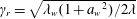
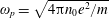
Figure 1. Map $\unicode[STIX]{x1D702}$ versus $\unicode[STIX]{x1D708}$ of the gain $\unicode[STIX]{x1D6E4}$ . The colours indicate the gain, in dB. The black solid lines are from the linear analysis and they delimit the instable region. The dashed line is the curve which maximizes the growth rate. Finally, the indexed filled circles are the points used to compare the model and the full simulations results. The commas appear because the gain depends on a combination between the growth rate and the position $z_{0}$ of the onset of the mixing.

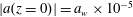
Figure 1 shows a map of the gain for the model, in terms of $\unicode[STIX]{x1D708}$ and $\unicode[STIX]{x1D702}$ . The map was built for $a_{w}=0.5$ , $|a(z=0)|=a_{w}\times 10^{-5}$ and $v_{p}=0.99$ $-$ these values correspond to an initial beam energy of the order of ${\sim}4$  MeV. The black solid lines represent the limits of the instability region, while the dashed line is the maximum growth rate curve obtained from the cubic polynomial of the linear set of equations. The colours indicate the gain and the indexed circles, from $A$ to $D$ , denote the points used to compare the model and the full simulations $-$ and are over the curve of maximum growth rate. The values of the gain vary from $0$ to ${\approx}47$  dB and grow by increasing the value of $\unicode[STIX]{x1D702}$ .

Figure 2. The figure depicts the behaviour of $\unicode[STIX]{x1D6E4}$ versus $\unicode[STIX]{x1D702}$ . The solid line corresponds to the result from wave–particle simulations, while the filled circles are from the model. The indexed points correspond exactly to the ones of figure 1. The pair $\unicode[STIX]{x1D702}$ and $\unicode[STIX]{x1D708}$ is over the maximum growth rate curve. The red curve is the gain considering $P_{sat}=\unicode[STIX]{x1D70C}P_{beam}$ .

In figure 2, the points from $A$ to $D$ of figure 1 are compared. The horizontal axis represents $\unicode[STIX]{x1D702}$ , while the vertical axis shows the gain, $\unicode[STIX]{x1D6E4}$ . The indexed points represent the result from the model, while the solid line is obtained from wave–particle simulations. Until the point $A$ ( $\unicode[STIX]{x1D702}=0.01$ ) the gain is very sensible to the space-charge effects: the gain is increased by three orders of magnitude (from zero to $\unicode[STIX]{x1D6E4}=30$  dB). In this region, the kinetic energy available for the energy conversion increases as $\unicode[STIX]{x1D702}$ increases. The space-charge effects also increase, but the ponderomotive potential mainly drives the dynamics of the particles. This corresponds to the Compton regime (Peter et al. Reference Peter, Endler, Rizzato and Serbeto2013).

After the point $A$ , the gain still grows, but in, according to figure 2, an approximately linear fashion. This occurs because the space-charge effects becomes relevant to the system dynamics. The space-charge effects act against the ponderomotive potential. While the ponderomotive tends to attract the particles (forming micro-bunches), the space charge acts to the contrary. It is typical of Raman or near Raman regimes (Peter et al. Reference Peter, Endler, Rizzato and Serbeto2013).

Moreover, the red curve of figure 2 is obtained from a relation described in McNeil & Thompson (Reference McNeil and Thompson2010), Milton et al. (Reference Milton, Gluskin, Arnold, Benson, Berg, Biedron, Borland, Chae, Dejus and Den Hartog2001), Kim (Reference Kim1986) for an initially cold beam, considering space-charge effects. The relation is given by $P_{sat}=\unicode[STIX]{x1D70C}P_{beam}$ , where $P_{sat}$ is the saturation power of the laser, $P_{beam}$ is the beam power and $\unicode[STIX]{x1D70C}$ is the FEL parameter Bonifacio et al. 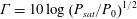(Reference Bonifacio, Casagrande, Cerchoni, de Salvo Souza, Pierini and Piovella1990), while the gain can be written as $\unicode[STIX]{x1D6E4}=10\log \left(P_{sat}/P_{0}\right)^{1/2}$ , where $P_{0}$ is the initial power of the laser. The FEL parameter is written as $\unicode[STIX]{x1D70C}=1/\unicode[STIX]{x1D6FE}_{r}(a_{w}\unicode[STIX]{x1D714}_{p}/4ck_{w})^{2/3}$ . Using the variables transformation proposed in this work, we obtain

Thus, the red curve agrees very well with the simulations and, consequently, with the simplified model given in this work. The simplified model gave values of the gain higher than the wave–particle simulations of the order of a few per cent. This way, the model agrees well with the wave–particle simulations, proving to be a good tool to estimate the amplification of the laser.

4 Warm beam

For a warm beam, at $z=0$ we consider that the velocity of the particles is given by a water bag distribution function, where $\unicode[STIX]{x0394}v_{0}$ is the half-width of the distribution, while the particles distribution in the phase space is spatially homogeneous. The difference, in terms of the wave–particle equations’ integration, consists in a change in the initial conditions of the particles. The evolution of the particles in the phase space occurs in a laminar fashion until nonlinearities begin to dominate the system dynamics. The breakdown of the laminar regime is defined when the lower border of the particle distribution in the phase space becomes a multi-valued function.

Non-relativistic water bag distributions with constant density over the occupied phase space are exactly represented by adiabatic fluid equations (Coffey Reference Coffey1971), while the laminar regime persists. In the model, we consider very small values of velocity spread $-$ in the hydrodynamical regime, i.e. $\unicode[STIX]{x0394}v_{0}<\unicode[STIX]{x1D708}$ . In this limit, we can use the non-relativistic approximation and the connections between widths in velocity, momentum and energy are approximately linear and their interaction is efficient (Marshall Reference Marshall1985; Brau Reference Brau1990). This guarantees that if the density is constant in one phase-space representation, then the density is constant in another.

By exploring the connection between (2.3) and (2.4), identifying a pressure term and the thermal effects over the system through the Vlasov equation and its moments (exactly as in Peter et al. Reference Peter, Endler and Rizzato2014) and using a relation between the pressure and the initial velocity spread for a non-relativistic water bag distribution given in Coffey (Reference Coffey1971) (the relation, although for non-relativistic water bag distribution, is valid for very narrow initial distributions), a linear term that represents the thermal effect in the system is written as

where $D_{\unicode[STIX]{x1D6FE}^{2}}=\unicode[STIX]{x2202}^{2}v/\unicode[STIX]{x2202}\unicode[STIX]{x1D6FE}^{2}$ .

In the presence of an initial spread, a pressure term $\neq 0$ is added to the linear equations. Precisely, (4.1) is replaced in (3.3). The thermal effect acts like the space-charge effect, reducing the linear growth rate. The linear growth rate obtained from this linear set of equations is close to the wave–particle simulations’ growth rate and it is within a range of $6\,\%$ from calculations in the literature (Chakhmachi & Maraghechi Reference Chakhmachi and Maraghechi2009).

The thermal effect must be included in the evolution of the beam element $\tilde{\unicode[STIX]{x1D703}}_{j}$ . We do this by preserving the nonlinearities neglected to generate (4.1). This way, (3.4) is changed, giving place to

where $\unicode[STIX]{x1D6FF}\tilde{\unicode[STIX]{x1D703}}_{j}=\tilde{\unicode[STIX]{x1D703}}_{j}-\tilde{\unicode[STIX]{x1D703}}_{0}$ .

Differently to (3.4), which is an ordinary differential equation, equation (4.2) is a partial differential equation, which is solved numerically through the finite differences method. The laser amplitude in this equation is given by the integration of the linear system, (3.1)–(3.3) and (4.1), and the equation is solved through the partition of the beam into a large number of discrete elements. Differently to the cold case, in the case of a warm beam, the compressibility factor never goes to zero due the presence of the thermal effects (a similar analysis was made by the group for warm magnetically focused beams (Souza et al. Reference Souza, Endler, Rizzato and Pakter2012)). Then, the breakdown of the laminar regime is reached when density discontinuities are established.

The nonlinear model estimates quite well the peak amplitude of the radiation (Peter et al. Reference Peter, Endler and Rizzato2014). If we consider that the breakdown of the laminar regime is located at $z_{b}$ , from this point forward, the collective variables $X$ and $Y$ are frozen. As in the cold case, the laser dynamics, then, becomes oscillatory. The maximum value of these oscillations correspond to the estimated peak of the radiation field.

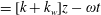
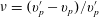
Figure 3 shows the gain, $\unicode[STIX]{x1D6E4}$ against $\unicode[STIX]{x1D702}$ for $v_{p}=0.99$ , $a_{w}=0.5$ and $|a(z=0)|=a_{w}\times 10^{-5}$ and different values of $\unicode[STIX]{x0394}v_{0}$ , always over the curve that maximizes the growth rate. The filled circles are from the model, while the lines are from wave–particle simulations. Each colour corresponds to a different value of $\unicode[STIX]{x0394}v_{0}$ : black is for $\unicode[STIX]{x0394}v_{0}=0.0002$ and red is for $\unicode[STIX]{x0394}v_{0}=0.0008$ .

Figure 3. In this figure is plotted $\unicode[STIX]{x1D6E4}$ versus $\unicode[STIX]{x1D702}$ . The solid line corresponds to the result from the wave–particle simulations, while the filled circles are from the theoretical model. The red (black) ones correspond to $\unicode[STIX]{x0394}v_{0}=0.0008$ ( $\unicode[STIX]{x0394}v_{0}=0.0002$ ). The pair $\unicode[STIX]{x1D702}$ and $\unicode[STIX]{x1D708}$ is over the maximum growth rate curve.

It is possible to see that the gain is diminished as the initial velocity spread increases. The thermal effect act like the space charge, in opposition to the ponderomotive potential. With the increase of the charge in the system, the thermal effects become less important in the dynamics. Thus, the curves tend to bring together as we increase $\unicode[STIX]{x1D702}$ . These results agree with what was shown in the previous work (Peter et al. Reference Peter, Endler and Rizzato2014).

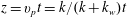
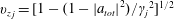
In figure 4, we plot the gain against the initial velocity spread for a fixed, and small, $\unicode[STIX]{x1D702}$ ( $\unicode[STIX]{x1D702}=0.01$ , $a_{w}=0.5$ and $|a(z=0)|=a_{w}\times 10^{-5}$ ). The solid black line was obtained from wave–particle simulations, while the filled circles are from the model. The dashed line is a fit curve of the filled circles.

Figure 4. $\unicode[STIX]{x1D6E4}$ is plotted against $\unicode[STIX]{x0394}v_{0}$ for $v_{p}=0.99$ , $\unicode[STIX]{x1D702}=0.01$ , $a_{w}=0.5$ and 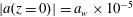$|a(z=0)|=a_{w}\times 10^{-5}$ . The solid line corresponds to the result from the wave–particle simulations, while the filled circles are from the theoretical models. The dashed line is a fit curve for the filled circles. The pair $\unicode[STIX]{x1D702}$ and $\unicode[STIX]{x1D708}$ is over the maximum growth rate curve.

As can be seen in figure 4, the model is more sensitive in relation to $\unicode[STIX]{x0394}v_{0}$ than the wave–particle system. For small values of $\unicode[STIX]{x0394}v_{0}$ , the oscillations of the laser field in the model are greater than the wave–particle simulations. Thus the model tends to overestimate the gain in that region. While for values of $\unicode[STIX]{x0394}v_{0}$ near the limit of the hydrodynamical regime, the model tends to underestimate the gain. This is the effect of the temperature over the model when we freeze the collective variables. The oscillations of the laser field become smaller as we increase $\unicode[STIX]{x0394}v_{0}$ .

Although the difference is of the order of $15\,\%$ for the gain for very small $\unicode[STIX]{x0394}v_{0}$ , the model proved to estimate in a reasonable way the gain obtained from wave–particle simulations and the decreasing tendency of the gain by increasing $\unicode[STIX]{x0394}v_{0}$ .