


1. Introduction
Systematic longevity risk is a looming threat to pension systems worldwide. In contrast to idiosyncratic longevity risk, which is the risk surrounding an individual's actual date of death given known survival probabilities, systematic longevity risk concerns the misestimation of future survival probabilities.Footnote 1 The persistent trend toward improved life expectancy and the increased uncertainty in mortality developments make it clear that systematic longevity risk can be distressful for retirement financing, especially since longevity linked assets are not yet commonplace (Tan et al., Reference Tan, Blake and MacMinn2015).
The global transition of funded pensions from Defined Benefit (DB) to Defined Contribution (DC) plansFootnote 2 precipitates the need for sustainable means of managing systematic and idiosyncratic longevity risks, which have conventionally been borne by the DB plan sponsor. With the decline of DB pension funds, individuals are given more freedom to manage their retirement capital and rely more on insurers to provide longevity protection. However, insurance companies' ability to fulfill that role on a large scale is questionable, as long-dated guarantees in life annuities are difficult to price and hedge (Koijen and Yogo, Reference Koijen and Yogo2017). In the 1980s and 1990s, a number of life insurance companies defaulted (e.g., First Executive Corporation in the USA, Nissan Mutual Life in Japan). In June 2009, the Hartford Group was bailed out under the US government's Troubled Asset Relief Program after incurring significant losses on life annuity products. For individuals, insurers' insolvency risk has serious consequences. While the optimal, rational individual response to idiosyncratic longevity risk in a frictionless setting is to insure it through pooling (Yaari, Reference Yaari1965; Davidoff et al., Reference Davidoff, Brown and Diamond2005; Reichling and Smetters, Reference Reichling and Smetters2015), the corresponding response to systematic longevity risk is less evident, especially when insolvency risk exists.
We consider two ways to manage systematic longevity risk. The first resembles pension plans in the Netherlands, whereby individuals bear systematic longevity risk under a collective arrangement but pool idiosyncratic longevity risk. This financial contract is similar to Group Self-Annuitization (GSA) introduced by Piggott et al. (Reference Piggott, Valdez and Detzel2005). The second possibility is for individuals to offload the risk at a cost by purchasing an annuity contract from an equity backed insurance company. Both options allow individuals to pool idiosyncratic longevity risk, but entail different implications with regard to systematic longevity risk. We compare these arrangements to ascertain the option that maximizes individuals' expected utility. We also investigate the viability of the annuity market by evaluating the risk-return tradeoff with respect to systematic longevity risk for the equityholders of the annuity contract provider.
A number of scholars have examined the appeal of participating contracts to retirees, under which individuals bear longevity risk collectively but pool idiosyncratic ones. We differentiate our work from analyses that incorporate only idiosyncratic longevity risk (Stamos, Reference Stamos2008; Donnelly et al., Reference Donnelly, Guillén and Nielsen2013; Milevsky and Salisbury, Reference Milevsky and Salisbury2015), but instead associate our analysis with those that consider systematic longevity risk (Hanewald et al., Reference Hanewald, Piggott and Sherris2013; Maurer et al., Reference Maurer, Mitchell, Rogalla and Kartashov2013). The main novelty of our work is to concurrently model individual preferences and the business of an equity backed annuity provider when systematic longevity risk exists. Despite equityholders' critical role in the provision of contracts, comparisons of the GSA and annuity contracts that include systematic longevity risk disregard this aspect, by either exogenously setting a default rate, or putting a loading on the contract that eliminates default risk (e.g., Denuit et al., Reference Denuit, Haberman and Renshaw2011; Richter and Weber, Reference Richter and Weber2011; Maurer et al., Reference Maurer, Mitchell, Rogalla and Kartashov2013; Qiao and Sherris, Reference Qiao and Sherris2013). This approach is incompatible with the fact that insurers' insolvency risk is non-zero and determines individuals' willingness to pay for insurance contracts when the default probabilities are known (Zimmer et al., Reference Zimmer, Schade and Gründl2009, Reference Zimmer, Gründl, Schade and Glenzer2018).Footnote 3
In our setting, to credibly offer insurance against a systematic risk, the annuity provider requires reserve capital that is constituted either from equity contribution, and/or from contract loading to absorb unexpected shocks.Footnote 4 Reserve cushioning has a cost. If the annuity provider solicits capital from equityholders, then it would have to compensate them with a systematic longevity risk premium. If the provider charges too high a loading, then individuals would prefer the GSA over the annuity contract (e.g., Hanewald et al., Reference Hanewald, Piggott and Sherris2013; Boyle et al., Reference Boyle, Hardy, Mackay and Saunders2015).Footnote 5 Therefore, the existence of an annuity market hinges on the provider's ability to set a contract price such that all stakeholders are willing to participate in the market. Previous estimates on individuals' willingness to pay to insure against systematic longevity risk are low. Individuals are willing to offer a premium of between 0.75% (Weale and van de Ven, Reference Weale and van de Ven2016) and 1% (Maurer et al., Reference Maurer, Mitchell, Rogalla and Kartashov2013) for an annuity contract that insures them against systematic longevity risk, and has no default risk. In contrast, the capital buffer that the annuity provider would have to possess to restrain its default risk is much larger. To limit the default rate to 1%, the necessary buffer is around 18% of the contract's best estimate value (Maurer et al., Reference Maurer, Mitchell, Rogalla and Kartashov2013). These figures suggest that the annuity provider has little capacity to compose its reserve capital only from contract loading, as is commonly assumed (Richter and Weber, Reference Richter and Weber2011; Maurer et al., Reference Maurer, Mitchell, Rogalla and Kartashov2013; Boyle et al., Reference Boyle, Hardy, Mackay and Saunders2015). Equity capital is thus necessary. We attempt to reconcile the gap between the maximum loading that individuals are willing to pay, and the minimum capital necessary to provide annuity contracts that individuals are willing to purchase, by introducing equityholders.
While analyses that incorporate both policy and equityholders exist in insurance (e.g., Filipović et al., Reference Filipović, Kremslehner and Muermann2015; Chen and Hieber, Reference Chen and Hieber2016), they are unforeseen in the literature on the comparison of the GSA with annuity contracts, which focuses on policyholders only. An exception is Blackburn et al. (Reference Blackburn, Hanewald, Olivieri and Sherris2017), who take the equityholders' viewpoint when investigating longevity risk management and the share value of a life annuity provider. Demand for annuities in their model is determined by an exogenous demand function. Instead, we analyze the policyholders and equityholders concurrently when annuity demand is endogenous.
Consistent with the inchoate market for longevity hedging instruments, we assume that the annuity provider has no particular advantage in bearing systematic longevity risk. Insurance companies may in practice have a comparative advantage in bearing systematic longevity risk, which could be provided by synergies between product offerings in terms of risk-hedging (Tsai et al., Reference Tsai, Wang and Tzeng2010). For example, the systematic longevity risk exposure of annuities can be partially hedged by life insurance products (see the discussions on natural hedging in Cox and Lin (Reference Cox and Lin2007) and Luciano et al. (Reference Luciano, Regis and Vigna2015)). Moreover, the annuity provider is required to maintain the value of its assets above the value of its liabilities – a plausible regulatory requirement for such a for-profit entity. We investigate risk-sharing between individuals and the annuity provider's equityholders within a generation. Extension to inter-generational risk-sharing entails other concerns such as fairness among cohorts and stability with respect to the age groups (e.g., Gollier, Reference Gollier2008; Cui et al., Reference Cui, de Jong and Ponds2011; Beetsma et al., Reference Beetsma, Romp and Vos2012; Chen et al., Reference Chen, Beetsma, Ponds and Romp2016, Reference Chen, Beetsma, Broeders and Pelsser2017). Absent of an assessment of fairness, inter-generational risk sharing improves the adequacy of benefits of the older ages at the expense of the young (Qiao and Sherris, Reference Qiao and Sherris2013). Applying instead equal welfare gain across cohorts as a fairness criterion, Broeders et al. (Reference Broeders, Mehlkopf and van Ool2018) find that sharing longevity risk across cohorts yields marginal welfare improvement.
We begin by assuming that the annuity provider composes its buffer entirely from equity capital. In return for their capital contribution, equityholders receive the annuity provider's terminal wealth as a lump sum dividend. Due to equity-capital-cushioning, the annuity contract provides retirement benefits that have a lower standard deviation across scenarios. However, as equity capital is finite, there is a positive (albeit small) probability that the annuity provider defaults. We assess whether individuals are willing to pay for an annuity that adequately compensates equityholders for bearing systematic longevity risk, when individuals have the option to form a collective scheme.
We find that individuals marginally prefer the collective scheme. The Certainty Equivalent Loading (CEL) that the insurance company would have to charge for individuals to have no preference between the two contracts is slightly negative (i.e., −0.35% to −0.052%; Table 3), meaning that the insurance company could only sell the annuity contract at a discount.
Furthermore, exposure to systematic longevity risk does not enhance the equityholders' risk-return tradeoff if the annuity provider sells zero-loading contracts. While longevity exposure allows equityholders to achieve higher excess returns, it also increases their risk. A capital contribution in the insurance company yields only half of the Sharpe ratio of a pure financial market investment, and a negative Jensen's α (Table 4). Consequently, under perfect competition between the two contracts, the annuity contract would not co-exist with the collective scheme. The implication of our results would be even stronger if there were frictional costs, e.g., financial distress, agency, regulatory capital, and double taxation costs, because equityholders would require a higher financial return from the capital they provide.
To further comprehend the tradeoff that an individual faces when selecting a contract, we carry out sensitivity tests with respect to the individual's characteristics, systematic longevity risk, and the annuity provider's default risk. The annuity provider's default risk is the main determinant for the individual's preference for the annuity contract. For features that do not affect default rates materially, such as the deferral period, stock exposure, and parameter uncertainty surrounding the longevity model's time trend, the baseline results stay the same. For features that affect default rates, such as higher standard deviation of the longevity model's time trend, lower equity capital, or an alternate longevity model that presents higher uncertainty of survivorship in the old age, then individuals prefer the collective scheme much more when default risk increases, regardless of the underlying driver of default. Only when we assume substantial uncertainty concerning longevity trends (as in the Cairns et al. (Reference Cairns, Blake and Dowd2006) longevity model) and at the same time impose exogenously no default risk, do individuals exhibit a preference for the annuity contract. Yet, the individual's willingness to pay remains insufficient to entice equityholders to contribute the required amount of capital that would enable the provision of the contracts.
We present our model in Section 2 and calibrate it in Section 3. We first discuss the baseline case results from the individual's perspective (Section 4), then from the equityholders' point of view (Section 5). Section 6 is devoted to sensitivity tests on the individual's traits, stock exposure, the annuity provider's leverage ratio, as well as the longevity model's attributes. We conclude in Section 7.
2. Model presentation
We devise a model to investigate the welfare of individuals under a collective retirement scheme and a market-provided deferred variable annuity (DVA) contract. The setting comprises a financial market with a constant risk-free rate and stochastic stock index, homogeneous individuals with stochastic life expectancies, and two contracts for retirement.Footnote 6 We define and discuss these elements in detail in this section.
2.1 Financial market
In a continuous-time financial market, the investor is assumed to be able to invest in a money market account and a risky stock index. The financial market is incomplete due to the lack of longevity linked securities. We assume that annual returns to the risk-free asset are constant, r. The money market account is fully invested in the risk-free asset.
The value of the stock index at time t, which is denoted by S t, follows the diffusion process, dS t = S t (r + λ Sσ S) dt + S tσ S dZ S,t. Z S is a standard Brownian motion with respect to the physical probability measure, σ S is the instantaneous stock price volatility, and λ Sσ S is the constant stock risk premium.
2.2 Individuals
At time t 0, individuals who are aged x = 25 either form a collective scheme or purchase a deferred annuity contract with a lump sum capital that is normalized to one. Both retirement contracts commence retirement benefit payments at age 66, up to the maximum age of 95, conditional on the individual's survival. Individuals' lifespan is determined by survival probabilities that follow the Lee and Carter (Reference Lee and Carter1992) model.
We set the maximum age at 95 because there are a small number of survivors beyond that. For example, in 2015, life expectancy for the US population was 78.8 years. A 65-year-old American can expect to live to around age 80 (Xu et al., Reference Xu, Murphy, Kochanek and Arias2016). The small pool of survivors at high ages amplifies changes in the GSA funding ratio, subsequently generating extreme benefit adjustments. The baseline case results do not materially change when the maximum age is extended to 100, but a substantially a larger number of replications is necessary to achieve the same accuracy. Due to the unreliability of mortality statistics for high ages, which give rise to different risk profiles for deep-deferred annuities (Ji and Zhou, Reference Ji and Zhou2017), retirement contracts at very high ages are best analyzed in a separate setting.
2.2.1 Longevity risk model
We assume that individual mortality rates evolve independently from the financial market. Although productive capital falls as the population ages, empirical evidence on the link between demographic structure and asset prices is mixed.Footnote 7
We adopt the Lee and Carter (Reference Lee and Carter1992) model, which is widely used (e.g., by the US Census Bureau and the US Social Security Administration) and studied. This is a one-factor statistical model for long-run forecasts of age-specific mortality rates. It relies on time-series methods and is fitted to historical data. The log central death rate for an individual of age x in year t,  $\log (m_{x,\\gtt})$Footnote 8 is assumed to linearly depend on an age-specific constant, and an unobserved period-specific intensity index, k t:
 $$\log \lpar {m_{x,t}} \rpar = a_x + b_xk_t + \varepsilon _{x, t}$$
where exp (a x) is the general shape of the mortality schedule across age; b x is the rate of change of the log central death rates in response to changes in k t, whereas the error term,  $\varepsilon _{x,t}$, is normally distributed with zero mean and variance
  $\sigma _x^2 $.
The Lee and Carter (Reference Lee and Carter1992) model is defined for the central death rates,  $m_{x,t}$, but we apply it to model the annual rate of mortality,
  $q_{x,t}$ by the approximation
  $q_{x,t}\simeq 1-\exp (-m_{x,t})$. The probability that someone who is aged x at time t 0 is alive in s-year time, sp x, is then
  $_s p_x = \prod\nolimits_{l = 0}^{s-1} {\lpar {1-q_{x + l,t + l}} \rpar } $. We denote the conditional probability in year t ≥ t 0 that an individual of age x at time t will survive for at least s more years as
  $_s p_x^{\lpar t \rpar } $,
  $_s p_x^{\lpar t \rpar } = \prod\nolimits_{l = 0}^{s-1} {\lpar {1-q_{x + l,t}} \rpar } = \exp \left( {\mathop \sum^{l = 0}\nolimits_{s-1} -m_{x + l,t}} \right)$.Footnote 9
While many refinements of Lee and Carter (Reference Lee and Carter1992) exist (e.g., the two-factor model of Cairns et al. (Reference Cairns, Blake and Dowd2006), the addition of cohort effects in Renshaw and Haberman (Reference Renshaw and Haberman2006)), the model is not only reasonably robust to the historical data used, but also produces plausible forecasts that are similar to those from extensions of the model (Cairns et al., Reference Cairns, Blake, Dowd, Coughlan, Epstein and Khalaf-Allah2011).
2.2.2 Welfare
Individuals maximize expected utility in retirement.Footnote 10 Benefits from the retirement contracts constitute the individual's only source of income.Footnote 11 We consider individuals who exhibit Constant Relative Risk Aversion (CRRA), and evaluate their utility in retirement by equation (2):
 $$U\lpar \Xi \rpar {\rm} = \int_{t_R}^T {e ^{-\beta \lpar {t-t_{\rm 0}} \rpar }\displaystyle{{\Xi _t^{1-\gamma}} \over {1-\gamma}} \,_{t-t_0}p_{25}{\mkern 1mu} {\rm d}t} $$
where  $_{t-t_0}^{} p_{25}$ is the probability that someone who is 25 years old in year t 0 is alive in year t ≥ t 0, β is the subjective discount factor γ >1 is the risk aversion parameter,
  $\Xi _t$ is the retirement income in year t, and t R is the retirement year whereas T is the year when the individual attains maximum age.
2.3 Contracts for retirement
There are two retirement contracts. The first is a collective pension called the GSA scheme. The second is a DVA contract offered by an annuity provider who is backed by equityholders. We describe both contracts in this section. Appendix A elaborates on the rationale of the definition and provision of the contracts.
The contracts specify the distribution of financial and systematic longevity risks between the stakeholders. As the contracts are intended to portray systematic longevity risk, both treat stock market risk identically – the risk is fully borne by the individuals. The benefits due, henceforth known as entitlements, are fully indexed to the same underlying financial portfolio called the reference portfolio (e.g., a portfolio that is 20% invested in the stock index, and 80% in the money market account). The materialization of longevity risk leads the annuity provider either to add to or draw on the capital reserve provided by equityholders. This modifies the proportion of the equityholders’ contribution that is exposed to equity risk and ultimately determines the terminal payout to equityholders. Therefore, the equityholders' risk-return outcome differs depending on whether the reference portfolio is exposed to financial market risk.
Systematic longevity risk distribution, however, distinguishes the two contracts. Under the GSA, it is shared equally among individuals. Under the DVA, the risk is borne by equityholders up to a limit implied by their equity contribution, beyond which the DVA provider defaults. Both contracts stipulate to distribute mortality credit according to the survival probabilities, conditional on the date of contract sale. The DVA provider's equityholders bear the risk that the survival probability forecast deviates from the realized values. The provider uses its equity capital to finance underestimation of systematic longevity, and disburses any surplus arising from overestimation of longevity to its equityholders as a dividend.
Due to the lack of a liquid market of financial assets associated with systematic longevity risk, the risk cannot be hedged by the DVA provider. Additionally, we assume that the number of individuals who either purchase the DVA or participate in a GSA is large enough such that by the Law of Large Numbers, the proportion of surviving individuals within each pool coincides with that implied by the realized survival probabilities, so we can eliminate idiosyncratic longevity risk.Footnote 12 In our setting, mortality credit can be positive or negative depending on systematic longevity evolution.
2.3.1 Deferred Variable Annuity (DVA)
The DVA contract is parameterized by an actuarial construct called the assumed interest rate (AIR),  $h = \lcub {h\lpar t \rpar } \rcub _{t = t_{_0}} ^T $. The AIR is a deterministic rate that determines the cost, A, of a contract sold to an individual who is aged x at time t 0 as follows:
 $$A\lpar {h,\;F,\;t_0,\;x} \rpar = \lpar {1 + F} \rpar \int_{t = t_R}^T {_{t-t_0} p_x^{\lpar {t_0} \rpar } \exp \lpar {-h\lpar t \rpar \times \lpar {t-t_R} \rpar } \rpar {\rm d}t} $$
where  $_{t-t_0}^{} p_x^{\lpar {t_0} \rpar } $ is the conditional probability in year t 0 that someone who is x years old lives for at least t − t 0 years, h is the AIR, and F is the loading factor whereas t R is the retirement year. The loading factor, F, is a proportional one-off premium that the DVA provider attaches to a contract. A contract that is priced at its best estimate has a loading factor of zero, F = 0.
The DVA contract is indexed to a reference investment portfolio that follows a deterministic investment policy,  $\theta \equiv \lcub {\theta_t} \rcub _{t = t_{_0}} ^T $. θ t is the fraction of portfolio wealth allocated to the risky stock index at time t, while the remaining 1 − θ t is invested in the money market account. Let
  $W_t^{Ref} \lpar \theta \rpar $ be the value of the reference portfolio at time t. The dynamics of the reference portfolio is thus
  ${\rm d}W_t^{Ref} = W_t^{Ref} \lpar {r + \theta_t\lambda_S\sigma_S} \rpar {\rm d}t + W_t^{Ref} \theta _t\sigma _S{\rm d}Z_{S,t}$.
Using an annuitization capital that is normalized to one, the individual purchases A(h, F, t 0, x)−1 unit(s) of DVA contract(s), and is entitled to  $\Xi $, for every year t in retirement, t R ≤ t ≤ T Footnote 13:
 $$\eqalign{\Xi \lpar {h,\;F,\;t,\;x} \rpar = &\displaystyle{{\exp \lpar {-h\lpar t \rpar \times \lpar {t-t_R} \rpar } \rpar } \over {A\lpar {h,\;F,\;t_0,\;x} \rpar }}\displaystyle{{W_t^{Ref} \lpar \theta \rpar } \over {W_{t_0}^{Ref} \lpar \theta \rpar }} \cr W_t^{Ref} \lpar \theta \rpar = &\;{\rm value\;} \;{\rm of}\;{\rm the}\;{\rm reference}\;{\rm portfolio\;} \;{\rm at\;} \;{\rm time\;} \;t} $$
The AIR influences the expectation and dispersion of the benefit payments over time. For instance, the fund units are front- (back-) loaded (i.e., due in the earlier (later) years of retirement) under a higher (lower) AIR.Footnote 14
We demonstrate in Appendix A that for any given θ, the AIR that maximizes the individual's expected utility in retirement is equation (5), which we refer to as the optimal AIR, h*. h* depends on the individual's preference and financial market parameters. It serves as the AIR of both the DVA and GSA:
 $$h^{^\ast}\lpar {t,\;\theta_t} \rpar = r + \displaystyle{{\beta -r} \over \gamma} -\displaystyle{{1-\gamma} \over \gamma} \theta _t\sigma _S\left({{\it \lambda}_S-\displaystyle{{\gamma \theta_t\sigma_S} \over 2}} \right)$$
The DVA provider merely serves as a distribution platform for annuity contracts. It acts in the best interest of its equityholders, who outlive the individuals. The equityholders provide a lump sum capital that is proportional to the value of its estimated liabilities in the year t 0.Footnote 15 At every date t ≥ t 0, the DVA provider's asset value has to be at least equal to the value of its estimated liabilities.Footnote 16 In any year t 0 ≤ t ≤ T, if the DVA provider fails to meet the 100% solvency requirement, then the DVA provider defaults. Regulatory oversight is introduced for the DVA provider, because as a for-profit entity, the DVA provider may have an incentive to take excessive risk at the individuals' expense (Filipović et al., Reference Filipović, Kremslehner and Muermann2015). We impose a solvency constraint as it is not only the norm in regulatory regimes for insurers (e.g., Solvency II in the European Union), but is also shown to be effective in mitigating risk-shifting (Filipović et al., Reference Filipović, Kremslehner and Muermann2015).
In every year of retirement, the individual receives a benefit that is equal to the DVA entitlement:
 $$\Xi ^{DVA}\lpar {h^{^\ast},\;F,\;t,\;x} \rpar = \Xi \lpar {h^{^\ast},\;F,\;t,\;x} \rpar $$
conditional on the individual's survival and the DVA provider's solvency.  $\Xi \lpar. \rpar $ is equation (4) while h* is equation (5).
In the event of default, the residual wealth of the DVA provider is distributed among all living individuals, in proportion to the value of their contracts that remains unfulfilled. Equityholders receive none of the residual wealth. We impose a resolution mechanism that obliges individuals to use the provider's liquidated wealth to purchase an equally weighted portfolio of zero-coupon bonds, of maturities from the year of default if the individual is already retired, or from the year of retirement, until the year of maximum age. Assuming that the bond issuer poses no default risk, then the individual has a guaranteed income until death, but receives no mortality credit. If the individual dies before the maximum age, the face value of the bonds that mature subsequently is not bequeathed. This resolution to insolvency is harsh on the individuals because it eliminates the mortality credit, but it reflects the empirical evidence that individuals substantially discount the value of an annuity that poses default risk (Wakker et al., Reference Wakker, Thaler and Tversky1997; Zimmer et al., Reference Zimmer, Schade and Gründl2009).
2.3.2 Group Self-Annuitization (GSA)
Similar to the DVA, the GSA is parameterized by the optimal AIR, h*, and is indexed to a reference portfolio with the investment policy θ. The aged-x individual receives A(h*, 0, t, x)−1 contract(s) for every unit of contribution at time t. In any year t ≥ t R, the GSA's entitlement depends on the reference portfolio's value at time t,  $W_t^{Ref} \lpar \theta \rpar $.
The description of the GSA thus far is identical to a DVA contract with zero loading, F = 0. The GSA's distinctive feature is that the entitlements are adjusted according to its funding status. Let the funding ratio at time t, FR t, be the ratio of the GSA's value of assets, taking into account the investment return from the preceding year, over the best estimated value of its liabilities.Footnote 17 For any year t in retirement, t R ≤ t ≤ T, the individual is entitled to  $\Xi ^{GSA}\lpar {h^*,\;0,\;t,\;x} \rpar $:
 $$\eqalign{\Xi ^{GSA}\lpar {h^{^\ast},\;0,\;t,\;x} \rpar = &\Xi \lpar {h^{^\ast},\;0,\;t,\;x} \rpar \times \displaystyle{{FR_t} \over 1} \cr = &\displaystyle{{\exp \lpar {-h^{^\ast}\lpar {t,\;\theta_t} \rpar \times \lpar {t-t_R} \rpar } \rpar } \over {A\lpar {h^{^\ast},\;0,\;t_0,\;x} \rpar }}\displaystyle{{W_t^{Ref} \lpar \theta \rpar } \over {W_{t_0}^{Ref} \lpar \theta \rpar }}FR_t \cr FR_t = &\, {\rm Funding\;} \;{\rm Ratio}\;{\rm in\;} \;{\rm year}\;t} $$
 The first two terms of equation (7) are identical to the entitlement for a DVA contract with zero loading, equation (4). The last term of equation (7) represents the adjustment. If FR t is smaller (larger) than 1, then the GSA entitlement,  $\Xi ^{GSA}$, is lower (higher) than the DVA entitlement,
  $\Xi ^{DVA}$, in year t. Equation (7) ensures that the GSA is 100% funded in any year.
3. Model calibration
We consider three groups of individuals, distinguished by their risk aversion levels, γ = 2, 5, and 8.Footnote 18 Individuals are otherwise homogeneous. They have an annual subjective discount factor of 3%,Footnote 19 are aged 25 at time t 0 = 0, and use a lump sum that is normalized to one to either purchase DVA, or join the GSA at time t 0. Both contracts stipulate payment of annual retirement benefits from age 66 until age 95, conditional on the individual's survival in any year, according to the contract specification in Section 2.3.
The portfolio to which the DVA and GSA are indexed is either fully invested in the money market account (θ = 0), or 20% invested in equities and 80% in the money market account ( $\theta = 20\% $). These allocations yield the optimal AIR range of 3–4% (Table 1) that is not only observed in the annuity market (Brown et al., Reference Brown, Mitchell, Poterba, Campbell and Feldstein2001), but also typically considered in the related literature (Koijen et al., Reference Koijen, Nijman and Werker2011; Maurer et al., Reference Maurer, Mitchell, Rogalla and Kartashov2013). In Section 6.1.2, we explore alternative investment policies and demonstrate that they uphold the same results as when
  $\theta = 0,\,20\% $.
Table 1. Baseline case: optimal AIR, h* (%). This table shows the optimal AIR, equation (5), of the DVA and GSA contracts by the individuals' risk aversion parameter, γ. The underlying portfolio to which the contracts are indexed is either 100% invested in the money market account (θ = 0), or 20% in the risky stock index and 80% in the money market account ( $\theta = 20\% $).

We assume that the DVA provider's equityholders provide a lump sum capital at date t 0 that is 10% of the contract's best estimate price. The level of equity capital contribution is set such that the annuity provider's leverage ratio is 90%. It reflects the average leverage ratio of US life insurers between 1998 and 2011.Footnote 20 We consider capital injection at initiation only. Extension to interim capital contribution is an interesting avenue for future research (Kulenko and Schmidli, Reference Kulenko and Schmidli2008; Avanzi et al., Reference Avanzi, Shen and Wong2011; Yao et al., Reference Yao, Yang and Wang2011).
To provide descriptive calculations on individual welfare under the GSA and the DVA, we calibrate the financial market and life expectancy models to US data. These parameters constitute our baseline case.
3.1 Financial market
We adopt a constant risk-free rate of  $r = 3.6\% $. The stock index has an annualized standard deviation of
  $\sigma _S = 15.8\% $, and an instantaneous Sharpe ratio of λ S = 0.467. This implies that the stock risk premium is
  ${\it \lambda} _S\sigma _S = 7.39\% $. These parameters reflect the performance of the market-capitalization-weighted index of US stocks and the yield on the 3-month US Treasury bill between January 1985 and May 2016.
3.2 Longevity risk model
We estimate the Lee and Carter (Reference Lee and Carter1992) model using US female death countsFootnote 21 and the exposure to risk from 1980 to 2013, over the full population (Human Mortality Database, 2015).Footnote 22 The mortality rate for age group x in year t is the ratio of death counts over exposure to risk. By relying on population mortality data, we eschew adverse selection that plagues the annuity market, i.e., the individuals who purchase an annuity typically have a longer average lifespan than the general population (Mitchell and McCarthy, Reference Mitchell and McCarthy2002; Finkelstein and Poterba, Reference Finkelstein and Poterba2004).
Estimation of the Lee and Carter (Reference Lee and Carter1992) model proceeds in three steps. First, k t is estimated using singular value decomposition. In the second step, a x and b x are estimated by ordinary least squares on each age group, x. In the third step, k t is re-estimated by iterative search to ensure that the predicted number of deaths coincides with the data. For identification of the model, we impose the constraints  $\mathop \sum \nolimits_xb_x = 1$ and
  $\mathop \sum \nolimits_tk_t = 0$.
The estimated model is used for forecasting by assuming that the mortality index k t follows a random walk with drift:
 $$\eqalign{k_t =\, &c + k_{t-1} + \delta _t \cr \delta \sim&{\rm {\cal N}}\lpar {0,\sigma_\delta^2} \rpar } $$
Forecasts of the log of the central death rates for any year t′, t′ ≥ t, are given by  ${\rm {\opf E}}_t[\log (m_{x,{t}^{\prime}})] = a_x + b_x\hat{k}_{{t}^{\prime}}$, with
  $\hat{k}_{{t}^{\prime}} = ({t}^{\prime}-t)c + k_t$. The realized log of the mortality rate incorporates the independently and identically normally distributed error terms
  $\varepsilon_x\!\matrix{ \~ \cr} {\rm {\cal N}}\lpar {0,\;\sigma_x^2} \rpar $ and
  $\delta \matrix{ \~ \cr} {\rm {\cal N}}\lpar {0,\sigma_\delta^2} \rpar $, where
  $\varepsilon _{x,t_1}$ and
  $\delta _{t_2}$ are uncorrelated for any t 1, t 2 ∈ [t 0, T] and x. Therefore, the conditional expected forecast error of
  $\log \lpar {m_{x,t}} \rpar $ is zero.
We estimate that  $\hat{c} = -1.047$, which implies a downward trend for k t, while the estimate of σ δ is
  $\widehat{{\sigma _\delta}} = 1.744$. In Figure 1, we present the estimates for a x, b x, and σ x. a x is increasing in age. Estimates for b x suggest that the change in the sensitivity of age groups to the time trend, k, is not monotone across ages. As for σ x, it decreases in age non-monotonically until around age 85. With these estimates, 83.8% of the variation in the data is explained.

Figure 1. Mortality model parameter estimates. The top panel shows the estimates for a x, the middle panel displays the estimates for b x, whereas the bottom panel presents the estimates of σ x, for the Lee and Carter (Reference Lee and Carter1992) model as specified by equation (1). The calibration sample is the US female mortality data from 1980 to 2013, from the Human Mortality Database. The estimate of c is − 1.047 and that of σ δ is 1.744. 83.8% of variation of the sample is explained by these estimates.
In Figure 2, we display a fan plot of the fraction of living individuals by age, between 25 and 95, with the population at age 25 normalized to one. The maximum and minimum realizations have a wide range. At its widest at age 88, the difference is as large as 30%.

Figure 2. Mortality model: fan plot. This figure presents the fan plot of the simulated fraction of living individuals (i.e., the population of 25-year-olds is normalized to one) over 10,000 replications when longevity is modeled according to Lee and Carter (Reference Lee and Carter1992), using estimates in Figure 1. Darker areas indicate higher probability mass.
3.3 Contract characteristics
In order to develop intuition and grasp the contracts' definition, we discuss the characteristics of the GSA and the DVA under the calibrated parameters. Table 1 presents the optimal AIRs as given by equation (5), and evaluated at the parameters outlined in Sections 3.1 and 3.2.
Figure 3 is a box plot of the benefits that individuals receive under the DVA and the GSA. The median benefits of both contracts grow along the retirement horizon because the optimal AIR is lower than the constant financial market return. For the DVA, the median value is also the maximum, because the surplus from life expectancy misestimates belongs to the equityholders.

Figure 3. Baseline case: box plots of GSA and DVA benefits. This figure presents the box plot of benefits, for the GSA (top panel), and the DVA (bottom panel), for an individual with a risk aversion level of γ = 5 who has an optimal AIR of 3.5%, at ages 66, 80, and 95. At age 25, the individual chooses to participate in either a GSA or a DVA that will only begin benefit payments 40 years later. The underlying portfolio is invested in the money market account only. The line in the middle of the box is the median, while the edges of the box represent the 25th and 75th percentiles. The height of the box is the interquartile range, i.e., the interval between the 25th and 75th percentiles. The ‘+’ symbols represent data points that are 1.5 times larger than the interquartile range.
The GSA yields more instances of positive than negative adjustments to benefits that are 1.5-time larger than the range between its 75th and 25th percentiles. We infer this from the relative density of ‘ + ’ symbols above and under the box (Figure 3, top panel). When the individual attains the maximum age of 95, benefits as large as 25% more than the median could occur. In contrast, in the worse scenario at the same age, the reduction in benefits relative to the median is 12.5% at most. This asymmetric effect on benefits arises from the non-linearity of the Lee and Carter (Reference Lee and Carter1992) model. For error terms of the same magnitude (i.e.,  $\lcub {\varepsilon_{x,t}} \rcub _{t = t_0}^T $ in equation (1) and
  $\lcub {\delta_t} \rcub _{t = t_0}^T $ in equation (8), for any
  $x\in {\rm {\opf Z}}\cap [ {25,\;95} ] $), overestimation of the log of the central death rates generates a larger entitlement adjustment than underestimation does. When the DVA provider defaults, the individual is at risk of receiving a much lower benefit. The worst case under the DVA entails up to a 30% lower benefit relative to the median at the maximum age.
The box plots indicate that while both contracts offer comparable benefits at the median, those of the GSA have higher standard deviations across scenarios due to the entitlement adjustments, but upward adjustments are more prevalent than downward ones. The DVA offers less volatile benefits, but is susceptible to severe low benefit outcomes when the provider defaults. These are the main features that the individuals weigh in utility terms.
4. The individual's perspective
We investigate two settings distinguished by the existence of stock market risk. In both, there is systematic longevity risk, but in one instance, there is no investment in the stock market, θ = 0, and so the financial return is constant at r, whereas in the other,  $\theta = 20\% $ is invested in the risky stock index while the remaining 80% is allocated to the money market account. All results are based on simulations with 500,000 replications unless specified otherwise. The code that produces all figures and estimates in Sections 4–6 is available from the authors upon request.
4.1 Cumulative default rate
We measure the DVA provider's default rates with the Cumulative Default Rate (CDR), an estimate of the probability that the DVA provider defaults during the individuals' planning horizon.
Let D t be the indicator function that the DVA provider has defaulted in any year t ′, t 0 <t ′ ≤ t ≤ T. For example, if the DVA provider defaults in the year t*, then D t = 1 for t ≥ t* and D t = 0 for t <t*. Additionally,  $D_{t_0}\equiv 0$ because the contracts are sold at their best estimate price, and the equity contribution is non-negative.
We define the CDR as
 $${\rm Cumulative}\;{\rm Default\;} \;{\rm Rate}\; = 1-\prod\nolimits_{t = t_0}^T {\lpar {1-d\lpar t \rpar } \rpar } $$
where d(t) is the marginal default rate, i.e., the probability that the annuity provider defaults in year t, conditional on not having defaulted in previous years:
 $$d\lpar t \rpar = \displaystyle{{{\rm {\opf E}} [{D_t}] } \over {1-{\rm {\opf E}}[ {D_t} ] }}$$
The default rates in the baseline case are at most 0.01% (Table 2). As the AIR determines whether the bulk of benefits are due earlier or later in retirement, when combined with the fact that longevity forecast errors are larger at longer horizons, the DVA provider's default rates are inversely related to the AIRs. A higher AIR results in a payment schedule with benefits mostly due earlier in retirement. As such, the longevity estimates are accurate when most of the benefits are paid. Conversely, if the AIR is low, benefit payments are deferred to the end of retirement, when life expectancies are most vulnerable to forecasting errors. Therefore, for a fixed level of equity capital, the DVA provider is less susceptible to defaults when the AIR is higher.Footnote 23 For the risk aversion levels γ = 2, 5, 8, the optimal AIR is increasing in γ (Table 1), hence the default rates are decreasing in γ (Table 2) for both  $\theta = 0,\;20\% $. Similarly, the default rates are lower when
  $\theta = 20\% $ than when
  $\theta = 0\% $ for all levels of γ because the optimal AIRs are higher under
  $\theta = 20\% $.
Table 2. Baseline case: CDRs (%). This table displays the CDRs, equation (9), of the DVA provider who sells zero-loading variable annuity contracts with a 40-year deferral period, and has equity capital valued at 10% of the liabilities in the year that the contract was sold. The underlying portfolio to which the DVA and GSA are indexed is either fully invested in the money market account (θ = 0), or 20% in the stock index, and 80% in the money market account ( $\theta = 20\% $).

4.2 Individual preference for contracts
We quantify the individuals' preference for the contracts via the CEL. This is the level of loading on the DVA (i.e., F in equation (3)), that equates an individual's expected utility under the DVA and the GSA. The CEL satisfies equation (11). A positive (negative) CEL suggests that the individual prefers the DVA (GSA):
 $${\rm {\opf E}}\left[ {U\left( {\displaystyle{{\Xi^{DVA} \vert_{F = 0}} \over {1 + CEL}}} \right)} \right] = {\rm {\opf E}}[ {U\lpar {\Xi^{GSA}} \rpar } ] $$
where  $\Xi ^{DVA}\vert _{F = 0}$ is the retirement benefit of a DVA with zero loading (F = 0 for equation (6)),
  $\Xi ^{GSA}$ is the retirement benefit of a GSA, (7) and U(.) is the utility function, equation (2). Confidence intervals for the CELs are estimated via the Delta method, for which more details are presented in Appendix C.
Table 3 presents the CEL in the baseline case. The CELs are negative for all risk aversion levels. This implies that individuals prefer the GSA over the DVA, but only marginally. If the DVA contracts were to be sold at a discount of between 0.052% and 0.350%, then individuals would have no preference between the two contracts. The CEL is increasing in the risk aversion level, γ. This is because more risk-averse individuals have greater preference for the DVA benefits' lower standard deviation across scenarios.
Table 3. Baseline case: CEL (%). This table presents the CEL, equation (11), by the risk aversion levels (γ). Individuals aged 25 either purchase the DVA or join the GSA with a lump sum capital normalized to one. The reference portfolio is either fully invested in the money market account (θ = 0), or is  $\theta = 20\% $ invested in the stock index and 80% in the money market account. The expected utilities to which the CELs are associated are computed over individuals' retirement between ages 66 and 95. The equityholders' capital is 10% of the present value of liabilities at the date when the contract is sold. The default rates that ensue at this level of equity capitalization are shown in Table 2. The 99% confidence intervals estimated by the Delta method are in parentheses.

5. The equityholders' perspective
To evaluate the equityholders' risk-return tradeoff on systematic longevity risk exposure, we consider the Sharpe ratio and the Jensen's α of providing capital to the annuity provider, against those of investing the same amount of capital in the reference portfolio over the same time period.Footnote 24 As in Section 4, the annuity provider offers contracts at zero loading.
At time t 0, equityholders make a capital contribution equal to 10% of the DVA provider's best estimate value of liabilities. At time t, they receive the terminal wealth of the DVA provider,  $W_T^{\lpar A \rpar } $, as dividend. When the value of liabilities is normalized to one, the continuously compounded annualized return of capital provision in excess of the risk-free rate is
  $R^{\lpar {A_{exs}} \rpar } = \log \lpar {W_T^{\lpar A \rpar } {\rm /0}.1} \rpar {\rm /}\lpar {T-t_0} \rpar -r$. We evaluate the equityholders' profitability via the Sharpe ratio,
  $SR = {\rm {\opf E}}[R^{\lpar {A_{exs}} \rpar }]/\sigma ^{(A_{exs})}$, and we compute the Sharpe ratio's confidence intervals in accordance with Mertens (Reference Mertens2002).
The Jensen's α is given by equation (12) (Jensen, Reference Jensen1968):
 $$R^{\lpar {A_{exs}} \rpar } = \alpha + \beta R^{\lpar {S_{exs}} \rpar } + u$$
Here  $R^{(S_{exs})}$ is the annualized excess return of the stock index and u is the error term. We estimate equation (12) by ordinary least squares. A positive α suggests that systematic longevity risk exposure enhances the equityholders' risk-return tradeoff. When θ = 0 and β = 0 due to the assumption that the mortality evolution is uncorrelated with the financial market dynamics.
When θ = 0, the annualized excess return of capital provision is between  $-0.008\% $ and
  $-0.007\% $, and the standard deviation is 3.9% (Table 4, top panel). When
  $\theta = 20\% $, investing in the DVA provider yields an expected excess return of 1.44% (Table 4, bottom panel). This is of no material difference with the expected excess return on the identical financial market portfolio, i.e.,
  $\theta \lambda _S\sigma _S-\theta ^2\sigma _S^2 /2 = 1.43\% $ when
  $\theta = 20\% $. However, the standard deviation of excess returns is considerably higher when equityholders are exposed to systematic longevity risk (i.e.,
  $\approx {\kern 1pt} 5\% $, Table 4, bottom panel), than when their investment is subject to stock market risk only (i.e.,
  $\theta \sigma _S = 3.17\% $ with
  $\theta = 20\% $). Consequently, investing in the financial market only is associated with a Sharpe ratio that is around 50% higher than the Sharpe ratio of providing capital to the DVA provider (i.e., 0.29 in Table 4, bottom panel, as compared to λ S − θσ S/2 = 0.45 when
  $\theta = 20\% $Footnote 25). Thus, if equityholders were risk-neutral, then the excess returns imply that they would have no preference between either investment opportunity. If equityholders were risk averse, investing in systematic longevity risk worsens the equityholders' risk-return tradeoff when the annuity provider sells the contracts at zero loading. The negative Jensen's α of −0.0001 corroborates this inference. Any positive loading is infeasible, because it intensifies individuals' preference for the GSA. Therefore, the annuity provider is incapable of adequately compensating its equityholders for exposure to systematic longevity risk.
Table 4. Baseline case: equityholders' investment performance statistics. This table displays the equityholders' mean annualized return in excess of the risk-free rate of return ( ${\rm {\opf E}}[ {R^{\lpar {A_{exs}} \rpar }} ] $, %), standard deviation of annualized excess return (
 $\sigma ^{\lpar {A_{exs}} \rpar }$, %), the Sharpe ratio (SR) and Jensen's α (
 ${\rm {\opf E}} $[α], %), equation (12), of capital provision to the DVA provider. The underlying portfolio is either invested in the money market account only (θ = 0, top panel), or is 20% invested in the risky stock index, and 80% invested in the money market account (
 $\theta = 20\% $, bottom panel). The 99% confidence intervals are in parentheses

The box plot in Figure 4 indicates that the medians of the excess returns from either investing in the DVA provider, or in the portfolio having the same investment policy as the DVA contract reference portfolio are comparable. While excess returns on the financial market only are less volatile across scenarios, their maximum is lower than the best excess returns attainable via capital provision. Therefore, systematic longevity risk exposure allows the equityholders to achieve higher excess returns in the best scenario, but entails greater downside risk due to the possible default of the DVA provider.

Figure 4. Box plot of equityholders' annualized excess return (%):  $\theta = 20\% $. This figure presents the box plot of the equityholders' annualized return in excess of the risk-free rate (%), from either capital provision to the DVA provider (left), or investing in the reference portfolio (right). The reference portfolio is
  $20\% $ invested in the risky stock index and 80% in the money market account.
6. Sensitivity analysis
6.1 Features that indirectly affect default rates
For model features that only indirectly affect the DVA provider's CDRs via the optimal AIR,Footnote 26 such as the contract's length of the deferral period and stock market risk exposure, the baseline case's results hold.
6.1.1 Deferral period
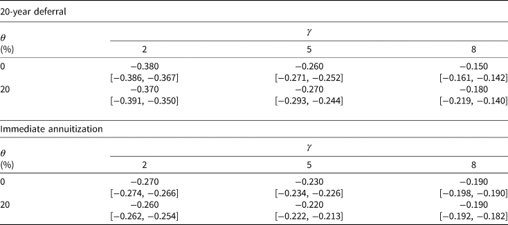
As the accuracy of longevity forecast depends on its horizon, the preference for either contract may be sensitive to the age when the individual annuitizes. In the baseline case, individuals are aged 25 when purchasing a DVA contract or participating in the GSA. As retirement benefit payments commence at age 66, the deferral period is 40 years. When the deferral period is shorter, survival probability forecasts are more accurate. Thus, we expect smaller differences in the average level and standard deviation of benefits between contracts. However, this does not necessarily imply that the CEL estimates would be closer to zero, because the time-preference discounting, as governed by the subjective discount factor, β in equation (2), plays a larger role when retirement is imminent. Thus, while the difference between the benefits would be smaller, the effect in terms of utility would be greater. By shortening the deferral period to 20 years, we find that the effect due to shorter time-discounting dominates the more accurate probability forecast, while for immediate annuitization, the effects are mixed. In all cases, the CEL estimates are negative and statistically significant across all γs (Table 5).
Table 5. Deferral period: CEL (%). The top panel displays the CEL, equation (11), for individuals aged 45 at annuitization, whereas the bottom panel corresponds to the CELs for individuals aged 65 at that time. All other parameters are identical to those in the baseline case. The 99% confidence intervals estimated by the Delta method are in parentheses
6.1.2 Stock exposure
As long as the allocation to the stock index corresponds to an optimal AIR with similar default rates as those in the baseline case, individuals prefer the GSA.
We consider four alternative exposures to the stock index. The first three are constant allocations over the planning horizon:  $\theta _1 = 40\%, \;\theta _2 = 60\%, \;\theta _3 = \lambda _S/\gamma \sigma _S$. θ 3 corresponds to the individual's optimal exposure to stocks (see Appendix A). For the least risk-averse individual (γ = 2), θ 3 is 147.2%. The moderately risk-averse individual (γ = 5) optimally invests 58.9% in the stock index whereas the most risk-averse individual (γ = 8) optimally invests 36.8% in stocks. The fourth exposure that we consider is an age-dependent allocation that begins with around 90% allocation to stocks at age 25, and gradually diminishes to a minimum of about 30% post-retirement until the maximum age,
  $\theta _4 = \lcub {\theta_{4,\\x}} \rcub _{x = 25}^{95} $.Footnote 27
For all θs, the optimal AIRs that are set according to equation (5) are higher than those in the baseline case. Due to the inverse relationship between the default rate and the AIR, the default rates are marginally smaller than those in the baseline case. Consequently, individuals prefer the GSA to a similar extent as in the baseline case.
6.2 Features that directly affect default rates
We investigate an individual's preference between the DSA and the GSA at various default rates. The DVA provider's CDRs are directly affected by systematic longevity risk when equity capital is kept constant, or alternately, the level of equity capital when systematic longevity risk is held constant. When higher DVA provider default rates manifest via a lower level of equity capital, or a higher standard deviation of the longevity model time trend (i.e., higher σ δ), the extent to which the individual prefers the GSA is greater. As the DVA provider's default rates are only slightly affected by the standard deviation of the age-dependent errors on the mortality matrix (σ x) and parameter uncertainty of the time trend's drift term, c, these two sources of uncertainty do not influence the individual's preference for the GSA.
6.2.1 Consequential
The level of equity capital and σ δ have consequential effects on the default rates. A lower level of equity capital or a higher σ δ increases the CDR, hence individuals prefer the GSA more, as indicated by the CELs that are decreasing in CDRs (Figures 5 and 6).Footnote 28 Moreover, the extent to which individuals prefer the GSA relative to the DVA with respect to their risk aversion levels varies with the CDR, i.e., the curves intersect. At low levels of CDR, risk averse individuals have a weaker preference for the GSA relative to a more risk averse individual. This is due to the appeal of more stable benefits under a DVA from a sound provider. When there is a small amount of default risk of about 0.5%, more risk averse individuals soon find the DVA to be less attractive than the GSA. Individuals' preference for the DVA diminishes in the CDR regardless of whether the high default rates are induced by heightened systematic longevity risk or less equity capital. Additionally, individuals have a slight preference for the GSA over a zero-default-risk DVA, as seen from a negative CEL when CDR is zero. This is due to the asymmetric effect that longevity time-trend shocks in the Lee and Carter (Reference Lee and Carter1992) model have on the benefit adjustments. A negative shock which causes life expectancy decline results in larger upward benefit adjustment than the downward benefit adjustment that a positive shock of the same magnitude entails.

Figure 5. CEL and CDR: varying level of equity capital. This figure presents the CEL and CDR for the base case's risk aversion levels, γ. The CDR is altered by changing the level of equity capital from 0% to 12.5% of the contract's best estimate value. The top panel is for  $\theta = 0\% $, whereas the bottom panel is for
  $\theta = 20\% $. The data points are based on simulations with 100,000 replications.

Figure 6. CEL and CDR: varying σ δ. This figure presents the CEL and CDR for the base case's risk aversion levels, γ. The CDR is altered by changing σ δ from 0 to 2 times the calibrated value in the base case. The top panel is for  $\theta = 0\% $, whereas the bottom panel is for
  $\theta = 20\% $. The data points are based on simulations with 100,000 replications.
6.2.2 Inconsequential
The standard deviation of errors on the mortality matrix (σ x) and drift parameter uncertainty affect the default rates only marginally. Hence, the baseline results are unchanged.
The time trend in the Lee and Carter (Reference Lee and Carter1992) model accounts for the bulk of the uncertainty surrounding systematic longevity evolution. Thus, even when σ x is five times as large as the calibrated values, CDRs and CELs deviate little from those in the baseline case.
When there is uncertainty around the drift parameter, the DVA is disadvantaged by a higher default probability. However, the GSA's appeal also diminishes as entitlement adjustments have a wider variation, especially near the maximum age. Neither of these drawbacks is sufficiently decisive to sway individual preferences. Therefore, the CELs differ only marginally from those in the baseline case. The incorporation of parameter uncertainty is described in Appendix D.
6.3 Alternate longevity model
We next explore the choice of the longevity model by replacing the Lee and Carter (Reference Lee and Carter1992) model with the Cairns et al. (Reference Cairns, Blake and Dowd2006) model, which produces a wider range of survival probabilities at old age. We calibrate the Cairns et al. (Reference Cairns, Blake and Dowd2006) model over the same sample of mortality data as that in Section 3.2. Figure 7 presents the fan plot of the simulated fraction of living individuals under the Cairns et al. (Reference Cairns, Blake and Dowd2006) model. The maximum range of the fraction of 25-year-olds still alive at older ages is 45% (i.e., at age 91), 50% more than the maximum range under the Lee and Carter (Reference Lee and Carter1992) model (i.e., 30% interval at age 88; Figure 2). This wider range translates into greater variability in benefits for the GSA, and higher default rates for the DVA provider.
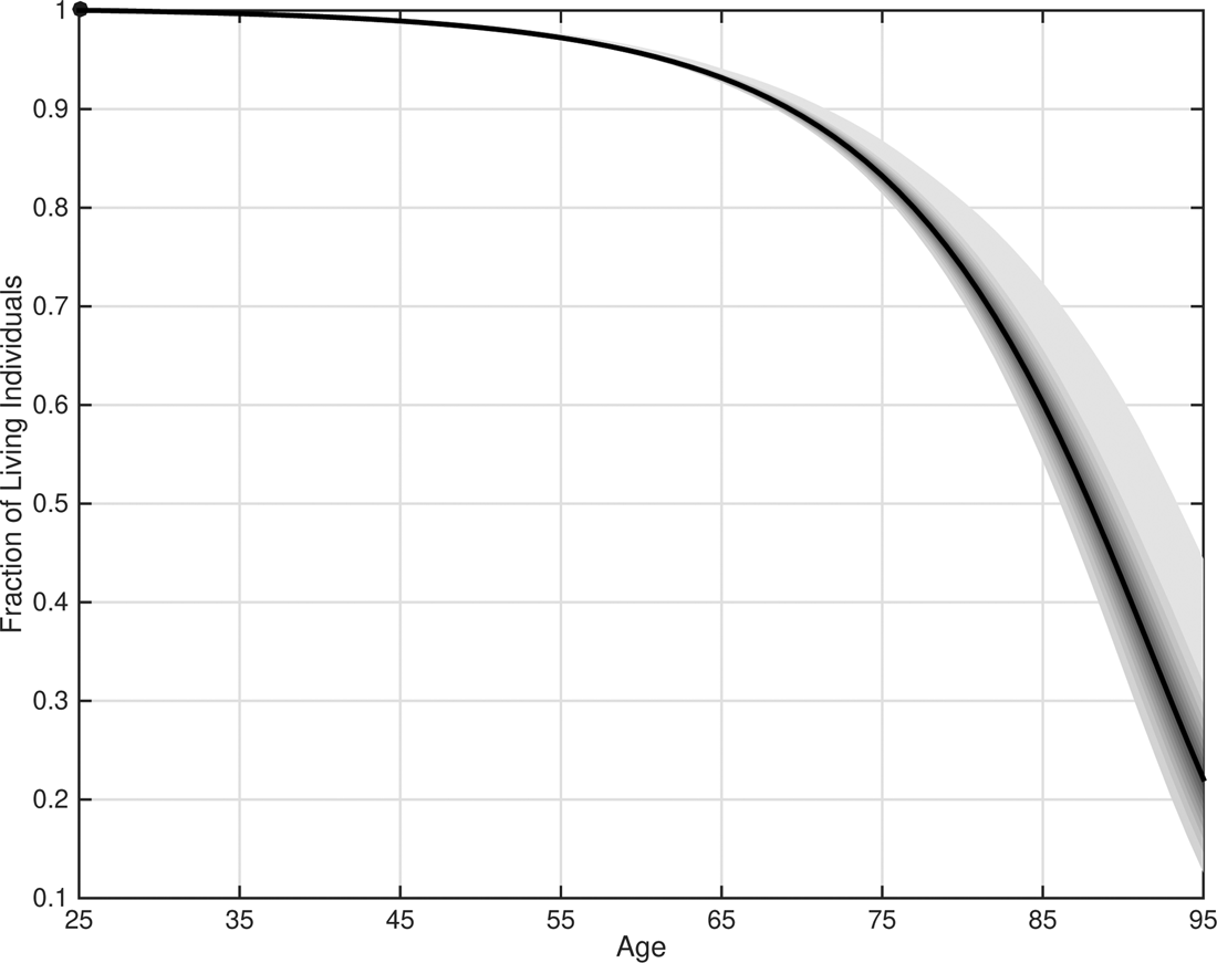
Figure 7. Mortality model: fan plot. This figure presents the fan plot of the simulated fraction of living individuals (i.e., the population of 25-year-olds is normalized to one) over 10,000 replications when longevity is modeled according to the Cairns et al. (Reference Cairns, Blake and Dowd2006) model. The model is calibrated on US female death counts from 1980 to 2013 taken from the Human Mortality Database. Darker areas indicate higher probability mass.
With either the Lee and Carter (Reference Lee and Carter1992) or the Cairns et al. (Reference Cairns, Blake and Dowd2006) model, the rise in GSA benefits with age is accompanied by more uncertainty surrounding the benefits. However, the Cairns et al. (Reference Cairns, Blake and Dowd2006) model produces greater uncertainty as the individual ages, as seen by comparing the top panels in Figures 3 and 8. This generates greater individual preference for the DVA under the Cairns et al. (Reference Cairns, Blake and Dowd2006) model.

Figure 8. Mortality model: box plots of GSA and DVA benefits. This figure presents the box plots of benefits for the GSA (top panel) and the DVA (bottom panel), for an individual with a risk aversion level of γ = 5, at ages 66, 80, and 95. The underlying portfolio is invested in the money market account only. The line in the middle of the box is the median, while the edges of the box represent the 25th and 75th percentiles. The height of the box is the interquartile range, i.e., the interval between the 25th and 75th percentiles. The ‘+’ symbols represent data points 1.5 times larger than the interquartile range.
For a fixed level of equity capital, the Cairns et al. (Reference Cairns, Blake and Dowd2006) model yields higher default rates because of the heightened uncertainty surrounding old age survival. If we maintain the baseline case's 90% leverage ratio, the default rates under the Cairns et al. (Reference Cairns, Blake and Dowd2006) model are between 0.48% and 2.21% (Table 6), substantially higher than the at-most 0.01% default rates when the Lee and Carter (Reference Lee and Carter1992) model is adopted (Table 2). Consequent to more defaults, individuals have a lower preference for the DVA (Table 6, bottom panel), as the CEL estimates are more negative than those in the baseline case (Table 3). Therefore, individuals prefer the DVA contract under the Cairns et al. (Reference Cairns, Blake and Dowd2006) model only if the associated default risk is curtailed. Despite that, regardless of whether equityholders provide enough capital to eliminate default risk, the Sharpe ratio of equity provision is lower than the ratio of abstaining from systematic longevity risk exposure. The Jensen's α of equity provision is positive but economically insignificant.
Table 6. Mortality model with default: CDRs (%) and CEL (%). The top panel presents the CDRs, equation (9), whereas the bottom panel displays the CEL, equation (11), when life expectancy follows the Cairns et al. (Reference Cairns, Blake and Dowd2006) model, calibrated to the same sample as the Lee and Carter (Reference Lee and Carter1992) model. All other parameters are identical to those in the baseline case. The 99% confidence intervals are in parentheses

Additionally, the choice of the longevity model underlies the inference of Maurer et al. (Reference Maurer, Mitchell, Rogalla and Kartashov2013). While we find that individuals marginally prefer the GSA, Maurer et al. (Reference Maurer, Mitchell, Rogalla and Kartashov2013) observe the opposite (positive CEL for the contract indexed to systematic longevity; Table 7 of Maurer et al., Reference Maurer, Mitchell, Rogalla and Kartashov2013). When we assume that no default occurs, as do Maurer et al. (Reference Maurer, Mitchell, Rogalla and Kartashov2013), we are able to reconcile our results to theirs. For instance, individuals who are moderately risk-averse to risk-averse, γ = 5 and 8, prefer the DVA; Table 7, top panel. The most risk-averse individual is willing to pay as much as 1% in loading to shed systematic longevity risk. Despite that, when the annuity provider sets the loading to be equal to the CEL, the accompanying Sharpe ratio remains inferior to the Sharpe ratio of investing in only the financial market, i.e., 0.45 when  $\theta = 20\% $, whereas the Jensen's α is positive but economically insignificant (Table 7, bottom panel). Therefore, while individual preference is sensitive to the choice of the longevity model, the extent that individuals are willing to pay to insure against systematic longevity risk is insufficient to entice equityholders to gain exposure to that risk.
Table 7. Mortality Model with No Default: CEL (%) and Investment Performance Statistics. The top panel presents the CEL, equation (11), when life expectancy follows the Cairns et al. (Reference Cairns, Blake and Dowd2006) model, calibrated to the same sample as the Lee and Carter (Reference Lee and Carter1992) model. The bottom panel shows the Sharpe ratio (SR) and Jensen's α, equation (12), when the loading is set at the CEL estimates in the top panel. Equity capital is sufficiently high such that no default occurs. All other parameters are identical to those in the baseline case. The 99% confidence intervals are in parentheses

6.4 Contract combination
The analysis thus far assumes that the individual can select either the DVA or the GSA but not both. In Figure 9, we show the optimal weight allocated to a DVA contract with no loading for various CDRs when there is no investment in stocks (θ = 0). When the DVA provider has no default risk, the most risk-averse individual, γ = 8, optimally holds around 44.8% of the annuitization wealth in the DVA. The optimal holding for a less risk-averse individual, γ = 5, is markedly smaller at 11.8%. The least risk-averse individual, γ = 2, never finds it optimal to purchase a DVA contract regardless of the provider's default risk. Risk-averse individuals find it more appealing to purchase a DVA with low or zero default risk because the DVA offers a less volatile benefits.

Figure 9. Optimal allocation to DVA, CEL, and CDR:  $\theta = 0\% $. The top panel displays the optimal allocation, ω*, to the DVA, for an annuitization wealth that is normalized to 1 (1 − ω* is thus used to purchase the GSA), for various levels of CDR and
  $\theta = 0\% $. The bottom panel shows the CEL for the DVA in the optimal contract combination, for various levels of CDR. The CDR is altered by changing the level of equity capital from 0% to 12.5% of the contract's best estimate value.
However, the increase in expected utility from contract combination is small, as measured by the level of loading on the DVA (CEL) that equates the individual's expected utility under the GSA and the optimal DVA/GSA mix. This CEL is less than 0.18% for the most risk-averse individual for the DVA contract with no default risk. This positive but low CEL generates insufficient reward to entice equityholders to provide capital to the DVA provider. Instead, equityholders are better off investing in the stock market only. When contracts are 20% invested in the stock index, we obtain comparable optimal DVA contracts purchased, CEL, and inference on the equityholders' investment performance. For instance, for γ = 8,  $\theta = 20\% $ and equity capital of 12.5%, offering the DVA with a loading equivalent to the CEL of 1.6 b.p. realizes a Sharpe ratio of 0.34 for equityholders, which is less than the Sharpe ratio of 0.45 of investment in the financial market only.Footnote 29 Thus, the DVA provider is unable to adequately compensate equityholders when individuals can allocate between the two contracts.
Allowing the individual to allocate annuitized wealth between the two options is appealing to individuals who are at least moderately risk-averse (γ ≥ 5), and only when the DVA provider's default risk is small. Even though a combination of contracts is welfare-enhancing, the expected utility improvement is so small that equityholders are not sufficiently compensated for bearing systematic longevity risk.
7. Conclusion
We investigate systematic longevity risk management in retirement planning in the presence of two alternatives: individuals participate in a collective scheme that adjusts retirement income according to longevity evolution, or purchase a variable annuity contract offered by an equityholder-backed annuity provider. Our model features the perspective of not only the individuals, who evaluate their welfare in retirement, but also of the equityholders, who weigh their risk-return tradeoff from systematic longevity risk exposure.
Due to the entitlement adjustments arising from errors in survival probability forecasts, the collective scheme provides more volatile benefits than those of an annuity contract. However, the collective scheme also offers a slightly higher average level of benefits, because for errors of the same magnitude, over- and under-estimating the log central death rates produce asymmetric effects.
The annuity contract provider relies on limited equity capital to subsume forecasting errors, and so is subject to default risk. Although the annuity contract shields individuals from downward entitlement adjustments up to a limit, it deprives individuals of any upward adjustments, as these gains belong to the equityholders.
We find that individuals marginally prefer the collective scheme over the annuity contract priced at its best estimate. This implies that the annuity provider is unable to charge a positive loading on the contract, subsequently failing to compensate its equityholders who bear longevity risk. Therefore, when individuals have the choice to form a collective scheme, the annuity provider who has no advantage at managing systematic longevity risk, and who has to fully hedge financial market risk would not exist in equilibrium. Our finding is robust to individuals' risk aversion level, the contract deferral period, and stock market risk exposure. Individuals' desire for an annuity contract diminishes in the provider's default risk regardless of whether the underlying determinant of default risk is the magnitude of systematic longevity risk or the level of equity capital. When faced with higher systematic longevity risk, individuals are willing to purchase an annuity contract with no default risk, but the loading that individuals offer remains insufficient to compensate the equityholders for taking systematic longevity risk. Individuals can attain higher expected utility by optimally allocating their wealth at retirement between the two contracts. In this instance, the risk-averse individuals are willing to offer a positive loading, but the loading is also insufficient as a reward to the equityholders.
The results advocate for collective mechanisms in pension provision, which exist in a handful of countries (e.g., Collective Defined Contribution in the Netherlands, Target Benefit Plans in Canada). The pressing issue of population aging, and the gradual maturation of the longevity risk derivatives market, is likely to spur reform. For example, the US Chamber of Commerce (2016) recommends new plan designs to enhance the private retirement system. Our results also highlight the difficulty for insurers to offer long-term guarantees on non-diversifiable risks such as systematic longevity, while offering an attractive remuneration to their shareholders.
A limitation of our work is the exclusion of channels that may reduce the insurer's effective longevity exposure, such as synergies in product offering (e.g., natural hedging of systematic longevity risk via the sale of annuities and life insurance contracts; Gatzert and Wesker, Reference Gatzert and Wesker2012; Wong et al., Reference Wong, Sherris and Stevens2017), access to reinsurance (Baione et al., Reference Baione, De Angelis, Menzietti and Tripodi2017), and shadow insurance (Koijen and Yogo, Reference Koijen and Yogo2016). In such a scenario, the annuity contract could be sold at a lower price. In the base case scenario, our results suggest that individuals would choose the DVA only when it is priced lower than the actuarial best estimate price. There are also alternative resolutions in the case of default, and other factors that may influence annuitization decisions, such as bequest motives, medical expenses, social security, uninsurable income, etc. (Lockwood, Reference Lockwood2012; Pashchenko, Reference Pashchenko2013; Yogo, Reference Yogo2016; Ai et al., Reference Ai, Brockett, Golden and Zhu2017; Peijnenburg et al., Reference Peijnenburg, Nijman and Werker2017). Additionally, when the number of individuals is not large enough to assume away idiosyncratic longevity risk, it may become a larger risk driver of benefits relative to the systematic component of longevity risk. Examining these features in future research would enrich our knowledge of retirement planning.
Acknowledgement
We gratefully acknowledge research funding from Observatoire de l'Epargne Européenne. We thank the editor, O. Mitchell, two anonymous referees, D. Blake, D. Davydoff, A.M.B. De Waegenaere, N. Gatzert, J. Glachant, C. Gollier, P. Lopes, E. Luciano, A. Michaelides, G. Nicodano, T.E. Nijman, E. Vigna, R. Zhou, as well as the participants of the Longevity 12 Conference, Netspar International Pension Workshop 2017, American Risk and Insurance Association (ARIA) 2017 Annual Meeting, and ‘Household Finance and Retirement Savings’ Workshop of the Center for Research on Pensions and Welfare Policies (CeRP). The views and opinions expressed here do not necessarily reflect that of Aegon and/or its clients.
Appendix A
Rationale of the contract definition
The DVA and GSA contracts are not only modeled along the variable annuity contracts studied in the literature (Koijen et al., Reference Koijen, Nijman and Werker2011; Maurer et al., Reference Maurer, Mitchell, Rogalla and Kartashov2013), but are also relatable to an individual's optimal consumption and investment.
The problem of optimal consumption and investment is composed of two separate parts: the allocation of initial wealth over each retirement year, and the investment strategy. Aase (Reference Aase2015) shows that for an expected-CRRA-utility-maximizing individual facing idiosyncratic longevity and stock market risks, the optimal allocation of initial wealth decays geometrically in the retirement horizon. The AIR in our setting represents precisely this rate of decay.
When individuals are subject to longevity risk, its existence would not change the optimal wealth and asset allocation; complication to the solution arises from the inability to react to longevity evolution (Huang et al., Reference Huang, Milevsky and Salisbury2012). We, however, assume that the contract's parameters are deterministic (i.e., fixed in the year when it is sold, and the incorporation of new information thereafter is prohibited). Therefore, by an appropriate choice of the AIR, h*, the contract described by equations (3) and (4) coincides with the optimal decumulation path of the individual.
We next solve the utility maximization problem, (13), to obtain the optimal AIR and investment strategy for a contract defined by equations (3) and (4).
At time t 0, the individual purchases the maximum number of variable annuity contracts affordable with a lump sum capital normalized to one. The annuity contract commences benefit payment in year t R, until the year t, conditional on the individual's survival. In the financial market setting as described in Section 2.1, with a deterministic fraction of wealth  $\theta = \lcub {\theta_t} \rcub _{t = t_0}^T $ invested in the risky stock index, and 1 − θ invested in the money market account, the value of the reference portfolio evolves according to
  ${\rm d}W_t/W_t = \lpar {r + \theta_t \;\lambda \sigma_S} \rpar {\rm d}t + \theta _t\sigma _S{\rm d}Z_{S,t}$:
 $$\eqalign{\mathop {\max} \limits_{\lcub {\theta_t,h\lpar {t,\;\theta_t} \rpar } \rcub _{t = tR}^T} = & \, {\rm {\opf E}}_{t_0}[ {U\lpar \Xi \rpar } ] \cr = & \, {\rm {\opf E}}_{t_0}\left[ {\int_{t_R}^T {{\rm e}^{-\beta (t-t_0)}} \displaystyle{{\Xi_t^{1-\gamma}} \over {1-\gamma}} \left( {\prod\nolimits_{s = t_0}^t {{}_1p_{x + (s-t_0)}^{(s)}}} \right){\rm d}t} \right] \cr \Xi _t = &\left\{ {\matrix{ {\displaystyle{1 \over {A(h)}}\exp (-h(t,\theta_t)(t-t_R))\displaystyle{{W_t} \over {W_{t_0}}}} \hfill & {{\rm if}\;{\rm alive}\;{\rm in}\;{\rm year}\;t} \hfill \cr 0 \hfill & {{\rm otherwise}} \hfill \cr}} \right\} \cr A(h) = &\int_{t_R}^T {\exp (-h(t,\theta _t)(t-t_R)) \times {\rm {\opf E}}_{t_0}} \left[ {\left( {\prod\nolimits_{s = t_0}^t {{}_1p_{x + (s-t_0)}^{(s)}}} \right)} \right]{\rm d}t \cr h(t,\theta _t) = & \,{\rm AIR} \cr \beta = & \,{\rm subjective}\;{\rm discount}\;{\rm factor} \cr \gamma = & \, {\rm risk}\;{\rm aversion}\;{\rm parameter} \cr W_t = &\, {\rm value}\;{\rm of}\;{\rm the}\;{\rm reference}\;{\rm portfolio}\;{\rm with}\;{\rm the}\;{\rm investment}\;{\rm policy} \theta \cr {\rm {\opf E}}_{t_0} = \left[ {\prod\nolimits_{s = t_0}^t {{}_1p_{x + (s-t_0)}^{(s)}}} \right] = &{}_{t-t_0}p_x^{(t_0)}} $$
A(h) is the cost per unit of a zero-loading contract. It is straightforward to verify that the contract has a present expected value of one for any  $h\in {\rm {\opf R}}^{T-t_R}$, and thus satisfies the budget constraint. Given any θ, the first order condition,
  $\partial {\rm {\opf E}}_{t_0}[ {U\lpar \Xi \rpar } ] /\partial h = 0$ yields the optimal AIR, equation (14):
 $$\eqalign{h^{^\ast}\lpar {t,\;\theta_t} \rpar = & \, r + \displaystyle{{\beta -r} \over \gamma} -\displaystyle{{1-\gamma} \over \gamma} \theta _t\sigma _S\left( {\lambda_S-\displaystyle{{\gamma \theta_t\sigma_S} \over 2}} \right) \cr r = & \,{\rm constant}\;{\rm short}\;{\rm rate} \cr \beta = & \,{\rm subjective}\;{\rm discount\;} \;{\rm factor} \cr \gamma = & \, {\rm risk}\;{\rm aversion}\;{\rm parameter} \cr \theta _t = & \,{\rm fraction}\;{\rm of}\;{\rm wealth}\;{\rm allocated}\;{\rm to}\;{\rm the}\;{\rm stock}\;{\rm index}\;{\rm at}\;{\rm time}\;t,\;t_R \le t \le T \cr \sigma _S = & \,{\rm standard}\;{\rm deviation}\;{\rm governing}\;{\rm the\;} \;{\rm stock}\;{\rm index^{\prime}s}\;{\rm dynamics} \cr \lambda _S = & \,{\rm instantaneous}\;{\rm Sharpe}\;{\rm ratio}\;{\rm of}\;{\rm the}\;{\rm stock}\;{\rm index}} $$
Equation (14) is composed of the risk-free rate, the difference between the subjective discount factor and the risk-free rate, adjusted by the risk aversion parameter, and a term concerning the exposure to the stock index, weighted by the risk aversion level.
If the returns on the investment were constant at r (e.g., either θ = 0 or σ S = 0), for any given level of risk aversion, γ, the shape of the optimal consumption path depends on the relative magnitude of β and r. An individual who discounts future consumption at a higher rate than the constant interest rate (i.e., β > r, an impatient individual) prefers a downward sloping consumption path whereas a more patient person (i.e., β < r) optimally chooses an upward sloping path. When θ ≠ 0 and σ S ≠ 0, then the risk aversion level, the standard deviation and the market price of stocks also have a role in determining the optimal consumption path.
The first-order condition corresponding to the allocation to the stock index,  $\partial E_{t_0}[ {U\lpar \Xi \rpar } ] /\partial \theta = 0$, implies the optimal allocation to the risky asset:
 $$\theta^{\ast} = \displaystyle{{\lambda _S} \over {\gamma \sigma _S}}$$
The optimal allocation to the stock index, θ*, is independent of time and wealth, and is identical to the optimal investment policy of Merton (Reference Merton1969).
The variable annuity contract provides the optimal decumulation path when the AIR is set to  $h^*\lpar {t,\theta_t^*} \rpar $. By prohibiting the incorporation of new information into the contract definition after its date of sale (i.e., enforcing deterministic, but possibly time-varying contract parameters), longevity risk does not influence the optimal AIR and the optimal portfolio choice.
The conception of the GSA as a collective justifies the assumption that it prioritizes individual welfare (i.e., maximizes individuals' expected utility in retirement). Therefore, the GSA offers an AIR that is in the best interest of the individuals, without conflict among its stakeholders. As for the annuity provider, such contracts are also conceivable. For instance, Froot (Reference Froot2007) suggests that insurers should shed all liquid risks for which they have no comparative advantage to outperform (e.g., financial market risk), and devote their entire risk budget to insurance risks (e.g., longevity risk). The selling of variable annuities without any financial guarantee achieves precisely this goal. Besides, Gatzert et al. (Reference Gatzert, Holzmüller and Schmeiser2012) demonstrate that if an insurance company sets contract parameters for a participating life insurance contract such that they maximize the contract's value (e.g., expected utility) to the individual, the individual may be willing to pay more for the contract. Therefore, the provision of contracts defined according to equations (3) and (4) under either a cooperative setup or by a for-profit entity is plausible.
Appendix B
Definition of the book value of liabilities
Suppose that the DVA provider or the GSA administrator issues contract(s) to a cohort who is aged x at time t 0, promising entitlements of  $\Xi ^K\lpar {h^*,\;F,\;t,\;x} \rpar, \;K\in \lcub {DVA,\;GSA} \rcub $, in every year t, t R ≤ t ≤ T, conditional on the individual's survival. The estimate of the entity's book value of liabilities at time t, t 0 ≤ t ≤ T, is:
 $$\eqalign{L_t\equiv &\Xi ^K\lpar {h^{^\ast},F,t,x} \rpar \int_{s = \max \lcub {t_R,t} \rcub }^T {\exp \lpar {-h^{^\ast}\lpar {s,\theta} \rpar \lpar {s-t} \rpar } \rpar \times _{s-t}^{} p_{x + t-t_0}^{\lpar t \rpar } {\rm ds}} \cr {}_{s-t}p_{x + t-t_0}^{(t)} = & \, {\rm conditional}\;{\rm probability}\;{\rm in}\;{\rm year}\;t\;{\rm that}\;{\rm a}\;{\rm living}\;{\rm individual} \cr & \quad {\rm of}\;{\rm age}\;x{\rm}+{\rm } t\;{\rm lives}\;{\rm for}\;{\rm at}\;{\rm least}\;s-t\;{\rm more}\;{\rm years} \cr h^{^\ast}{\rm (}t{\rm,} \theta {\rm )} = & \,{\rm optimal}\;{\rm AIR,}\;{\rm Equation}\;{\rm (14)} \cr \Xi ^K{\rm (}h^{^\ast}{\rm,} \,F{\rm,} \,t{\rm,} \,x{\rm )} = & \,{\rm benefit}\;{\rm at}\;{\rm time}\;t\;{\rm for}\;{\rm contract}\;K\in {\rm \{} GSA{\rm,} \,DVA{\rm \}}} $$
B.1 Illustration of the case with no risk
To motivate the definition of equation (16), let us consider a three-period case (t = t 0, t 1, t 2) in the absence of stock market and longevity risks. Assume that the individual buys exactly one unit of the retirement contract at retirement in year t 0, lives with certainty to collect the benefits in year t 1 = t 0 + 1, and dies with certainty before the year t 2 = t 1 + 1. Suppose that the reference portfolio is fully invested in the money market account, earning an interest rate that is constant at 2%. Furthermore, we adopt a constant AIR,  $h = 3\% $, and zero contract loading, F = 0. As there is no uncertainty in this example, equation (16) should yield precisely the value of liabilities at time t.
By definition of the DVA contract, there are two payments to be made: one in the year t 0 and another in the year t 1. The individual receives a payment immediately, in t 0, that is valued at:
 $$\eqalign{\Xi \lpar {h,\;0,\;t_0,\;x} \rpar = & \,1 \times \displaystyle{{W_{t_0}^{Ref}} \over {W_{t_0}^{Ref}}} {\rm e}^{-h \times \lpar {t_0-t_0} \rpar } \cr = & \, 1} $$
The second payment, in present value at time t 1 is:
 $$\eqalign{\Xi \lpar {h,\;0,\;t_1,\;x} \rpar = & \,1 \times \displaystyle{{W_{t_1}^{Ref}} \over {W_{t_0}^{Ref}}} {\rm e}^{-h \times \lpar {t_1-t_0} \rpar } \cr = &\,\displaystyle{{W_{t_0}^{Ref} {\rm e}^{0.02}} \over {W_{t_0}^{Ref}}} {\rm e}^{-h} \cr = & \,{\rm e}^{-h + 0.02} \cr = & \,{\rm e}^{-0.01}} $$
Discounting equation (17) by the constant interest rate, we obtain the present value at time t 0, of the payment due at time t 1:
 $$\eqalign{PV_{t_0}[ {\Xi \lpar {h,\;0,\;t_1,\;x} \rpar } ] = & \,\Xi \lpar {h,\;0,\;t_1,\;x} \rpar {\rm e}^{-0.02 \times \lpar {t_1-t_0} \rpar } \cr = & \, {\rm e}^{-0.01-0.02} \cr = & \,{\rm e}^{-0.03}} $$
The present value of liabilities at time t 0 is
 $$\Xi \lpar {h,\;0,\;t_0,\;x} \rpar + PV_{t_0}[ {\Xi \lpar {h,\;0,\;t_1,\;x} \rpar } ] = 1 + {\rm e}^{-0.03}$$
It remains to show that equation (16) yields equation (18):
 $$\eqalign{L_t = & \, \Xi \lpar {h,\;0,\;t_1,\;x} \rpar \times \lpar {\rm e}^{-h \times 0}_0 p_t^{\lpar t \rpar} + {\rm e}^{-h \times 1}_1 p_t^{\lpar t \rpar} \rpar \cr = & \, 1 \times \lpar {1 + {\rm e}^{-h}} \rpar \cr = &\, 1 + {\rm e}^{-0.03}} $$
B.2 Illustration of the general case
We price the liabilities of the pension provision entity by constructing a replicating portfolio for its contractual obligation. We demonstrate that the price of the portfolio that replicates all the cash flows of an annuity contract is equation (16).
In the setting with systematic but no idiosyncratic longevity risk, we consider the liability associated with a contract holder who purchased 1/A unit(s) of contracts when aged x in the year t 0 = 0, retired in the year t = t R, while being subject to unknown survival probabilities throughout the horizon, until the maximum age in the year t = T, when death is certain.
The pension provision entity is contractually obliged to make annual benefit payments from the individual's retirement in the year t = t R until he or she attains maximum age in the year t = T, conditional on her survival. Let  $W_t^{Ref} $ be the price at time t of the reference portfolio to which the benefits are indexed, t ∈ [t 0, T].
Absent longevity risk, by purchasing the sum of all the units of the reference portfolio in column (2) of Table 8 at time t, the annuity provider would be able to fulfill its contractual obligation with certainty. For instance, to meet the payment at time t R, the annuity provider purchases  $1{\rm /}\lpar {AW_{t_0}^{Ref}} \rpar {\rm e}^{-h \times 0}_{t_R-t} p_x^{\lpar {t_0} \rpar } $ units of the reference portfolio at time t 0. When longevity risk is absent, the conditional expectation, made at time t 0, of the individual's survival in year t R coincides with the realized survival probability, i.e.,
  $_{t_R-t}^{} p_x^{\lpar {t_0} \rpar } = _{t_R-t}^{} p_x$. The value of this portfolio will evolve along with the financial market, to be worth exactly
  ${1 \over A}{{W_{t_R}^{Ref}} \over {W_{t_0}^{Ref}}} \times \prod\nolimits_{l = t_0}^{t_R-1} {_{l-t_0}^{} p_{x + l-t_0}^{\lpar l \rpar }} $, the payment due at time t R. By the same reasoning for the rest of the entries in column (2), equation (19) is thus the total units of the reference portfolio to be held at any time t, such that the pension provision entity fully hedges financial market risk:
 $$\int_{s = \max \lcub {t_R,t} \rcub }^T {\displaystyle{1 \over A}\displaystyle{1 \over {W_{t_0}^{Ref}}} {\rm e}^{-h\lpar {s-t_R} \rpar }_{s-t} p_{x + t-t_0}^{\lpar t \rpar } \;{\rm d}s} $$
Equation (19) is an estimate of the liabilities at time t, in terms of the units of reference portfolio. Each unit is worth  $W_t^{Ref} $ at time t. To obtain the value of liabilities, we take the portfolio's corresponding value:
 $$W_t^{Ref} \times \int_{s = \max \lcub {t_R,t} \rcub }^T {\displaystyle{1 \over A}\displaystyle{1 \over {W_{t_0}^{Ref}}} {\rm e}^{-h\lpar {s-t_R} \rpar }_{s-t} p_{x + t-t_0}^{\lpar t \rpar } \;{\rm ds}} $$
As  $\Xi \lpar {h,\;F,\;t,\;x} \rpar = W_t^{Ref} {\rm /}{\rm \bond} \lpar {AW_{t_0}^{Ref}} \rpar {\rm e}^{-h\lpar {t-t_R} \rpar }$ by definition, we can substitute it into equation (20) to get
 $$L_t: = \Xi \lpar {h^{^\ast},\;F,\;t,\;x} \rpar \int_{s = \max \lcub {t_R,t} \rcub }^T {\exp \lpar {-h^{^\ast}\lpar {s,\;\theta} \rpar \lpar {s-t} \rpar } \rpar \times _{s-t}^{} p_{x + t-t_0}^{\lpar t \rpar } {\rm ds}} $$
Equation (21) is identical to equation (16).
Table 8. Future cash flow and the best replicating portfolio of the pension provision entity. This table shows the value of entitlements due in each year of retirement until maximum age (column (1)), and the corresponding best replicating portfolio in units of the reference portfolio (column (2)). The best replicating portfolio is the conditional expectation of the benefits in future value

When there is systematic longevity risk, the best replicating portfolio is identical to column (2) of Table 8, but this best estimate may not necessarily provide the exact cash flow to meet the annuity provider's contractual obligations because the realized survival probability may deviate from its conditional expectation made at time t, which then triggers the provider's default.
Appendix C
Delta method
We apply the Delta method (Theorem 5.5.4 of Casella and Berger, Reference Casella and Berger2002) to estimate the variance of the CELs, which is used to compute their confidence intervals.
Consider the function g(x, y) = (x/y)1/(γ−1) − 1. By the definition of equation (11),  $CEL = g\lpar {U\lpar {\Xi^{GSA}} \rpar, \;U\lpar {\Xi^{DVA}} \rpar } \rpar $. We estimate the CEL by plugging the expected utility into g(.),
  $g\lpar {{\rm {\opf E}}_0[ {U\lpar {\Xi^{GSA}} \rpar } ], \;{\rm {\opf E}}_0[ {U\lpar {\Xi^{DVA}} \rpar } ] } \rpar $. Theorem 5.5.24 of Casella and Berger (Reference Casella and Berger2002) suggests the following estimate for its variance:
 $$\eqalign{& {\rm Var}\lcub {g\lpar {{\rm {\opf E}}_0[ {U\lpar {\Xi^{GSA}} \rpar } ],} { {{\rm {\opf E}}_0[ {U\lpar {\Xi^{DVA}} \rpar } ] } \rpar } \rcub } \cr & \quad = g_x^2 {\rm Var}\lpar {U\lpar {\Xi^{GSA}} \rpar } \rpar + g_y^2 {\rm Var}\lpar {U\lpar {\Xi^{DVA}} \rpar } \rpar + 2g_xg_y{\rm cov}\lpar {U\lpar {\Xi^{GSA}} \rpar, {\mkern 1mu} U\lpar {\Xi^{DVA}} \rpar } \rpar \cr & g_x = g_x\lpar {{\rm {\opf E}}_0[ {U\lpar {\Xi^{GSA}} \rpar } ], {\mkern 1mu} {\rm {\opf E}}_0[ {U\lpar {\Xi^{DVA}} \rpar } ] } \rpar \cr & g_y = g_y\lpar {{\rm {\opf E}}_0[ {U\lpar {\Xi^{GSA}} \rpar } ], {\mkern 1mu} {\rm {\opf E}}_0[ {U\lpar {\Xi^{DVA}} \rpar } ] } \rpar } $$
g x and g y denote the first partial derivative of g(.) with respect to x and to y respectively.  ${\rm Var}\lpar {U\lpar {\Xi^K} \rpar } \rpar $ for K ∈ {GSA, DVA} and
  ${\mathop{\rm cov}} \lpar {U\lpar {\Xi^{GSA}} \rpar, \;U\lpar {\Xi^{DVA}} \rpar } \rpar $ are estimated by the sample variance and sample covariance.
Appendix D
Uncertainty of the drift parameter
The maximum likelihood estimate for the drift term of the longevity model is normally distributed,  $\hat{c}\~{\rm {\cal N}}\lpar {c,\;\sigma_c^2} \rpar $. Based on the sample used for the model calibration, we obtain
  $\hat{c} = -1.0689$ and
  $\widehat{{\sigma _c}} = {\rm 0}{\rm. 0521}$. Without parameter uncertainty, the best m-year-ahead forecast at time t is
  $\widehat{{k_{t + m}}} = m\hat{c} + k_t$. To incorporate parameter uncertainty, we draw c l from the distribution
  ${\rm {\cal N}}\lpar {\hat{c},\;\widehat{{\sigma_c^2}}} \rpar $ for the lth simulation replication. The time trend governing longevity is thus
  $k_{t + m,l} = mc_l + k_{t,l} + \mathop \sum \nolimits_{i = 1}^m \varepsilon_{\delta, l},\;\varepsilon _{\delta, l}\sim{\cal N}\lpar {0,\;\widehat{{\sigma_\delta^2}}} \rpar $, while the best m-year-ahead forecast relies on
  $\hat{c}$ as c l is unobserved, i.e.,
  $\widehat{{k_{t + m,l}}} = m\hat{c} + k_{t,l}$.
Appendix E
σ δ Generating zero default
When σ δ is very small, the baseline 10% equity capital ensures that the probability of default is zero. The CEL for γ = 5, 8 increases in the multiple of σ δ, conditional on zero default probability. When systematic longevity risk is small, risk averse individuals find the welfare improvement due to upward adjustments of GSA benefits outweigh the welfare cost of the scheme's more volatile payments, but this effect reverses when systematic longevity risk rises (Figure 10).

Figure 10. CEL and multiple of σ δ: CDR = 0. This figure presents the CEL and the multiple of σ δ for the base case's risk aversion levels, γ. The top panel is for  $\theta = 0\% $, whereas the bottom panel is for
  $\theta = 20\% $.


