Vector Solution for the Intersection of Two Circles of Equal Altitude

Andrés Ruiz González

doi:10.1017/S0373463307004602

Vector Solution for the Intersection of Two Circles of Equal Altitude

Published online by Cambridge University Press: 25 March 2008

Andrés Ruiz González

Show author details

Andrés Ruiz González*: Affiliation:
(Navigational Algorithms. San Sebastián.)
*: (Email: aruiz4@euskalnet.net)

Article contents

Abstract
INTRODUCTION
VECTOR EQUATION FOR THE INTERSECTION OF TWO SIMULTANEOUS CIRCLES OF POSITION
CONCLUSION
References

Rights & Permissions

Abstract

A direct method for obtaining the two possible positions derived from two sights using vector analysis instead of spherical trigonometry is presented. The geometry of the circle of equal altitude and of the two body fixes is analyzed, and the vector equation for simultaneous sights is constructed. The running fix problem is also treated.

Keywords

Circle of Equal Altitude Celestial Navigation Sight Reduction Vector Analysis

Type: Research Article
Information: The Journal of Navigation , Volume 61 , Issue 2 , April 2008 , pp. 355 - 365

DOI: https://doi.org/10.1017/S0373463307004602 [Opens in a new window]
Copyright: Copyright © The Royal Institute of Navigation 2008

1. INTRODUCTION

Most of the known methods to solve the two body problem, [Reference Gery10], [Reference Kotlaric13–Reference A'Hearn and Rossano17], [Reference Kotlaric19], [Reference Wight24–Reference Dozier Charles26], use the navigational triangle [Reference Bowditch1] and spherical trigonometry. Recursive methods using linear approximations as in [Reference Flynn18], or physics analogies [Reference Torben12] are smart approaches. Sight reduction general procedures [2–Reference Severance5], can be used to obtain the fix, but for two sights the estimated position is needed. In reference [Reference Van Allen11] an analytical solution using plane geometry is used for both solutions.

On the other hand, vector calculus is a powerful tool widely used for engineering and physics, [Reference Max9]. In navigation it is used in naval kinematics, for current calculations, (set & drift) and the great circle sailing can be formulated using the vector analysis, [Reference Earle, Michael20–Reference Wei-Kuo and Hsuan-Shih23]; in [Reference Little, Joseph27] a vector approach of celestial navigation is made. In this paper a solution for the two body problem in celestial navigation using this technique is presented. The following sub paragraphs present some concepts about the celestial circle of position, CoP.

1.1. Variables and symbols

Let us denote the dot product by • and the cross product by Λ, and a vector by $\vec{v}$ or by v. The variables used are:

1.2. The Circle of Equal Altitude

A celestial object is far enough away from the observer that the incoming light rays are nearly parallel to each other. Thus, there is a point on the surface of Earth where the object is directly overhead at a given time; this point is called the geographical position, GP, (or of a star; substellar point). Using the spherical model of the Earth, there is a circle on her surface centred about the object's geographical position where the angle between the horizon and the celestial object, called the altitude, is constant at a given instant. This circumference forms a celestial line of position, a small circle, known as a circle of equal altitude. The great circle distance from this pole to the circle is the zenith distance of the body, Zd.

At the time of observation the observer of the celestial object must be located somewhere along that circle. The geographical position of a celestial body is calculated from an ephemeris or obtained from the Nautical Almanac, and the altitude is measured with a sextant. The observed altitude is the sextant altitude corrected for index error and dip, for refraction and if appropriate corrected for parallax and semi-diameter. This process is summarized in Figure 1.

Figure 1. Circle of Equal Altitude parameters.

Geometrically a Circle of Equal Altitude is generated by the intersection of a circular cone having its vertex in the centre of the Earth, half angle α=90°-Ho, and with the vector from O to GP as its axis, with the unit sphere. The distance from the centre of the Earth to the plane containing the CoP is sin(Ho), as shown in Figure 2.

Figure 2. Earth's normal section to the plane of the Circle of Position (CoP).

1.3. Vector equation for the Circle of Equal Altitude

In Figure 3, let OP be the observer's position at the time of sight, and GP the geographical position of the celestial body at the same instant. The dot product of the vectors defined by the centre of the Earth and these points is the cosine of the angle between them, which is the zenith distance of the observed body. Then, the vector equation of the circle of equal altitude is:

(1)

$\overrightarrow O P \hskip3 {\vskip-1\scriptstyle{\bullet}} \hskip2 \overrightarrow G P \equals cos \kern1pt \lpar 90^\circ \minus Ho\rpar$

It is possible to write the azimuth in vector form [8].

Figure 3. Circle of Equal Altitude and vectors.

1.4. Coordinate Systems

Using a right-handed orthonormal basis $\lcub \vec{i}\comma \vec{j}\comma \vec{k}\rcub$ , as in Figure 4, the Cartesian system of coordinates is defined where the origin O, is the centre of the Earth with Axes:

• Z: from O to the North Pole.
• X: from O to the Greenwich meridian, included in the Earth's equatorial plane.
• Y: defined by $\vec{j} \equals \vec{k} \wedge \vec{i}$

Since angles are used, not distances, the hypothesis that the Earth is a sphere of unit radius is valid.

Figure 4. Right-handed orthonormal basis, and coordinates.

The relationship between the equatorial coordinates (Dec, GHA), and geographical coordinates (B, L), with the spherical ones, (ϕ, θ), arises from Figure 4:

$\eqalign{ \tab {\rm r \equals 1}\quad \hskip51{\rm r \equals 1} \cr \tab {\rm Dec \equals }\rmphiv \quad \hskip35{\rm B \equals }\rmphiv \cr \tab {\rm GHA \equals 360}^\circ \,{\hbox{-}} \theta \quad \hskip4.5{\rm L \equals }\theta \cr}$

According to this formulation the unit vector in Cartesian coordinates, (x,y,z), from the centre of the Earth to the geographical position of any body is:

(2)

$\overrightarrow{{\bf GP}} \equals cos \kern1pt Dec\, cos \kern1pt GHA \cdot \vec{i} \minus cos \kern1pt Dec\, sin \kern1pt GHA \cdot \vec{j} \plus sin \kern1pt Dec \cdot \vec{k}$

And the unit vector in Cartesian coordinates from the centre of the Earth to any point on the surface of the Earth is:

(3)

$\overrightarrow{{\bf OP}} \equals cos \kern1pt B\, cos \kern1pt L \cdot \vec{i} \plus cos \kern1pt B\, sin \kern1pt L \cdot \vec{j} \plus sin \kern1pt B \cdot \vec{k}$

2. VECTOR EQUATION FOR THE INTERSECTION OF TWO SIMULTANEOUS CIRCLES OF POSITION

In the general case, two CoP intersect at two points: I₁ and I₂, (Figure 5). The coordinates of these two crossings are the solution to the problem. Using the vector notation in section 1.3 there are three unknown variables, the Cartesian coordinates of OP; so three equations are needed:

(4)

$\eqalign{\tab \overrightarrow{{\bf OP}} \hskip3 {\vskip-1\scriptstyle{\bullet}} \hskip2 \overrightarrow{{\bf GP}} _{\bf \setnum{1}} \equals sin \kern1pt Ho_{\setnum{1}} \cr \tab \overrightarrow{\bf OP} \hskip3 {\vskip-1\scriptstyle{\bullet}} \hskip2 \overrightarrow{{\bf GP}} _{\bf \setnum{2}} \equals sin \kern1pt Ho_{\setnum{2}} \cr \tab \overrightarrow{\bf OP} \hskip3 {\vskip-1\scriptstyle{\bullet}} \hskip2 \overrightarrow{\bf OP} \equals 1 \cr}$

The last equation takes account of the fact that the observer is on the surface of a unit sphere: x²+y²+z²=1. To solve the system some methods have been published [Reference Watkins and Janiczek4], [Reference Van Allen11].

Figure 5. Crossing of two CoP.

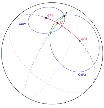
Another approach arises considering Figures 5 & 6. The great circle passing through the two geographical positions is perpendicular to the one defined by the points I₁ and I₂, and intersect in a point I_c′ on the surface of the sphere. Each CoP is contained in a plane, (section 1.2), the intersection of these planes is the line defined by the points I₁ and I₂. The line OI_c′ and the line I₁I₂ have a point in common: I_c. The vector from the centre of the Earth to each GP in rectangular coordinates is:

(5)

$\overrightarrow{{\bf GP}} _{j} \equals \lpar { {cos \kern1pt Dec_{j}\; cos \kern1pt GHA_{j} }{ \minus cos \kern1pt Dec_{j} \;sin \kern1pt GHA_{j}}\;{sin \kern1pt Dec_{j} }} \rpar$

for the two crossings j=1,2. This vector is perpendicular to the plane that contains the CoP.

Figure 6. Section by the plane containing the two geographical positions and the centre of the Earth.

The vector from the origin to the point I_c can be written like a linear combination of the GP vectors:

(6)

$\overrightarrow{{\bf OI}} _{\bf c} \equals k_{\setnum{1}} \overrightarrow{{\bf GP}} _{\bf \setnum{1}} \plus k_{\setnum{2}} \overrightarrow{{\bf GP}} _{\bf \setnum{2}}$

Where k ₁ and k ₂ are the scale factors derived from Figure 7, and alpha is the angle between the two GP vectors:

(7)

$\overrightarrow{{\bf GP}} _{\bf \setnum{1}} \hskip3 {\vskip-1\scriptstyle{\bullet}} \hskip2 \overrightarrow{{\bf GP}} _{\bf \setnum{2}} \equals cos \kern1pt \alpha$

Figure 7. Vector to the point I_c.

The direction of the line connecting the two intersection points: I₁ and I₂, is defined by the unit vector

(8)

$\vec{r} \equals {{\overrightarrow{{\bf GP}} _{\bf \setnum{1}} \wedge \overrightarrow{{\bf GP}} _{\setnum{2}} } \over {\left\Vert {\overrightarrow{{\bf GP}} _{\bf \setnum{1}} \wedge \overrightarrow{{\bf GP}} _{\setnum{2}} } \right\Vert}}$

perpendicular to the great circle passing through the two geographical positions. The vectors from I_c to the points solution of the problem are:

$\overrightarrow{{\bf I}_{\bf c} {\bf I}} _{\setnum{1}} \equals L_{\setnum{1}} \vec{r} \ {\rm and\ }\overrightarrow{{\bf I}_{\bf c} {\bf I}} _{\setnum{2}} \equals L_{\setnum{2}} \vec{r}.$

From Figure 8, L₁ and L₂ are distances from the middle point of the I₁I₂ line to each intersection point.

(9)

${\rm L}_{\rm j} {\rm \equals I}_{\rm c} {\rm I}_{\rm j} {\rm \ }$

(10)

${\rm OI}_{\rm c}^{ \hskip3\rm \setnum{2}} {\rm \plus I}_{\rm c} {\rm I}_{\rm j}^{\hskip3\rm \setnum{2}} {\rm \equals OI}_{\rm j}^{\hskip3\rm \setnum{2}} {\rm \equals 1\ }$

where j=1,2.

Figure 8. Section by the plane containing the line I₁I₂and O.

OI_c is obtained using the dot product:

(11)

$\overrightarrow{{\bf OI}} _{\bf c} \,{\vskip-2\scriptstyle{\bullet}}\, \overrightarrow{{\bf OI}} _{\bf c} \equals OI_{c}^{\setnum{2}}$

(12)

$L_{j} \equals \pm \sqrt {1 \minus \overrightarrow{{\bf OI}} _{\bf c} \,{\vskip-2\scriptstyle{\bullet}} \, \overrightarrow{{\bf OI}} _{\bf c} }$

The vector from the origin to each intersection is:

(13)

$\overrightarrow{{\bf OI}} _{j} \equals \overrightarrow{{\bf OI}} _{\bf c} \plus \overrightarrow{{\bf I}_{\bf c} {\bf I}} _{\bf j}$

And finally, the vector equation for the solution points is:

(14)

$\overrightarrow{{\bf OI}} _{j} \equals k_{\setnum{1}} \overrightarrow{{\bf GP}} _{\bf \setnum{1}} \plus k_{\setnum{2}} \overrightarrow{{\bf GP}} _{\bf \setnum{2}} \plus L_{j} {{\overrightarrow{{\bf GP}} _{\bf \setnum{1}} \wedge \overrightarrow{{\bf GP}} _{\setnum{2}} } \over {\left\Vert {\overrightarrow{{\bf GP}} _{\bf \setnum{1}} \wedge \overrightarrow{{\bf GP}} _{\setnum{2}} } \right\Vert}}$

for j=1,2.

Transforming the Cartesian coordinates, $\overrightarrow{{\bf OI}} _{j} \equals \lpar \matrix{ {x_{j} } \tab {y_{j} } \tab {z_{j} } \cr} \rpar$ , in to spherical ones, the latitude and the longitude of the two points of intersection will be obtained.

(15)

$\eqalign{\tab B_{j} \equals ATAN2\lpar z_{j} \comma \sqrt {x_{j}^{\setnum{2}} \plus y_{j}^{\setnum{2}} } \rpar \cr \tab L_{j} \equals ATAN2\lpar y_{j} \comma x_{j} \rpar \cr}$

For the North Pole (0,0,1), and the South Pole (0,0,−1), the solution is undetermined. The algorithm is shown in a flow chart in the Appendix.

2.1. The Fix

Only one of the two points of intersection obtained is the true position of the observer. The dead reckoning position determines the fix.

2.2. Singular case

There is a theoretical case very improbable in navigation: if the two CoPs are tangents, there is only one solution, but the vector equation gives the correct result. The two points of intersection I₁ and I₂ in Figures 5 and 6, the middle point Ic and its projection on the surface of the Earth Ic′ are the same. The line I₁I₂ degenerates to a point, as well as the two crossings, and Lj=0.

${\rm I}_{\rm \setnum{1}} \equiv {\rm I}_{\rm \setnum{2}} \equiv {\rm I}_{\rm c} \equiv {\rm I}_{\rm c} '\quad {\rm I}_{\rm c} {\rm I}_{\rm j} {\rm \equals \ 0}\quad {\rm OI}_{\rm c} {\rm \equals \ OI}_{\rm j} {\rm \equals 1}\;{\rm and\ L}_{\rm j} {\rm \equals 0}$

Then the vector equation for the position is:

2.3. Correction for the motion of the observer

When the two sights are not taken at the same time, it is necessary to move the first CoP to the time of the second one, or both to a common instant. Many methods have been presented, but the correct way to move a CoP is to advance or retire the GP due to the motion of the observer [Reference Metcalf6], [Reference Kaplan7].

Using the technique described in reference [Reference Metcalf6], the correction is a function of the estimated position of the observer, (Be,Le), and his motion: course and speed, (C,S). And since what we are looking for is the true position, an iterative process is required in order to reach the solution for the running fix. The algorithm is described in the Appendix.

3. CONCLUSION

A vector solution in rectangular coordinates for the two body fix problem has been presented. The development uses only vector algebra and coordinate transformation between geographical and Cartesian coordinates avoiding the use of the spherical trigonometry. The schema for deriving the equation is clear and intuitive. The equation is a compact function of the geographical positions, and the scale factors are also functions of the observed altitudes.

APPENDIX

A1. Fix Algorithm

A2. Running Fix Algorithm

An implementation of these two algorithms is available at the author's web site: CelestialFix.exe running under Windows. Other implementations are very easy in a calculator, electronic spreadsheet, or math dedicated software with vector analysis functions performed.

References

REFERENCES

1. Bowditch, Nathaniel, (1995). The American Practical Navigator. Pub. N°9, DMA.Google Scholar

2. Admiralty Manual of Navigation, Volume 1, BR 45 (1), General, Coastal Navigation and Pilotage. (1987–2006), TSO London. ISBN: 978-0-11-772880-6Google Scholar

3. Admiralty Manual of Navigation, Volume2, BR 45 (2), AstroNavigation. (2004) TSO London. ISBN: 1-870077-65-2Google Scholar

4. Watkins, R. and Janiczek, . (1978–79) P. M., Sight Reduction with Matrices, NAVIGATION, Journal of The Institute of Navigation, Vol. 25, No. 4, 447–48.Google Scholar

5. Severance, W. Robert. (1989). Overdetermined celestial fix by iteration. IoN Vol. 36, No. 4.Google Scholar

6. Metcalf, T. R. (1991). Advancing Celestial Circles of Position, NAVIGATION, Vol. 38, No. 3, 285–288.Google Scholar

7. Kaplan, G. H. (1996). The Motion of the Observer in Celestial Navigation, Navigator's Newsletter, Issue 51, 10–14.Google Scholar

8. Navigational Algorithms - Vectorial equation of the circle of equal altitude. (2006). Andrés Ruiz González, http://www.geocities.com/andresruizgonzalez Google Scholar

9. Max, Kurtz. (1991) Handbook of Applied Mathematics for Engineers and Scientist. McGraw-Hill. ISBN 07-035685-8Google Scholar

10. Gery, W. Stanley. (1997). The Direct Fix Of Latitude And Longitude From Two Observed Altitudes. NAVIGATION Vol. 44, No. 1.Google Scholar

11. Van Allen, A. James. (1981). An Analytical Solution Of The Two Star Sight Problem Of Celestial Navigation. NAVIGATION Vol. 28, No. 1.Google Scholar

12. Torben, Kjer. (1981). Unambiguous two body fix methods derived from crystallographic principles. NAVIGATION Vol. 28, No. 1.Google Scholar

13. Kotlaric, S. (1981). K-12 Method By Calculator: A Single Program For All Celestial Fixes, Directly Or By Position Lines NAVIGATION Vol. 28, No. 1, 1981Google Scholar

14. Bennett, G. G. (1979). General Conventions And Solutions-Their Use In Celestial Navigation. NAVIGATION Vol. 26, No. 4.Google Scholar

15. Daub, C. T. (1979). A Completely Programmable Method Of Celestial Navigation. NAVIGATION Vol. 26, No. 1,Google Scholar

16. Ogilvie, R. E. (1977) A New Method Of Celestial Navigation. NAVIGATION Vol. 24, No. 1Google Scholar

17. A'Hearn, M. F., and Rossano, G. S.. (1977) Two Body Fixes By Calculator. NAVIGATION Vol. 24, No. 1Google Scholar

18. Flynn, R. W.. (1972). Computer Sight Reduction Based On Intersection Of Equal Altitude Circles. NAVIGATION Vol. 19, No. 1Google Scholar

19. Kotlaric, Stjepo. (1971). New Short Method Tables (K11) For Direct Finding Of A Two Star Fix Without Use Of Altitude Difference Method. NAVIGATION Vol. 18, No. 4Google Scholar

20. Earle, Michael, A. (2000). A Vector Solution for Navigation on a Great Ellipse. Journal of Navigation, 53, 473–481.Google Scholar

21. Chih-Li, Chen, Tien-Pen, Hsu and Jiang-Ren, Chang. (2004). A Novel Approach to Great Circle Sailings: The Great Circle Equation. Journal of Navigation, 57, 311–320.Google Scholar

22. Earle, Michael, A. (2005). Vector Solutions for Great Circle Navigation. Journal of Navigation, 58, 451–457.CrossRef Google Scholar

23. Wei-Kuo, Tseng and Hsuan-Shih, Lee. (2007). The Vector Function for Distance Travelled in Great Circle Navigation. Journal of Navigation, 60, 158–164.Google Scholar

24. Wight, C. (1976). Direct Methods Of Latitude And Longitude Determination By Mini-Computer. NAVIGATION Vol. 23, No. 2Google Scholar

25. Fox, C. (1975) Finding Latitude And Longitude By Calculators. NAVIGATION Vol. 22, No. 4Google Scholar

26. Dozier Charles, T. (1949). A Simultaneous Two-Star Fix. NAVIGATION Vol. 2, No. 4, 1949Google Scholar

27. Little, Joseph, W. (1967). An Engineering Approach To The Mathematics Of Celestial Navigation. NAVIGATION Vol. 14, No. 3Google Scholar